Dynamically Close Galaxy Pairs and Merger Rate Evolution
in the CNOC2 Redshift Survey

Abstract

We investigate redshift evolution in the galaxy merger and accretion rates, using a well-defined sample of 4184 galaxies with $0.12\leq z\leq 0.55$ and $R_{C}\leq 21.5$. We identify 88 galaxies in close ($5\leq r_{p}\leq 20~{}$$h^{-1}$ kpc) dynamical ($\Delta v\leq 500$ km/s) pairs. These galaxies are used to compute global pair statistics, after accounting for selection effects resulting from the flux limit, $k$-corrections, luminosity evolution, and spectroscopic incompleteness. We find that the number of companions per galaxy (for $-21\leq M_{B}^{k,e}\leq-18$) is $N_{c}=0.0321\pm 0.0077$ at $z$=0.3. The luminosity in companions, per galaxy, is $L_{c}=0.0294\pm 0.0084\times 10^{10}~{}h^{2}L_{\odot}$. We assume that $N_{c}$ is proportional to the galaxy merger rate, while $L_{c}$ is directly related to the mass accretion rate. After increasing the maximum pair separation to 50 $h^{-1}$ kpc, and comparing with the low redshift SSRS2 pairs sample, we infer evolution in the galaxy merger and accretion rates of $(1+z)^{2.3\pm 0.7}$ and $(1+z)^{2.3\pm 0.9}$ respectively. These are the first such estimates to be made using only confirmed dynamical pairs. When combined with several additional assumptions, this implies that approximately 15% of present epoch galaxies with $-21\leq M_{B}\leq-18$ have undergone a major merger since $z$=1.

1 INTRODUCTION

The nearby universe contains a number of striking examples of galaxies which are in the process of merging with one another. While this phenomenon is relatively rare, it can lead to significant changes in the structure and stellar makeup of the galaxies involved. Considerable effort has been invested in modelling the dynamics of various merging systems (e.g., Barnes 1988) and in measuring the effects of close encounters at various wavelengths (e.g., Sanders & Mirabel 1996). However, it remains unclear how important this process is for galaxies in general. In order to better understand the role that mergers play in the evolution of galaxy populations, one must determine the timescale of these events and the rate at which they occur at different epochs. Large redshift surveys of galaxies at cosmologically significant lookback times have now made it feasible to measure changes in the merger rate with redshift.

From an observational standpoint, mergers can be studied at different stages in the merger process, ranging from well separated galaxy pairs (early stage mergers) to strongly interacting systems (e.g., the Antennae) and late stage mergers (e.g., Arp 220). Exotic phenomena such as ultra-luminous infrared galaxies (ULIRG’s), active galactic nuclei (AGN), radio galaxies, shell galaxies, and ring galaxies have been associated with some of these different stages (see Struck 1999 for a review). For this study, we will focus on close pairs of galaxies, which are good candidates for early stage mergers if chosen carefully. With appropriate selection criteria, these systems can be identified in a relatively straightforward and objective manner.

There have been a number of studies in which close pairs of galaxies have been used to measure evolution in the galaxy merger rate (Zepf & Koo, 1989; Burkey et al., 1994; Carlberg, Pritchet, & Infante, 1994; Yee & Ellingson, 1995; Woods, Fahlman, & Richer, 1995; Patton et al., 1997; Le Fèvre et al., 2000). These studies have yielded a wide variety of results. Some of the disparity has been attributed to differences in pair definitions and techniques, and in most cases, the error bars have been quite large. Nevertheless, significant discrepancies remain. Patton et al. (2000; hereafter P2000) demonstrated that some differences can be attributed to the fact that pair statistics (e.g., the fraction of galaxies in pairs) depend sensitively on the survey depth. That is, even for a simple volume-limited redshift survey, pair statistics will naturally increase with depth. For the same reason, pair statistics computed for a flux-limited redshift survey will have an unwanted redshift-dependent selection bias. Moreover, any selection effect which changes the observed mean density of galaxies in the sample (e.g., spectroscopic incompleteness) will have a similar effect on pair statistics. Without correction, these biases can hinder comparison of different surveys and lead to significant - and potentially severe - biases in merger rate estimates.

To account for these biases, P2000 introduced two new pair statistics, and outlined methods for accounting for differences in sample depth and completeness. These methods were tested extensively, and were shown to yield robust comparisons of pair statistics at different redshifts. This approach was then applied to the large, well-defined SSRS2 survey (da Costa et al., 1998), yielding the first secure estimates of pair statistics at low redshift ($z\sim 0$). These measurements indicate that roughly 2% of galaxies with $-21\leq M_{B}\leq-18$ are found in close ($5\leq r_{p}\leq 20~{}$$h^{-1}$ kpc) dynamical ($\Delta v\leq 500$ km/s) pairs.

In this study, we apply these techniques to the CNOC2 Field Galaxy Redshift Survey (hereafter CNOC2; Yee et al. 2000). This large, well-defined sample of galaxies at moderate redshift ($0.12<z<0.55$) will be used to establish how pair statistics evolve with redshift. This will allow us to infer changes in the galaxy merger and accretion rates.

1.1 Survey Overview

The CNOC2 survey covers 4 well-separated patches on the sky, each subtending $\sim 0.4~{}{\rm deg}^{2}$. These patches have been assigned names based on their equatorial coordinates (B1950.0), as follows : 0223+00, 0920+37, 1447+09, and 2148-05. Each patch consists of a contiguous L-shaped region with a central block. These patches were chosen to avoid bright stars, known low-redshift clusters, and other bright objects at low redshift. Data were acquired during 7 observing runs at the Canada-France-Hawaii Telescope (CFHT), between February 1995 and May 1998. All imaging and spectroscopic data were obtained with CFHT’s Multi-Object Spectrograph (MOS). A total of 74 MOS fields were observed, each of size $\sim 9\arcmin\times 8\arcmin$.

In Section 2, we describe the relevant aspects of the CNOC2 survey. An overview of the basic methods for computing pair statistics is given in Section 3. We then discuss how galaxies are selected for the primary and secondary samples required for the pairs analysis. A detailed treatment of selection effects is given in § 5, accounting for flux limits, luminosity evolution, spectroscopic incompleteness, and boundary effects. CNOC2 pair statistics are presented in Section 6, and used to measure evolution in the galaxy merger and accretion rates (§ 7). Results are discussed in the final section. Unless indicated otherwise, we adopt $H_{0}$=100 km s^-1Mpc^-1 ($h$=1) and $q_{0}$=0.1.

2 The CNOC2 Survey

The CNOC2 survey consists of redshifts for $\sim$ 5000 field galaxies spanning the redshift range $0.1<z<0.6$. A detailed description of the CNOC2 observing and data reduction methods, along with the first of four data catalogs, is given by Yee et al. (2000). Here, we give a brief overview of the survey, focussing on aspects relevant to this study.

2.1 Survey Overview

The CNOC2 survey covers 4 well-separated patches on the sky, each subtending $\sim 0.4~{}{\rm deg}^{2}$. These patches have been assigned names based on their equatorial coordinates (B1950.0), as follows : 0223+00, 0920+37, 1447+09, and 2148-05. Each patch consists of a contiguous L-shaped region with a central block. These patches were chosen to avoid bright stars, known low-redshift clusters, and other bright objects at low redshift. Data were acquired during 7 observing runs at the Canada-France-Hawaii Telescope (CFHT), between February 1995 and May 1998. All imaging and spectroscopic data were obtained with CFHT’s Multi-Object Spectrograph (MOS). A total of 74 MOS fields were observed, each of size $\sim 9\arcmin\times 8\arcmin$.

2.2 Photometry

Images of all patches were obtained in Kron-Cousins $R_{C}$ and $I_{C}$, and Johnson $U$, $B$, and $V$, using MOS in imaging mode. Exposure times ranged from 6 to 15 minutes. Object detection, star-galaxy classification, and photometry were carried out using an improved version of the Picture Processing Package (Yee, 1991; Yee, Ellingson, & Carlberg, 1996). We correct our photometry for extinction from the Milky Way (see Lin et al. 1999). In this study, we will use observations in $R_{C}$ and $B$, which have average 5$\sigma$ detection limits of 24.0 and 24.6 respectively. The primary spectroscopic sample is chosen in the $R_{C}$ band, and we adopt $R_{C}$=21.5 as the nominal spectroscopic completeness limit.

2.3 Spectroscopy

Spectra were obtained using the B300 grism, providing a resolution of $\sim 15$Å. A band-limiting filter was used to enable stacking of spectra, increasing the size of the redshift sample. The wavelength coverage of this filter is $4400$Å  to $6300$Å. This allows for the identification of important spectral features in galaxies of all spectral types, over the redshift range $0.12\leq z\leq 0.55$. Redshift measurements were performed using cross-correlation techniques, yielding rms velocity errors of approximately 100 km/s.

For reasons of observational efficiency, we did not attempt to obtain spectra for the complete sample of galaxies with $R_{C}\leq 21.5$. Instead, two multi-slit masks were used for each field, yielding a total of 80-90 redshifts in most cases. The cumulative redshift sampling rate, defined as the fraction of $R_{C}\leq 21.5$ galaxies with measured redshifts, is about 50%. The differential redshift sampling rate, which gives the sampling rate at a given apparent magnitude, is highest at bright magnitudes, and decreases to $\sim 20\%$ at $R_{C}$=21.5. We have carefully accounted for selection effects that result from the spectroscopic incompleteness of our sample. Discussion of these selection weights is deferred to Sections 5.2 and 5.3.

2.4 The $B$-band Luminosity Function

In order to extract meaningful pair statistics from a flux-limited sample, it is necessary to correct the statistics to a specified range in absolute magnitude (P2000). We will use the observed galaxy luminosity function (LF) to make this correction. Lin et al. (1999) have carried out a detailed study of the CNOC2 LF, introducing a convenient parameterization of luminosity and number density evolution. Here, we summarize their results briefly.

The differential galaxy LF, denoted $\phi(M)$, gives the co-moving number density of galaxies of absolute magnitude $M$. The usual Schechter (1976) parameterization of this function was adopted, with characteristic absolute magnitude $M^{*}$, faint-end slope $\alpha$, and normalization $\phi^{*}$. Numerous studies have revealed significant evolution in the galaxy LF, even at the fairly modest redshifts of concern here (see Ellis 1997 for a review). Thus, the LF must be generalized to the form $\phi(M,z)$. The redshift dependence was parameterized as follows :

$$M^{*}(z) = M^{*}(0.3)-Q(z-0.3)$$

$$\alpha(z) = \alpha(0)$$ (1)

$$\phi^{*}(z) = \phi^{*}(0)10^{0.4Pz}\ .$$

Here, $Q$ provides a linear fit to $M^{*}$ or luminosity evolution, while $P$ models density evolution. Five color photometry ($UBVR_{C}I_{C}$) was used to classify CNOC2 galaxies according to their spectral energy distributions (SED’s). Treating early, intermediate, and late-type galaxies separately, the galaxy LF was computed in the rest-frame $B_{AB}$, $R_{C}$, and $U$ bandpasses. We will use the $B_{AB}$ LF parameters given in Table 1 of Lin et al. (1999). As we are concerned only with the global field population, we sum up LF’s for the three SED types. In order to compare with $B$-band pair statistics at low redshift, we transform from $B_{AB}$ to $B$, using the relation $B=B_{AB}+0.14$ (Fukugita et al., 1995).

3 BASIC METHOD

This study relies heavily on the techniques introduced by P2000 for measuring pair statistics. By extending their methods to higher redshift, and making a direct comparison with their measurements at $z\sim 0$, we will investigate redshift evolution in pair statistics. In this section, we provide a brief summary of the methods and results of P2000 that will be used in this paper.

3.1 Problems With Traditional Close Pair Statistics

Close pairs of galaxies provide the best available means of estimating the galaxy merger rate, and its evolution with time. Close pair statistics provide an integrated measure of galaxy clustering on small scales, and are often assumed to be largely independent of selection effects such as sampling depth and completeness. However, measurements of pair statistics, like the merger rate itself, necessarily depend both on clustering and the mean number density of galaxies in the sample. In order to account for the latter, one must identify a specific range in absolute magnitude (or mass) when computing pair statistics, if the results are to be physically meaningful. Furthermore, when comparing the pair statistics of different samples, one must ensure that identical ranges in absolute magnitude (or mass) are used for all samples.

When applying pair statistics to flux-limited surveys, it is necessary to select a specific range in absolute magnitude which is representative of the sample. One must then correct the pair statistics for changes in sampling depth with redshift. A number of pair statistics are not well suited to making these corrections. This includes the observed fraction of galaxies in pairs, and nearest neighbour statistics. Statistics which use the number or luminosity of companions are the most straightforward to apply to a flux-limited redshift survey.

3.2 Two New Pair Statistics

Two robust pair statistics were introduced. The number of close companions per galaxy, hereafter called $N_{c}$, is directly related to the galaxy merger rate. The luminosity in companions per galaxy, designated $L_{c}$, is related instead to the mass accretion rate. These statistics are measured using primary and secondary samples of galaxies, where one searches for companions (from the secondary sample) close to host galaxies (primary sample). A weighting scheme was introduced, allowing meaningful statistics to be computed for a flux-limited sample. These weights recover correctly the equivalent volume-limited pair statistics (verified with Monte Carlo simulations) and minimize the uncertainty in the measured pair statistics.

3.3 A Useful Definition of a Close Pair

Pairs in redshift space can be uniquely specified by their projected physical separation ($r_{p}$) and rest-frame line-of-sight velocity difference ($\Delta v$). A useful definition of a close companion that is likely to merge soon ($T_{{\rm mg}}\lesssim 0.5$ Gyr) is 5 $h^{-1}$ kpc$<r_{p}\leq 20$ $h^{-1}$ kpc  and $\Delta v\leq 500$ km/s. These choices make sense from a theoretical standpoint; moreover, at least half of the SSRS2 pairs satisfying these criteria exhibit clear morphological signs of on-going interactions.

3.4 SSRS2 Close Pair Statistics

Pair statistics were estimated for the SSRS2 redshift survey, using the pair definition given above. For galaxies with absolute magnitudes $-21\leq M_{B}\leq-18$, P2000 found $N_{c}=0.0226\pm 0.0052$ and $L_{c}=0.0216\pm 0.0055\times 10^{10}~{}h^{2}L_{\odot}$ at $z$=0.015.

4 SAMPLE SELECTION

We now extend these techniques to the CNOC2 survey. In this section, we outline our approach for identifying a well-defined sample of galaxies to be used in the pairs analysis. We begin by defining our choice of a flux limit. We then impose further restrictions on the sample in order to minimize potential biases due to $k$-corrections, luminosity evolution, and luminosity-dependent clustering.

4.1 Flux Limit

The CNOC2 survey is primarily flux-limited in nature. Galaxies were originally selected for follow-up spectroscopy based on their $R_{C}$ apparent magnitudes. As described in Section 2, the nominal spectroscopic completeness limit for CNOC2 is $R_{C}$=21.5. We adopt this as our initial flux limit. We further restrict our sample to the secure redshift range $0.12\leq z\leq 0.55$ (see § 2.3).

4.2 Estimating $B$ Absolute Magnitudes

While galaxies were selected based on their $R_{C}$ flux, we are primarily interested in their absolute magnitudes in rest-frame $B$. The primary reason for this choice is to enable us to perform a direct comparison with the low-redshift $B$-band pair statistics from the SSRS2 survey. The CNOC2 $B$ photometry will be used to measure galaxy absolute magnitudes, for use in the pair statistics. It is important to note that observed $R_{C}$ corresponds to rest-frame $B$ at $z\sim$0.4. For a galaxy at redshift $z$, absolute magnitude in rest-frame $B$ is given by

$$M_{B}^{k,e}(z)=B-5\log d_{L}(z)-25-k(z)-E(z),$$ (2)

where $k(z)$ is the $k$-correction and $E(z)$ is the correction for luminosity evolution. $B-$band $k$-corrections were estimated by first fitting our 5-color photometry ($UBVR_{C}I_{C}$) to the SED models of Coleman, Wu, and Weedman (1980). After interpolating to obtain an SED type, the resulting SED was then used to derive the $k$-correction.

Modelling of luminosity evolution is based on measurements of LF evolution within the CNOC2 sample (Lin et al., 1999). A reasonable parameterization of luminosity evolution within the sample as a whole is a brightening of $Qz$ magnitudes for a galaxy at redshift $z$, with $Q$=1. This choice of $E(z)$=$-z$ will be adopted through the remaining analysis, and its effects on the main results of this study will be discussed in Section 7.4.

In Figure 1, $M_{B}^{k,e}$ is plotted versus redshift for all CNOC2 galaxies with $R_{C}\leq 21.5$ and $0.12\leq z\leq 0.55$. We will continue to refer to this figure as we impose more restrictions on this initial sample.

4.3 Adjusting the Flux Limit For $k$-corrections

The chosen flux limit imposes a redshift-dependent limiting absolute magnitude $M_{\rm{lim}}(z)$ on the sample, such that

$$M_{\rm{lim}}(z)=R_{C_{\rm{lim}}}-5\log d_{L}(z)-25-k_{R_{C}\rightarrow B}(z)-E(z),$$ (3)

where $k_{R_{C}\rightarrow B}(z)$ gives the $k$-correction and transformation from $R_{c}$ to $B$, and $E(z)$=$-Qz$. As $k$-corrections vary for galaxies with different SED’s, we run the risk of preferentially selecting galaxies of a particular spectral type. This applies to galaxies that lie close to the flux limit. To avoid this bias, we choose a more conservative limit, to ensure that galaxies of all spectral types will be observable. This is done by comparing the $k$-corrections of Coleman, Wu, and Weedman (1980) for 4 different SED types (E/S0, Sbc, Scd, and Im). At each redshift, we select the SED type which, for a given $R_{C}$ apparent magnitude limit, yields the most conservative (ie., brightest) $B$-band absolute magnitude limit. This is shown in Figure 2. At $z\lesssim 0.47$, the Im SED is chosen, while the E/S0 SED takes over at higher redshift ($k$-corrections are nearly identical for all galaxy types at $z\sim 0.48$). This gives us a function, hereafter denoted $k_{R_{C}\rightarrow B}^{\rm{max}}(z)$, which provides a good estimate of the maximal $k$-correction at all redshifts of interest. We now combine this function with the chosen flux limit ($R_{C_{\rm{lim}}}$=21.5) to set the limiting absolute magnitude as a function of redshift. This relation is shown in Figure 1. This constraint ensures that galaxies of all spectral types will have an equal probability of falling within our sample.

4.4 Minimizing the Luminosity Dependence of Clustering

When computing pair statistics, it is safest to use a volume-limited sample. However, if we were to impose such a restriction on the CNOC2 survey, we would not retain a statistically useful sample of close galaxy pairs. Instead, in order to maximize the size of the observed sample, we choose to use a flux-limited sample, and correct the pair statistics to that of a volume-limited sample. As discussed by P2000, it is prudent to constrain a flux-limited sample to a relatively small range in absolute magnitude, in order to minimize the bias that may be introduced by luminosity-dependent clustering. In order to address this issue, we further restrict the observed sample to the range $-21\leq M_{B}^{k,e}\leq-17$. The bright limit reduces the sample size by only 0.2%, and reduces concerns about biases due to increased clustering of very bright galaxies. The faint limit eliminates low luminosity galaxies at $z\lesssim 0.23$, reducing the sample size by 3.0%. These constraints are shown in Figure 1. Our final sample consists of 4184 galaxies which satisfy all of the criteria outlined in this section. In order to maximize the number of pairs observed, this sample will be used for choosing both primary (host) and secondary (companion) galaxies (see § 3.2).

4.5 Choosing Volume Limits

Having outlined the criteria to be used for selecting galaxies from the flux-limited CNOC2 survey, we must now match the sample to a suitable range in absolute magnitude, in order to correct the pair statistics to those of a volume-limited sample. At the bright end, we have restricted the observed sample to $M_{B}^{k,e}\geq-21$ at all redshifts, so this provides a natural bright limit for the volume-limited sample. At the faint end, the limiting absolute magnitude of the observed sample varies with redshift, from $M_{B}^{k,e}$=$-17$ at low redshift to $M_{B}^{k,e}\sim-19$ at $z=0.55$ (see Figure 1). The mean limiting absolute magnitude of the sample, computed using weights described in the following section, is $M_{B}^{k,e}$=$-17.9$. For convenience, we select a faint limit for the volume-limited sample of $M_{B}^{k,e}$=$-18$. That is, pair statistics from the observed sample (§ 4.1$-$§ 4.4) will be normalized to the absolute magnitude range $-21\leq M_{B}^{k,e}\leq-18$. This is identical to the limits chosen by P2000 for the SSRS2 sample, enabling us to make a direct comparison between our CNOC2 pair statistics ($z\sim 0.3$) and the SSRS2 pair statistics ($z\sim 0$).

5 ACCOUNTING FOR SELECTION EFFECTS

P2000 devised a simple weighting scheme to apply when measuring pair statistics for a flux-limited redshift survey. We will generalize this approach to account for several additional selection effects present in CNOC2. There are two key points to consider. First, companions should be weighted so as to normalize correctly the number and luminosity of companions to that expected for a volume-limited sample with a fixed range in absolute magnitude.

Secondly, if the intrinsic pair statistics are assumed to be similar for all galaxies in the sample, one can then apply weights to galaxies in the primary sample (so-called host galaxies) so as to give larger weights to galaxies that, on average, would be expected to have greater numbers of detected companions. An optimal weighting scheme for the primary sample will minimize the measurement error in the pair statistics. For example, galaxies at the low redshift end of a flux-limited sample would be expected to have more detected companions (on average) than galaxies at the higher redshift end of the same sample. It is worth stressing that we do not weight galaxies based on their observed number of companions.

In the following sections, we will apply this methodology to several selection effects that are present in our sample. We will treat each selection effect separately at first, showing how they relate to the weights of galaxies in the primary ($w_{1}$) and secondary ($w_{2}$) samples. Where necessary, we will distinguish between weights applicable specifically to $N_{c}$ ($w_{N_{1}}$, $w_{N_{2}}$) and $L_{c}$ ($w_{L_{1}}$, $w_{L_{2}}$). In Section 5.5, we summarize and combine these weights to give expressions for the final weights used in the pairs analysis.

5.1 Accounting for the Flux Limit

We must first determine $M_{\rm{lim}}(z)$, which gives the limiting absolute magnitude allowed at redshift $z$. At most redshifts, this is given by equation 3, using the maximal $k$-correction outlined in Section 4.3.. At the low redshift end of the sample, however, the faint absolute magnitude limit imposed ($M_{B}^{k,e}$=$-17$; § 4.4) will take over. Therefore, the limiting absolute magnitude used for identifying galaxies in the secondary sample is given by

$$M_{\rm{lim}}(z)=\min[-17,R_{C_{\rm{lim}}}-5\log d_{L}(z)-25-k_{R_{C}\rightarrow B}^{\rm{max}}(z)-E(z)].$$ (4)

At the bright end, the sample is limited by $M_{B}^{k,e}$=$-21$. When relating a flux-limited sample to its volume-limited counterpart, it is possible to transform between the two, provided the LF is known. The selection function, denoted $S(z)$, is defined as the density of galaxies expected in the flux-limited sample, divided by the density of galaxies expected in the volume-limited sample. We will use this function to derive appropriate weights for our pair statistics. The form of the selection function, given for both number density ($S_{N}(z)$) and luminosity density ($S_{L}(z)$), is as follows :

$$S_{N}(z)={\int_{-21-Qz}^{M_{\rm{lim}}(z)-Qz}\phi(M,z)dM\over\int_{-21-Qz}^{-18-Qz}\phi(M,z)dM},$$ (5)

$$S_{L}(z)={\int_{-21-Qz}^{M_{\rm{lim}}(z)-Qz}\phi(M,z)LdM\over\int_{-21-Qz}^{-18-Qz}\phi(M,z)LdM}.$$ (6)

To provide an intuitive feel for the effects of the modelled luminosity evolution ($Q$) on this correction, we give a simple example. Suppose we compute pair statistics for $-21\leq M_{B}\leq-18$ at $z$=0, and wish to make a direct comparison with a sample at $z$=0.3. Assuming $Qz$=0.3 magnitudes of luminosity evolution, we should normalize to $-21.3\leq M_{B}\leq-18.3$ at $z$=0.3. This will increase $S_{N}(z)$ and $S_{L}(z)$, and will translate into a decrease in $N_{c}$ and $L_{c}$. In Section 7.4, we will discuss the impact of this correction on the main results of this study.

In order to recover pair statistics that are applicable to a secondary sample with $-21\leq M_{B}^{k,e}\leq-18$, one should apply weights $w_{N_{2}}(z)\propto 1/S_{N}(z)$ and $w_{L_{2}}(z)\propto 1/S_{L}(z)$ to all companions at redshift $z$. Monte Carlo simulations confirm that errors in the pair statistics are minimized by applying weights to galaxies in the primary sample that are the reciprocal of the secondary weights (P2000). Thus, optimal weighting is given by $w_{N_{1}}(z)\propto S_{N}(z)$ and $w_{L_{1}}(z)\propto S_{L}(z)$.

5.2 Overall Spectroscopic Completeness

The CNOC2 survey, like many other redshift surveys, is not spectroscopically complete. This incompleteness must be taken into account when computing pair statistics. CNOC2 selection weights have been computed to account for dependence on apparent magnitude ($w_{m}$), color ($w_{c}$), location ($w_{xy}$), and redshift ($w_{z}$) (Yee, Ellingson, & Carlberg, 1996; Yee et al., 2000). For this study, we combine these weights to arrive at an overall spectroscopic weight ($w_{s}$) for each galaxy, where $w_{s}$=$w_{m}w_{c}w_{xy}w_{z}$.

First, we apply these weights to each close companion, in order to compensate for the underestimate in $N_{c}$ and $L_{c}$. Thus, $w_{2}\propto w_{s}$. When applying weights to primary galaxies, the idea is to give increased weight to galaxies which are likely to have larger numbers of detected companions. In this case, the spectroscopic weight of a primary galaxy does not tell us whether we are more or less likely to find observed companions. This is because there is no direct correlation between the spectroscopic weights of two galaxies in a close pair (for example, the two members may have widely differing apparent magnitudes). Therefore, we choose not to apply these spectroscopic weights to galaxies in the primary sample.

We note here that, if spectroscopic weights were correlated with the intrinsic pair statistics in the sample, we would be required to assign $w_{1}\propto w_{s}$. This scenario was ruled out by computing pair statistics for both choices of weighting schemes; the resulting pair statistics were found to be very insensitive to the choice of spectroscopic weighting scheme used for the primary galaxies. On the other hand, the spectroscopic weighting of the secondary sample is essential, and must be applied as described above.

5.3 Spectroscopic Completeness at Small Separations

We have accounted for the overall spectroscopic incompleteness as a function of apparent magnitude, color, location, and redshift. We now investigate if there is any dependence on pair separation. Recall that we use two masks per field when acquiring spectra (see § 2.3). While this increases the overall completeness of the survey, it also allows for a better handling of objects in close pairs. If two objects are close together on the sky, it is usually not possible to place slits on both objects simultaneously. Hence, if a single mask is used, these objects will be systematically underselected. Our mask design program compensates for this effect by giving preference to these objects on the second mask (Yee, Ellingson, & Carlberg, 1996). However, even with two masks, it is not possible to obtain a fair sample of close triples and higher order systems. This effect is somewhat compensated for using the geometric weights ($w_{xy}$), which are smoothed on a scale of 2′. We now check to see how well the mask design algorithm has worked, and attempt to measure and correct for any bias that remains after the geometric weights ($w_{xy}$) have been applied.

We begin by identifying two samples of galaxies. The first contains all CNOC2 galaxies with $R_{C}\leq 21.5$, and will be referred to as the photometric sample. We then identify a spectroscopic sample, which consists of all galaxies in the photometric sample with measured redshifts in the range $0.12\leq z\leq 0.55$. We will use the ratio of galaxies in these two samples to measure spectroscopic completeness.

We wish to determine how the spectroscopic completeness varies as a function of angular pair separation $\theta$. We begin by measuring $\theta$ for all pairs in the photometric sample. These pairs will be referred to as p-p pairs. Similarly, we find all z-z pairs in the spectroscopic sample. We assign these pairs to bins of angular size 5″, for separations less than 5′. Each z-z pair is weighted by the product of the geometric weights ($w_{xy}$), since these weights compensate in part for the effect of interest here. Pairs in the p-p sample are given equal weights, since the photometric sample is complete. If paired galaxies are selected fairly, the weighted number of z-z pairs (hereafter $N_{\rm zz}$) is related to the number of p-p pairs ($N_{\rm pp}$) by

$$N_{\rm zz}(\theta)=f_{s}^{2}N_{\rm pp}(\theta),$$ (7)

where $f_{s}$ is the mean spectroscopic completeness on large scales. We compute $N_{\rm zz}(\theta)/N_{\rm pp}(\theta)$ for the full CNOC2 sample, and compute error bars using the Jackknife technique. The results are given in the upper panel of Figure 3.

It is immediately apparent that there is a significant and systematic decrease in spectroscopic completeness at small separations. This deficit becomes noticeable at 3.5′, and increases fairly smoothly down to $\approx 10\arcsec$. A sharp drop is seen below $10\arcsec$. These results clearly indicate that our mask design algorithm and geometric weights do not completely compensate for pair selection effects. Without correction, this would lead to a very significant underestimate in our pair statistics (note that most of the close pairs used in this study have $\theta\leq 10\arcsec$).

We correct for this effect by modelling the incompleteness, such that

$$N_{\rm zz}(\theta)=g(\theta)N_{\rm pp}(\theta).$$ (8)

On large scales, $g(\theta)$ is independent of pair separation, as expected. On intermediate scales, $g(\theta)$ can be fit with an exponential function. This trend does not continue to the smallest scales ($\theta<10\arcsec$); hence, we take $g(\theta)$ to be a constant in this regime. The resulting model fit for $g(\theta)$ is given by

$$g(\theta)=\left\{\begin{array}[]{cc}0.129;&\theta\leq 10\arcsec\\ -0.024{\rm e}^{-0.007\theta}+0.181;&10\arcsec<\theta\leq 210\arcsec\\ 0.175;&\theta>210\arcsec.\\ \end{array}\right\}$$ (12)

This function gives a good match to the data at all angular separations, and is shown in the upper panel of Figure 3.

Using this functional fit, we are able to estimate the deficit in spectroscopic completeness as a function of angular separation. To remove this deficit, we assign each companion a weight, denoted $w_{\theta}$, that is inversely proportional to the deficit. That is, $w_{\theta}=f_{s}^{2}/g(\theta)$. We repeat the measurement of spectroscopic completeness using these weights, and plot the results in the lower panel of Figure 3. The corrected measurements of $N_{\rm zz}/N_{\rm pp}$ are consistent at all separations less than 5$\arcmin$, within the errors. Thus, this weighting scheme successfully removes the bias due to decreased spectroscopic completeness on small scales.

We must now incorporate these weights ($w_{\theta}$) into the measurement of pair statistics. The first task is to ensure that we apply weights to the secondary sample such that the correct number or luminosity of companions will be recovered. Clearly, for each companion at separation $\theta$, one should apply weight $w_{{\theta}_{2}}=w_{\theta}$. For the close companions found in this study (§ 6), the mean angular separation is $5\hbox to1.0pt{}\hbox to0.0pt{\arcsec\hss}.\hbox to2.0pt{}0$, yielding a mean weight of $w_{{\theta}_{2}}$=$1.36$. The net effect of these weights is to increase $N_{c}$ and $L_{c}$ by $\approx$ 35%. We do not apply $w_{\theta}$ weights to galaxies in the primary sample, as these weights are relevant only for galaxies with close companions.

5.4 Boundary Effects

Some of the galaxies in the primary sample lie close to the edge of the field (on the sky), or within $\Delta v^{\rm{max}}$ of the redshift limits. In addition, a number of galaxies lie close to bright stars; consequently, some of the surrounding regions may be hidden from view. Each of these factors will contribute to an underestimate of the pair statistics.

For CNOC2, we have generated field area maps which mark out the edges of each patch, and indicate which regions are blocked by bright stars. For each galaxy in the primary sample, we compute the fraction of the sky within $r_{p}^{\rm{min}}\leq r_{p}\leq r_{p}^{\rm{max}}$ that lies within these survey boundaries, where $r_{p}^{\rm{min}}$ and $r_{p}^{\rm{max}}$ denoted the minimum and maximum projected separation used to define close companions. This fraction will be denoted $f_{b}$. For CNOC2, our usual choices of $r_{p}^{\rm{min}}$ and $r_{p}^{\rm{max}}$ (see § 3) lead to $f_{b}$ = 1 for 94.7% of the galaxies in the primary sample. For the remainder, most have $f_{b}$ close to 1, with a total of only 0.2% having $f_{b}<0.5$. Each companion is assigned a boundary weight $w_{b_{2}}=1/f_{b}$, where $f_{b}$ is associated with its host galaxy from the primary sample. By multiplying each companion by its boundary weight, we will recover the correct number of companions. To minimize errors, primary galaxies are assigned weights $w_{b_{1}}$=$f_{b}$.

We now consider galaxies which lie near the survey boundaries along the line of sight. We follow the approach laid out by P2000. That is, we exclude all companions that lie between a primary galaxy and its nearest redshift boundary, provided the boundary lies within $\Delta v^{\rm{max}}$ of the primary galaxy. We assign a weight of $w_{2_{v}}$=2 to any companions found in the direction opposite to the boundary. To minimize the errors in computing the pair statistics, the corresponding primary galaxies are assigned weights $w_{v_{1}}$=0.5.

5.5 Combining Weights

To summarize, for a primary galaxy at redshift $z_{i}$, weights for companions in the secondary sample are given by :

$$w_{N_{2}}=S_{N}(z_{i})^{-1}w_{s_{2}}w_{{\theta}_{2}}w_{b_{2}}w_{v_{2}},$$ (13)

$$w_{L_{2}}=S_{L}(z_{i})^{-1}w_{s_{2}}w_{{\theta}_{2}}w_{b_{2}}w_{v_{2}},$$ (14)

where $S_{N}(z_{i})$ and $S_{L}(z_{i})$ are given by equations 5 and 6 respectively. For the primary sample, the corresponding expressions are as follows :

$$w_{N_{1}}=S_{N}(z_{i})w_{b_{1}}w_{v_{1}},$$ (15)

$$w_{L_{1}}=S_{L}(z_{i})w_{b_{1}}w_{v_{1}}.$$ (16)

The total number and luminosity of close companions for the $i^{th}$ primary galaxy, computed by summing over the $j$ galaxies satisfying the close companion criteria, is given by $N_{c_{i}}=\sum_{j}{w_{N2}(z_{j})}$ and $L_{c_{i}}=\sum_{j}{w_{L2}(z_{j})L_{j}}$ respectively. The mean number and luminosity of close companions is then computed by summing over all galaxies in the primary sample, using weights $w_{N1}$ and $w_{L1}$, yielding

$${N_{c}}={\sum_{i}w_{N1}(z_{i})N_{c_{i}}\over\sum_{i}w_{N1}(z_{i})}$$ (17)

$${L_{c}}={\sum_{i}w_{L1}(z_{i})L_{c_{i}}\over\sum_{i}w_{L1}(z_{i})}.$$ (18)

6 CNOC2 PAIR STATISTICS

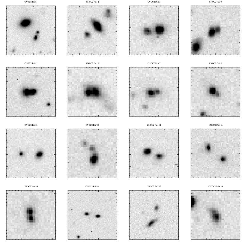
Figure 5: A mosaic of images is given for the 44 close (5 $h^{-1}$ kpc $<r_{p}\leq 20$ $h^{-1}$ kpc) dynamical ($\Delta V<500$ km/s) pairs or triples satisfying the criterion used for computing pair statistics. These $R_{C}-$band images were obtained using the CFHT MOS. Each image is 50 $h^{-1}$ kpc  on a side, corresponding to typical angular sizes of $\sim$ 20″. For images which contain more than two objects, note that (a) the image is centered on the pair, (b) the faintest galaxies may fall below the flux limit, and (c) other objects may be stars or foreground/background galaxies.

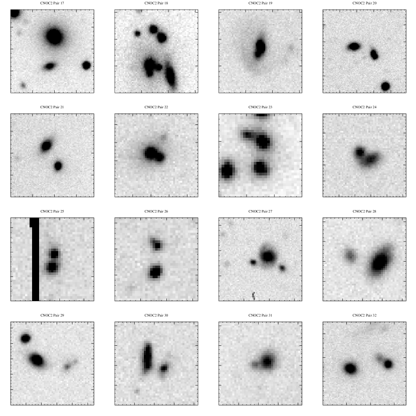
Figure 5: Continued

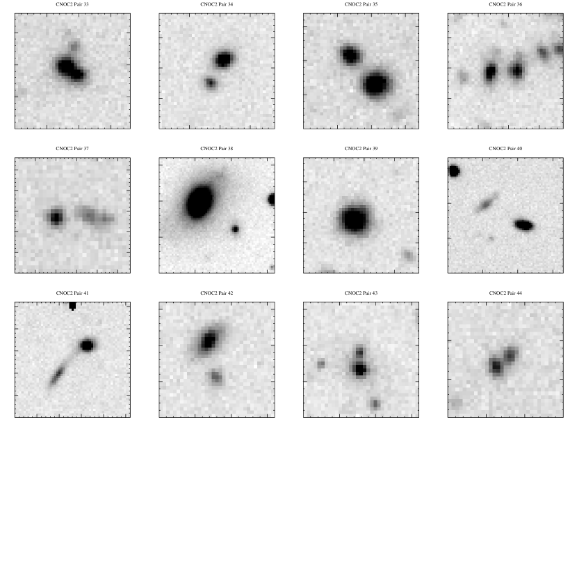
Figure 5: Continued

We have now set out an approach for measuring pair statistics for the CNOC2 survey. We define a close companion to be one with a projected physical separation of 5 $h^{-1}$ kpc $\leq r_{p}\leq$ 20 $h^{-1}$ kpc  and a rest-frame line-of-sight velocity difference of $\Delta v\leq$ 500 km/s. Using this definition, and the survey parameters set out above, we find a total of 88 close companions in CNOC2. When using the same range in absolute magnitude for the primary and secondary samples ($-21\leq M_{B}^{k,e}\leq-18$) as we have done here, a given galaxy pair usually contributes two companions. For CNOC2, this is the case for all of our pairs; furthermore, no spectroscopic triples are found. Thus, our 88 close companions are found in 44 unique pairs. In Tables 1$-$4, we present the following properties of these pairs: Pair ID, CNOC2 ID (PPP number) for each galaxy, projected physical separation ($r_{p}$) and rest-frame line-of-sight velocity difference ($\Delta v$) of the galaxies, coordinates of the pair center, and the mean redshift of the pair. A histogram of companion absolute magnitudes is given in Figure 4. We also present a mosaic of $R_{C}$ images for these systems in Figure 5. Some of these pairs exhibit clear signs of interactions; however, in most cases, the poor resolution of these ground based images renders classification uncertain at best. Hubble Space Telescope imaging of these pairs will be presented in a forthcoming paper (D.R. Patton, in preparation).

Using this sample of companions, pair statistics were computed for each of the 4 CNOC2 patches. Errors were computed using the Jackknife technique. These results are given in Table 5, along with the number of galaxies used in each sample (N) and the observed number of companions (${\rm N}_{{\rm comp}}$). Results from the 4 patches were combined, weighting by Jackknife errors, to give $N_{c}=0.0321\pm 0.0077$ and $L_{c}=0.0294\pm 0.0084\times 10^{10}~{}h^{2}L_{\odot}$ at $z$=0.30. Results from all 4 patches are consistent with these mean values, within the quoted 1$\sigma$ errors. We now investigate how sensitive these results are to the particular parameters selected in this study.

6.1 Dependence on Limiting Absolute Magnitude

We have stressed the importance of specifying a range in absolute magnitude for companions, when computing pair statistics. The faint limit (hereafter $M_{2}$) is particularly important. For this study, we have selected $M_{2}(B)$=$-18$ as being representative of our sample (see § 4.5). It is useful to see how our results change with different choices of this important parameter. We now compute our pair statistics for $-19\leq M_{2}\leq-17$. The results, after combining all 4 patches, are given in Table 7.

Both $N_{c}$ and $L_{c}$ are expected to increase as $M_{2}$ becomes fainter, and this is seen in Table 7. $N_{c}$ increases by a factor of $\sim 5$ between $M_{2}$=$-19$ and $M_{2}$=$-17$. $L_{c}$ is less sensitive to $M_{2}$, changing by a factor of $\sim 2$ over the same range. In both cases, the changes are due solely to the increase in mean number or luminosity density, resulting from integrating deeper into the LF. These trends are very similar to what P2000 found for SSRS2, and further emphasize the importance of accounting for sample depth when computing pair statistics.

6.2 Dependence on $r_{p}^{\rm{max}}$

Close companions are required to have projected separations less than $r_{p}^{\rm{max}}=20$ $h^{-1}$ kpc. While this maximum separation is thought to be ideal for isolating good merger candidates, it is useful to see how the pair statistics behave at larger separations. With this in mind, we compute pair statistics for 10 $h^{-1}$ kpc$\leq r_{p}^{\rm{max}}\leq 100~{}$$h^{-1}$ kpc, with $\Delta v^{\rm{max}}=500$ km/s. Results are given in Figure 6. This plot indicates a smooth increase in both $N_{c}$ and $L_{c}$ with $r_{p}^{\rm{max}}$. This trend is expected from measurements of the galaxy correlation function. This function is commonly expressed as a power law of the form $\xi(r,z)=(r_{0}/r)^{\gamma}$, with $\gamma$=1.8 (Davis & Peebles, 1983). Integration over this function yields pair statistics that vary as $r_{p}^{3-\gamma}\approx r_{p}^{1.2}$, which is in good agreement with the trend found in Figure 6.

6.3 Dependence on $\Delta v^{\rm{max}}$

We also compute pair statistics for a range in $\Delta v^{\rm{max}}$. This is done first for $r_{p}^{\rm{max}}=20$ $h^{-1}$ kpc, showing the relative contributions at different velocities to the mean pair statistics quoted in this study. We also compute statistics using $r_{p}^{\rm{max}}=50~{}$$h^{-1}$ kpc, in order to improve the statistics. Results are given in Figure 7. Two important conclusions may be drawn from this plot. First, at small velocities, both $N_{c}$ and $L_{c}$ increase with $\Delta v^{\rm{max}}$, as expected. This simply indicates that one continues to find additional companions as the velocity threshold increases. Secondly, the pair statistics begin to flatten out at around $\Delta v^{\rm{max}}$=500 km/s. Increasing the threshold to 1000 km/s or higher does increase the size of the pair sample substantially. Moreover, the additional pairs that would be found would be less likely (on average) to be good merger candidates. We conclude that $\Delta v^{\rm{max}}=500$ km/s is a sensible and efficient choice. The main results of this study are unaffected by small changes in the choice of $\Delta v^{\rm{max}}$.

7 MERGER RATE EVOLUTION

Having computed pair statistics at moderate redshift, we now compare our measurements with the results of P2000 to infer evolution in the galaxy merger and accretion rates from $z\sim 0.3$ to $z\sim 0$. We begin by justifying a direct comparison of these two samples. After estimating the evolution in the merger and accretion rates, we will explore the sensitivity of our results to various assumptions that have been made in this analysis.

7.1 Validity of Comparison

Throughout this study, we have stressed the importance of making careful measurements of pair statistics, to avoid various biases that may adversely affect the results. Here, we review the important issues that must be addressed before comparing pair statistics for different samples.

First of all, one must ensure that the definition of a close companion is identical in all samples. When comparing samples at different redshifts, one must be cautious of definitions that may have redshift-dependent biases present. For example, earlier photometric studies of galaxy pairs (e.g., Zepf & Koo 1989) had to correct for optical contamination due to unrelated foreground or background galaxies. While this contamination can be accounted for, the degree of contamination increases systematically with redshift; hence, it is clearly preferable to avoid this correction, by using companions with measured redshifts. For both SSRS2 and CNOC2, we have used the same definition of a close companion. Our dynamical definition is unaffected by optical contamination, or other redshift-dependent biases. The only remaining factor that may cause our definition to change with redshift is the choice of cosmology. That is, if our choice of cosmological parameters is not correct, there will be a redshift-dependent change in the projected physical separation used to identify close companions. In Section 7.5, we explore the effects that different choices of cosmological parameters have on our estimates of merger rate evolution.

There are two passband effects that must be considered when comparing different samples. First, any limits in absolute magnitude must be the same for all samples. For both SSRS2 and CNOC2, we compute pair statistics in rest-frame $B$. It is also important to select galaxies at approximately the same rest-frame wavelength. If this is not done, any differences in the resulting pair statistics may simply be artifacts of the selection process. The SSRS2 sample was selected in $B$. The CNOC2 sample was selected in observed $R_{C}$, which is roughly equivalent to rest-frame $B$ at $z\sim 0.4$. Thus, SSRS2 and CNOC2 are selected at comparable rest-frame wavelengths.

Finally, we have emphasized the need to specify a range in absolute magnitude for computing pair statistics. When comparing different samples, it is critical that this correspond to the same intrinsic luminosity in all samples. P2000 computed pair statistics for SSRS2 using $-21\leq M_{B}\leq-18$. For CNOC2, we have chosen the same range in absolute magnitude, accounting for $k$-corrections and luminosity evolution. This helps to ensure that we are probing the same range in galaxy masses at all redshifts.

7.2 Merger Rate Evolution Using $r_{p}^{\rm{max}}$ = 20 $h^{-1}$ kpc

Having demonstrated that it is reasonable to compare our SSRS2 and CNOC2 pair statistics, we now proceed with the analysis. P2000 computed pair statistics for the SSRS2 survey (da Costa et al., 1998), which consists of 5426 galaxies at $z\sim 0$. Primary and secondary samples were drawn from the same set of galaxies. Using close (5 $h^{-1}$ kpc  $\leq r_{p}\leq$ 20 $h^{-1}$ kpc) dynamical ($\Delta v\leq 500$ km/s) pairs, the resulting pair statistics were as follows : $N_{c}(-21\leq M_{B}^{k,e}\leq-18)=0.0226\pm 0.0052$ and $L_{c}(-21\leq M_{B}^{k,e}\leq-18)=0.0216\pm 0.0055\times 10^{10}~{}h^{2}L_{\odot}$ at $<$$z$$>$=0.015.

CNOC2 pair statistics were given in Table 5. Pair statistics for both SSRS2 and CNOC2 are plotted in the lower portion of Figure 8. Recall that $N_{c}$ is related to the galaxy merger rate, while $L_{c}$ depends on the mass accretion rate. Following the convention in this field, we choose to parameterize evolution in the galaxy merger rate by $(1+z)^{m_{N}}$, where $m_{N}$ is determined by changes in $N_{c}$ with redshift. Similarly, we take the accretion rate to evolve as $(1+z)^{m_{L}}$. We find $m_{N}=1.44\pm 1.34$ and $m_{L}=1.34\pm 1.55$. These relations are plotted in Figure 8.

7.3 Merger Rate Evolution Using $r_{p}^{\rm{max}}$ = 50 $h^{-1}$ kpc

The preceding results provide some support for a mild rise in the merger and accretion rates with redshift. However, the error bars are uncomfortably large. There simply are not enough small separation pairs in our sample to give a definitive answer. It is possible to improve on this result by relaxing our definition of a close pair. In particular, Figure 6 indicates that both $N_{c}$ and $L_{c}$ vary smoothly with $r_{p}^{\rm{max}}$. In order to get a better handle on the evolution in the merger and accretion rates, we therefore choose to increase $r_{p}^{\rm{max}}$ to 50 $h^{-1}$ kpc. Pair statistics were computed for both CNOC2 and SSRS2, and are given in Table 6 (see also Figure 8). These estimates yield merger and accretion rates which evolve as $m_{N}=2.26\pm 0.70$ and $m_{L}=2.28\pm 0.89$. We will take these to be our most secure estimates of evolution in the merger and accretion rates.

7.4 Dependence on Modelling of Luminosity Evolution

In Section 4.2, we outlined our approach for modelling luminosity evolution in our sample, using the $Q$ parameter derived from measurements of the CNOC2 LF (Lin et al., 1999). When computing pair statistics, we have taken $Q$=1, which assumes an average of $z$ magnitudes of luminosity evolution at redshift $z$. To see how this assumption affects our results, we recompute the pair statistics (with $r_{p}^{\rm{max}}$=50 $h^{-1}$ kpc) using different choices of $Q$. For $Q$=0 (no evolution) we find $m_{N}=3.07\pm 0.72$ and $m_{L}=3.85\pm 0.85$. Thus, if we do not account for luminosity evolution, we infer a stronger increase in the merger and accretion rates with redshift. For $Q$=2, we find $m_{N}=1.40\pm 0.67$ and $m_{L}=0.70\pm 0.94$. In both cases, the effects are strongest for $L_{c}$, which has an additional luminosity, and hence Q, dependence. The size of these effects demonstrates the importance of compensating for luminosity evolution when computing pair statistics. Nevertheless, for physically plausible choices of $Q$, our estimates of $m_{N}$ and $m_{L}$ are not dominated by uncertainty in the amount of luminosity evolution that is present.

7.5 Dependence on Cosmology

The choice of cosmological parameters affects the computed value of $r_{p}$ for each pair, and also changes the inferred luminosity of all galaxies in the sample. It is therefore important to determine the dependence of $m_{N}$ and $m_{L}$ on these parameters. At $z$=0.3, $r_{p}$ is $\sim 6\%$ smaller for $q_{0}$=0.5 than for our choice of $q_{0}$=0.1. Therefore, for a fixed maximum projected separation ($r_{p}^{\rm{max}}$), this increases the angular search area, and thereby the number of close companions. However, this effect is countered by the decreased luminosities that result from reduced luminosity distances (see eq. 2). Decreasing galaxy luminosities lowers the number and luminosity density of galaxies in the range of interest here ($-21\leq M_{B}^{k,e}\leq-18$). The choice of $q_{0}$ also affects measurement of the galaxy LF, which is needed for measuring pair statistics for this flux-limited sample. Lin et al. (1999) have measured the CNOC2 LF for both $q_{0}$=0.1 and $q_{0}$=0.5. The SSRS2 and CNOC2 pair statistics were recomputed using $q_{0}$=0.5 and $r_{p}^{\rm{max}}$=50 $h^{-1}$ kpc. We find $m_{N}=2.13\pm 0.67$ and $m_{L}=1.91\pm 0.88$. That is, while a small reduction is seen in the evolution of $N_{c}$ and $L_{c}$, the competing effects of decreased $r_{p}$ and decreased luminosities nearly cancel out.

The pair statistics may also change in the presence of a non-zero cosmological constant. Using values of $\Omega_{M}$=0.2 and $\Omega_{\Lambda}$=$0.8$, $r_{p}$ increases by about $\sim 6\%$ at $z$=0.3. This effect is comparable in size but opposite in direction to the example given in the preceding paragraph. This implies that this non-zero $\Lambda$ cosmology would causes a small increase in the amount of evolution in the merger and accretion rates. We conclude that our pair statistics are insensitive to the choice of $q_{0}$ and $\Omega_{\Lambda}$. The choice of cosmological parameters will become more of an issue as studies of galaxy pairs are extended to higher redshifts (e.g., Carlberg et al. 2000a).

8 DISCUSSION

8.1 Summary of New Results

We have used the CNOC2 redshift survey to compute secure measurements of close pair statistics at $z\sim 0.30$. These are the first measurements at $z>0$ that use only dynamically confirmed pairs ($\Delta v<500$ km/s). Moreover, we have carefully accounted for a number of selection biases that may have adversely affected earlier estimates. In particular, we have accounted for the dependence on the limiting absolute magnitude of companions; without this crucial step, it is very dangerous to compare pair statistics from different surveys. This is also the first study to include an explicit correction for the redshift-dependent bias introduced by luminosity evolution.

Following the techniques outlined by P2000, we have computed pair statistics using the number and luminosity of companions. $N_{c}$ gives the number of close companions per galaxy, while $L_{c}$ measures the luminosity in close companions, per galaxy. We find $N_{c}(-21\leq M_{B}^{k,e}\leq-18)=0.0321\pm 0.0077$ and $L_{c}(-21\leq M_{B}^{k,e}\leq-18)=0.0294\pm 0.0084\times 10^{10}~{}h^{2}L_{\odot}$ at $z$=0.30. After increasing the maximum pair separation to 50 $h^{-1}$ kpc, and comparing with the low redshift SSRS2 pairs sample, we infer evolution in the galaxy merger and accretion rates of about $(1+z)^{2.3\pm 0.7}$ and $(1+z)^{2.3\pm 0.9}$ respectively.

8.2 Comparison With Earlier Studies

As with earlier close pair studies, we have arrived at an estimate of the degree of evolution in the galaxy merger rate. These studies have yielded a wide variety of results in the past (see Patton et al. 1997 for a review). Using a consistent transformation between the pair fraction and merger rate, results parameterized by $(1+z)^{m}$ vary from $m\sim 0$ (Woods, Fahlman, & Richer, 1995) to $m\sim 5$ (Zepf & Koo, 1989; Yee & Ellingson, 1995). After accounting for various discrepancies due to optical contamination and spectroscopic completeness, these results were shown to be roughly consistent with the value of $m=2.8\pm 0.9$ derived by Patton et al. (1997). More recently, Le Fèvre et al. (2000) estimated the merger rate to evolve as $m=2.7\pm 0.6$, using Hubble Space Telescope imaging of the CFRS and LDSS redshift surveys.

Despite the apparent convergence in results, one must be very careful when comparing samples of close pairs at different redshifts. If differences exist in the limiting absolute magnitudes of the samples, or if there are systematic differences in the way galaxies and pairs are selected, any resulting merger rate estimate may be strongly affected by redshift-dependent selection effects (P2000). In our judgement, this paper provides the first published estimate of merger rate evolution that satisfies these important criteria.

It is worth noting that, despite an order of magnitude increase in redshift survey sizes, the uncertainties in our merger rate estimates are still comparable in size to those of Patton et al. (1997) and Le Fèvre et al. (2000). There are several reasons for this. The primary difference in our pair sample is that we have required all pairs to have redshifts for both members. This yields results that are on a much more secure footing than earlier studies which incorporated the use of companions with and without redshifts. We have purified our pair sample further by requiring $\Delta v\leq 500$ km/s. We have also restricted our sample in redshift and luminosity, in order to minimize the detrimental effects of luminosity-dependent clustering. All of these effects have made our sample more secure, but have greatly reduced the size of our sample. Finally, we have computed uncertainties using the Jackknife technique, which is well-suited to the weighted pair statistics used in this study. These error estimates were found to be larger than Poisson statistics, by a factor of $\approx\sqrt{2}$. The reason for this difference lies in a subtle but important detail regarding the application of Poisson statistics to pairs. The number of independent objects being counted is the number of pairs, rather than the number of galaxies in pairs. In Patton et al. (1997), as in earlier studies, this was not recognized, leading to uncertainties that were underestimated by a factor of $\sqrt{2}$.

8.3 Implications

In order to interpret our merger rate estimates, it is useful to consider several simple scenarios. First, for a universe with fixed co-moving density and no clustering, the physical density increases as $(1+z)^{3}$. As our pair statistics measure the number and luminosity of companions within a fixed physical volume (determined by $r_{p}^{\rm{max}}$ and $\Delta v^{\rm{max}}$), they would be expected to increase at the same rate. Of course, there is likely to be evolution in the co-moving number density of galaxies, as indicated from studies of the galaxy LF. These changes will translate, on average, into comparable changes in pair statistics. We must also consider the effects of clustering on the evolution of the merger rate. The scenario outlined above includes no clustering, and hence is not representative of the real universe. In order to incorporate clustering, we refer to the galaxy correlation function, which provides a convenient parameterization of clustering. This function, and its evolution with redshift, is traditionally parameterized as follows :

$$\xi(r,z)=\xi(r,0)(1+z)^{-(3+\epsilon)},$$ (19)

where

$$\xi(r,0)=\left({r\over r_{0}}\right)^{-\gamma}.$$ (20)

Our pair statistics are proportional to the mean physical density, which (in the absence of LF evolution) varies as $(1+z)^{3}$, multiplied by an integral over the correlation function, which varies as $(1+z)^{-(3+\epsilon)}$. Thus, $N_{c}\propto(1+z)^{-\epsilon}$ ($L_{c}$ has the same dependence). Suppose we require that clustering remain fixed in proper (physical) coordinates. This corresponds to $\epsilon$ =0. In this case, the physical density of companions will not evolve. That is, we would expect to find $m_{N}$=$m_{L}$=0. Similarly, we consider a scenario in which the clustering is fixed in co-moving coordinates. In this case, $\epsilon=\gamma-3$. Measurements of the correlation function routinely give $\gamma$ = 1.8 (Davis & Peebles, 1983; Carlberg et al., 2000b). This gives pair statistics that vary as $(1+z)^{1.2}$. Finally, we consider measurements of clustering evolution. Carlberg et al. (2000b) find $\epsilon=-0.17\pm 0.18$, using the CNOC2 survey. These results are measured on scales of roughly 0.1 to 10 $h^{-1}$ Mpc. If we extrapolate their correlation function measurements down to the small scales of interest here, we would expect clustering evolution to cause our pair statistics to vary roughly as $(1+z)^{0.17}$. Our results are inconsistent with this simple clustering evolution scenario at the 3$\sigma$ level.

8.4 The Cumulative Effect of Mergers Since $z\sim$ 1

Following the merger remnant analysis of P2000, we will attempt to interpret the implications of our results for galaxies at the present epoch. We will estimate the fraction of present day galaxies that have undergone mergers in the past, referring to this quantity as the remnant fraction ($f_{{\rm rem}}$). Suppose that a fraction $f_{{\rm mg}}$ of galaxies are undergoing mergers at the present epoch. If we consider a lookback time of $NT_{{\rm mg}}$, where $T_{{\rm mg}}$ is the merger timescale and $N$ is an integer, then

$$f_{{\rm rem}}=1-\prod_{j=1}^{N}{1-f_{{\rm mg}}(z_{j})\over 1-0.5f_{{\rm mg}}(z_{j})},$$ (21)

where $z_{j}$ corresponds to a lookback time of $t=jT_{{\rm mg}}$. We begin by using the estimates of P2000 for the local epoch merger fraction ($f_{{\rm mg}}$=0.011) and the merger timescale ($T_{{\rm mg}}$=0.5 Gyr). We now employ the estimates of merger rate evolution from the present study. We take the merger rate to evolve as $(1+z)^{2.3}$. Using equation 21, with lookback time computed using $h$=0.7 and $q_{0}$=0.5, we find that 15% of $-21\leq M_{B}\leq-18$ galaxies at the present epoch have undergone a major merger since $z\sim 1$. This remnant fraction is roughly twice as large as the no-evolution remnant fraction (P2000). Even so, our result implies that the majority of bright galaxies have not undergone a major merger since $z\sim 1$. We note also that our estimated remnant fraction is similar to the fraction of bright field galaxies that are ellipticals (e.g., Dressler 1980; Postman & Geller 1984). This is consistent with a scenario in which the mergers of bright galaxies produce elliptical galaxies.

8.5 Future Work

It is now clear that only a few percent of bright galaxies are found in close pairs, at least at the modest redshifts under consideration. This makes it challenging to find enough dynamical pairs for statistically useful measurements of pair statistics, even with redshifts surveys of about 5000 galaxies. It is even more difficult for sparsely sampled surveys, since the observed number of pairs scales with the square of the spectroscopic completeness. Further progress may require a relaxation of the requirement that both members of each pair have measured redshifts. We intend to apply our pair statistics to deep imaging of faint galaxies in the vicinity of the CNOC2 galaxies used in this survey. This approach will have the added benefit of extending pair statistics to the regime of minor mergers.

Redshift surveys that probe out to higher redshifts will provide more leverage on evolution in the galaxy merger and accretion rates (e.g., Carlberg et al. 2000a). Our observations - and most models of galaxy formation - indicate that merging is likely to be more prevalent at higher redshifts. However, these samples will be even more susceptible to redshift-dependent selection effects (e.g., $k$-corrections and luminosity evolution); as a result, it will be critical that the pair statistics be corrected for these biases. High redshift surveys used to detect companions based on photometry alone will face the additional challenge of accounting for increased numbers of foreground galaxies,

Finally, any sample of close galaxy pairs can also be used to study the effects of interactions on the galaxies themselves. Of particular importance is the question of enhanced star formation that may result from these close encounters. We have undertaken a number of detailed studies of the CNOC2 galaxy pairs identified in this paper, including high resolution optical imaging with the Hubble Space Telescope (D.R. Patton, in preparation), sub-millimeter continuum observations with the James Clerk Maxwell Telescope, and multi-color imaging and spectroscopy from the CNOC2 survey itself.

Figure 1: $B$ absolute magnitude is plotted versus redshift for all CNOC2 galaxies with $R_{C}\leq 21.5$ and $0.12\leq z\leq 0.55$. The curved line gives the limit imposed by the limiting apparent magnitude, assuming the maximal $k$-correction $k_{R_{C}\rightarrow B}^{\rm{max}}(z)$ at redshift $z$. Note that objects lying below this line are brighter than $R_{C}$=$21.5$ but are blue; Section 4.3 explains why these objects are excluded from the sample. The upper horizontal line indicates the bright limit imposed on the sample($M_{B}^{k,e}$ = $-21$), while the lower horizontal line denotes the faint limit ($M_{B}^{k,e}$ = $-17$). Galaxies satisfying all of these criteria (and hence used in the calculation of $N_{c}$ and $L_{c}$) are marked with triangles; the remainder are indicated with crosses.

Figure 2: Model $k$-corrections from Coleman, Wu, and Weedman (1980) are given for 4 galaxy types. Lines are as follows : E/S0 (long-dashed line), Sbc (dashed line), Scd (dotted line), and Im (solid line). The maximal $k$-correction $k_{R_{C}\rightarrow B}^{\rm{max}}(z)$ is marked with a thick dashed line.

Figure 3: Spectroscopic completeness is computed for a range of angular pair separations. (a) In the upper panel, we compute the ratio of spectroscopic pairs ($N_{\rm zz}$) to photometric pairs ($N_{\rm pp}$), as a function of angular separation $\theta$. Error bars are computed using the Jackknife technique. With fair selection, $N_{\rm zz}/N_{\rm pp}=f_{s}^{2}\approx 0.1753$ (dashed line), as this gives an excellent fit to the completeness on large scales ($\theta>3.5\arcmin$). The incompleteness is modelled with a power law at $10\arcsec<\theta<210\arcsec$. This power law clearly does not provide an acceptable fit on smaller scales; hence, we take $N_{\rm zz}/N_{\rm pp}$=0.129 for $\theta\leq 10\arcsec$. The combined fit is marked with a solid line. (b) The observed spectroscopic completeness is corrected using weights from the modelled fit, and is plotted in the lower panel. The horizontal solid line gives $f_{s}^{2}$=0.1753. The corrected data points are consistent with this value at all separations.

Figure 4: An absolute magnitude histogram is given for the 88 companions used in the pair statistics.

Figure 6: Pair statistics are computed for $\Delta v\leq 500$ km/s, for a range of maximum projected separations ($r_{p}^{\rm{max}}$). A minimum projected separation of $r_{p}=5~{}$$h^{-1}$ kpc is applied in each case. Error bars are computed using the Jackknife technique. Both $N_{c}$ and $L_{c}$ are cumulative statistics; hence, measurements in successive bins are not independent. The line in each panel follows the $r_{p}^{3-\gamma}$ dependence that results from integration over the galaxy two-point correlation function. Taking $\gamma$ = 1.8 and requiring a match with the data at $r_{p}=100~{}$$h^{-1}$ kpc, good agreement is found at all separations.

Figure 7: Pair statistics are computed for a range in $\Delta v^{\rm{max}}$, for both $r_{p}^{\rm{max}}=20~{}$$h^{-1}$ kpc (left panels) and $r_{p}^{\rm{max}}=50~{}$$h^{-1}$ kpc  (right panels). Error bars are computed using the Jackknife technique. Both $N_{c}$ and $L_{c}$ are cumulative statistics; hence, measurements in successive bins are not independent.

Figure 8: Pair statistics ($N_{c}$ and $L_{c}$) are given for SSRS2 ($<$$z$$>$=0.015) and CNOC2 ($<$$z$$>$=0.30). Measurements are given for $r_{p}^{\rm{max}}$=20 $h^{-1}$ kpc (bottom), $r_{p}^{\rm{max}}$=50 $h^{-1}$ kpc (middle), and $r_{p}^{\rm{max}}$=100 $h^{-1}$ kpc (top). Best fit lines indicate evolution varying as $(1+z)^{m}$. For $r_{p}^{\rm{max}}$=(20,50,100) $h^{-1}$ kpc, values of $m$ used are (1.44,2.26,1.66) for $N_{c}$ and (1.34,2.28,1.70) for $L_{c}$. Increases in both $N_{c}$ and $L_{c}$ with redshift are seen for all three choices of $r_{p}^{\rm{max}}$.

Table 1: CNOC2 0223+00 Close Pairs

Pair	CNOC2 ID’s	$r_{p}$	$\Delta v$	RA	DEC	$\bar{z}$
ID	(Galaxy A,B)	($h^{-1}$kpc)	(km/s)	[2000.0]	[2000.0]
1	100810,100778	18.3	103	02:26:53.2	+00:02:44	0.13339
2	140091,140075	13.2	232	02:25:23.0	+00:07:11	0.26693
3	130708,130707	12.7	133	02:25:09.2	+00:18:05	0.35090
4	030307,030309	6.0	162	02:25:49.2	+00:30:30	0.29829
5	191878,191879	6.0	318	02:23:28.3	-00:03:52	0.27009
6	131533,131534	6.7	273	02:25:26.4	+00:21:44	0.40391
7	121099,121101	6.6	63	02:26:17.1	+00:12:47	0.38407
8	041013,041009	5.6	154	02:26:00.5	+00:41:12	0.41931
9	050675,050679	19.1	189	02:25:55.5	+00:47:14	0.27099
10	031099,031118	11.5	264	02:25:49.0	+00:33:57	0.40769
11	140119,140109	12.8	76	02:25:35.4	+00:07:19	0.26747
12	030571,030555	19.4	189	02:25:58.9	+00:31:37	0.30031
13	040997,040989	7.4	62	02:26:17.4	+00:41:12	0.39882
14	160751,160754	11.1	76	02:25:02.5	+00:01:15	0.14997
15	010594,010632	16.6	9	02:26:03.6	+00:17:13	0.26799
16	040345,040350	5.5	101	02:26:13.4	+00:38:22	0.39666

Table 2: CNOC2 0920+37 Close Pairs

Pair	CNOC2 ID’s	$r_{p}$	$\Delta v$	RA	DEC	$\bar{z}$
ID	(Galaxy A,B)	($h^{-1}$kpc)	(km/s)	[2000.0]	[2000.0]
17	010722,010688	18.2	423	09:24:03.2	+37:04:47	0.19171
18	061308,061331	18.1	2	09:24:01.2	+37:44:18	0.24652
19	081315,081301	5.4	284	09:24:39.6	+37:08:16	0.24645
20	050264,050258	13.1	193	09:23:42.8	+37:31:42	0.13640
21	010879,010860	13.8	360	09:24:08.0	+37:05:39	0.19029
22	131238,131230	6.0	50	09:23:12.6	+37:07:05	0.39017
23	172734,172762	16.6	437	09:22:26.9	+36:42:45	0.47497
24	020557,020566	7.4	29	09:23:30.7	+37:11:19	0.32471
25	160826,160832	8.7	198	09:22:27.9	+36:46:52	0.39208
26	191850,191890	17.3	10	09:21:06.9	+36:41:14	0.44085

Table 3: CNOC2 1447+09 Close Pairs

Pair	CNOC2 ID’s	$r_{p}$	$\Delta v$	RA	DEC	$\bar{z}$
ID	(Galaxy A,B)	($h^{-1}$kpc)	(km/s)	[2000.0]	[2000.0]
27	101867,101865	9.6	5	14:50:25.4	+08:56:25	0.14608
28	140046,140054	18.1	404	14:48:56.1	+08:56:44	0.26193
29	162151,162141	18.4	43	14:48:22.0	+08:56:32	0.19365
30	120368,120356	12.1	212	14:49:45.8	+08:57:30	0.27244
31	110843,110838	6.5	172	14:49:27.0	+08:52:10	0.26965
32	011270,011283	19.5	94	14:49:33.1	+09:10:53	0.21406
33	051065,051056	5.9	138	14:49:55.1	+09:38:43	0.34926
34	161997,161985	12.0	111	14:48:12.9	+08:55:53	0.32429
35	082155,082172	16.2	171	14:50:05.9	+09:11:54	0.36420
36	091998,091999	11.7	41	14:50:09.9	+09:04:35	0.32469
37	040704,040709	15.0	44	14:49:38.9	+09:29:30	0.51024

Table 4: CNOC2 2148-05 Close Pairs

Pair	CNOC2 ID’s	$r_{p}$	$\Delta v$	RA	DEC	$\bar{z}$
ID	(Galaxy A,B)	($h^{-1}$kpc)	(km/s)	[2000.0]	[2000.0]
38	070479,070450	19.8	249	21:51:11.5	-04:47:59	0.15447
39	180896,180907	6.6	107	21:49:18.5	-05:58:46	0.31239
40	141675,141692	18.4	115	21:50:56.9	-05:38:54	0.14462
41	031553,031529	16.9	48	21:51:12.7	-05:17:46	0.19767
42	071349,071332	16.8	143	21:51:22.0	-04:45:16	0.40839
43	131817,131825	7.9	6	21:50:36.8	-05:29:30	0.42589
44	162261,162264	8.1	125	21:50:16.5	-05:45:46	0.50631

Table 5: CNOC2 Pair Statistics

Sample	N	Ncomp	$\bar{z}$	$N_{c}$	$L_{c}(10^{10}h^{2}L_{\odot})$
0223	1150	32	0.309	0.0538$\pm$ 0.0205	0.0451$\pm$ 0.0215
0920	1094	20	0.301	0.0252$\pm$ 0.0113	0.0268$\pm$ 0.0134
1447	961	22	0.301	0.0363$\pm$ 0.0166	0.0311$\pm$ 0.0173
2148	979	14	0.277	0.0280$\pm$ 0.0176	0.0213$\pm$ 0.0180
CNOC2	4184	88	0.297	0.0321$\pm$ 0.0077	0.0294$\pm$ 0.0084

Table 6: Pair Statistics Using $r_{p}^{\rm{max}}$ = 50 $h^{-1}$ kpc

Sample	N	Ncomp	$\bar{z}$	$N_{c}$	$L_{c}(10^{10}h^{2}L_{\odot})$
SSRS2	4769	276	0.015	0.0788$\pm$ 0.0099	0.0613$\pm$ 0.0095
CNOC2	4184	389	0.298	0.1371$\pm$ 0.0163	0.1072$\pm$ 0.0166

Table 7: CNOC2 Pair Statistics for Various Choices of $M_{2}(B)$

$M_{2}$	$N_{c}$	$L_{c}(10^{10}h^{2}L_{\odot})$
-19.0	0.0120$\pm$ 0.0029	0.0184$\pm$ 0.0052
-18.9	0.0137$\pm$ 0.0033	0.0197$\pm$ 0.0056
-18.8	0.0154$\pm$ 0.0037	0.0210$\pm$ 0.0060
-18.7	0.0172$\pm$ 0.0041	0.0223$\pm$ 0.0064
-18.6	0.0192$\pm$ 0.0046	0.0235$\pm$ 0.0067
-18.5	0.0211$\pm$ 0.0050	0.0246$\pm$ 0.0070
-18.4	0.0232$\pm$ 0.0055	0.0257$\pm$ 0.0073
-18.3	0.0253$\pm$ 0.0060	0.0267$\pm$ 0.0076
-18.2	0.0275$\pm$ 0.0066	0.0277$\pm$ 0.0079
-18.1	0.0298$\pm$ 0.0071	0.0286$\pm$ 0.0082
-18.0	0.0321$\pm$ 0.0077	0.0294$\pm$ 0.0084
-17.9	0.0345$\pm$ 0.0082	0.0302$\pm$ 0.0086
-17.8	0.0369$\pm$ 0.0088	0.0310$\pm$ 0.0088
-17.7	0.0394$\pm$ 0.0094	0.0317$\pm$ 0.0090
-17.6	0.0419$\pm$ 0.0100	0.0323$\pm$ 0.0092
-17.5	0.0445$\pm$ 0.0106	0.0329$\pm$ 0.0094
-17.4	0.0471$\pm$ 0.0112	0.0334$\pm$ 0.0096
-17.3	0.0498$\pm$ 0.0119	0.0340$\pm$ 0.0097
-17.2	0.0525$\pm$ 0.0125	0.0344$\pm$ 0.0098
-17.1	0.0553$\pm$ 0.0132	0.0349$\pm$ 0.0100
-17.0	0.0581$\pm$ 0.0139	0.0353$\pm$ 0.0101

References

- Barnes (1988) Barnes, J. E. 1988, ApJ, 331, 699
- Burkey et al. (1994) Burkey, J. M., Keel, W. C., Windhorst, R. A., & Franklin, B. E. 1994, ApJ, 429, L13
- Carlberg, Pritchet, & Infante (1994) Carlberg, R. G., Pritchet, C. J., & Infante, L. 1994, ApJ, 435, 540
- Carlberg et al. (2000a) Carlberg, R. G., et al. 2000a, ApJ, 532, L1
- Carlberg et al. (2000b) Carlberg, R. G., Yee, H. K. C., Morris, S. L., Lin, H., Hall, P., Patton, D. R., Sawicki, M., & Shepherd, C. W. 2000b, ApJ, 542, 57
- Coleman, Wu, and Weedman (1980) Coleman, G. D., Wu, C., & Weedman, D. W. 1980, ApJ, 43, 393
- da Costa et al. (1998) da Costa, L. N., et al. 1998, AJ, 116, 1
- Davis & Peebles (1983) Davis, M., & Peebles, P. J. E. 1983, ApJ, 267, 465
- Dressler (1980) Dressler, A. 1980, ApJ, 236, 351
- Ellis (1997) Ellis, R. S. 1997, ARA&A, 35, 389
- Fukugita et al. (1995) Fukugita, M., Shimasaku, K., & Ichikawa, T. 1995, PASP, 107, 945
- Le Fèvre et al. (2000) Le Fèvre, O., et al. 2000, MNRAS, 311, 565
- Lin et al. (1999) Lin, H., Yee, H. K. C., Carlberg, R. G., Morris, S. L., Sawicki, M., Patton, D. R., Wirth, G., & Shepherd, C. W. 1999, ApJ, 518, 533
- Patton et al. (1997) Patton, D. R., Pritchet, C. J., Yee, H. K. C., Ellingson, E., & Carlberg, R. G. 1997, ApJ, 475, 29
- Patton et al. (2000) Patton, D. R., Carlberg, R. G., Marzke, R. O., Pritchet, C. J., da Costa, L. N. & Pellegrini, P. S. 2000, ApJ, 536, 153 (P2000)
- Postman & Geller (1984) Postman, M., & Geller, M. J. 1984, ApJ, 281, 95
- Sanders & Mirabel (1996) Sanders, D. B., & Mirabel, I. F. 1996, ARA&A, 34, 749
- Schechter (1976) Schechter, P. 1976, ApJ, 203, 297
- Struck (1999) Struck, C. 1999, Phys. Rep., 321, 1
- Woods, Fahlman, & Richer (1995) Woods, D., Fahlman, G. G., & Richer, H. B. 1995, ApJ, 454, 32
- Yee (1991) Yee, H. K. C. 1991, PASP, 103, 396
- Yee & Ellingson (1995) Yee, H. K. C., & Ellingson, E. 1995, ApJ, 445, 37
- Yee, Ellingson, & Carlberg (1996) Yee, H. K. C., Ellingson, E., & Carlberg, R. G. 1996, ApJS, 102, 269
- Yee et al. (2000) Yee, H. K. C., et al. 2000, ApJS, 129, 475
- Zepf & Koo (1989) Zepf, S. E., & Koo, D. C. 1989, ApJ, 337, 34