Chemical abundances in an UV–selected sample of galaxies

Abstract

We discuss the chemical properties of a sample of UV-selected intermediate-redshift ($0\la z\la 0.4$) galaxies in the context of their physical nature and star formation history. This work represents an extension of our previous studies of the rest-frame UV luminosity function (Treyer et al. 1998) and the star formation properties of the same sample (Sullivan et al. 2000, 2001). We revisit the optical spectra of these galaxies and perform further emission-line measurements restricting the analysis to those spectra with the full set of emission lines required to derive chemical abundances. Our final sample consists of 68 galaxies with heavy element abundance ratios and both UV and CCD $B$-band photometry. Diagnostics based on emission-line ratios show that all but one of the galaxies in our sample are powered by hot, young stars rather than by an AGN. Oxygen-to-hydrogen (O/H) and nitrogen-to-oxygen (N/O) abundance ratios are compared to those of various local and intermediate-redshift samples. Our UV-selected galaxies span a wide range of oxygen abundances, from $\sim$ 0.1 to 1 Z_⊙, intermediate between low-mass Hii galaxies and massive starburst nuclei. For a given oxygen abundance, most have strikingly low N/O values. Moreover, UV-selected and Hii galaxies systematically deviate from the usual metallicity-luminosity relation in the sense of being more luminous by 2-3 magnitudes. Adopting the “delayed-release” chemical evolution model, we propose our UV-selected sources are observed at a special stage in their evolution, following a powerful starburst which enriched their ISM in oxygen and temporarily lowered their mass-to-light ratios. We discuss briefly the implications of our conclusions on the nature of similarly-selected high-redshift galaxies.

1 Introduction

Considerable progress has been made recently in understanding the history of galaxy formation and evolution, following the analyses of deep surveys, such as the Hubble Deep Field (Williams et al. 1996), the Canada-France Redshift Survey (Lilly et al. 1995) and the population of Lyman-break galaxies (LBGs) (Steidel et al. 1996, 1999). A popular viewpoint is one that postulates that the bulk of cosmic star formation occurred at redshifts between $\sim$ 1 and 2 (e.g., Madau, Pozetti & Dickinson 1998), in which case the higher redshift LBG population represents an early phase of galaxy formation.

However, the physical nature of the high redshift star-forming galaxies remains unclear, and this hinders our understanding of how they connect with present-day massive galaxies. In particular, it remains unclear to what extent the detectable (i.e. bright and star-forming) high-$z$ galaxies are representative of the entire galaxy population that exists in the distant universe. The large number of starburst-like objects detected questions the classical “standard” scenarios for the evolution of Hubble sequence galaxies, which involve slowly decreasing, regular star formation histories.

Characterizing the recurrence of starbursts in galaxies is one way of addressing the above issues. Do galaxies experience only one or two major bursts of star formation during their life, or is the starburst phenomenon a repetitive one that could mimic continuous star formation on cosmological time-scales?

This question has been addressed recently by Kauffmann, Charlot & Balogh (2001), who explored numerical models of galaxy evolution in which star formation occurs in two modes: a low-efficiency continuous mode, and a high-efficiency mode triggered by interactions with a satellite. With these assumptions, the star formation history of low-mass galaxies is characterized by intermittent bursts of star formation separated by quiescent periods lasting several Gyrs, whereas massive galaxies are perturbed on time-scales of several hundred Myrs and thus have fluctuating but relatively continuous star formation histories. In these models, merger rates are specified using the predictions of hierarchical galaxy formation models (e.g. Kauffmann & Charlot 1998; Cole et al. 2000; Somerville, Primack & Faber 2001).

Examining the chemical evolution and physical nature of star-forming galaxies over a range of redshifts will shed light on this issue. Emission lines from Hii regions have long been the primary means of chemical diagnosis in local galaxies, but this method has only recently been applied to galaxies at cosmological distances following the advent of infrared spectrographs on 8 to 10-m class telescopes (e.g. Steidel et al. 1996; Kobulnicky & Zaritsky 1999; Kobulnicky & Koo 2000; Carollo & Lilly 2001; Hammer et al. 2001; Pettini et al. 1998, 2001) .

The aim of this paper is to derive the chemical properties of a local to intermediate-redshift ($0\la z\la 0.4$) UV-selected sample of galaxies as a further probe of their physical nature and star formation history. A key finding from earlier papers in this series is the possibility that the star formation in a large fraction of these objects is intermittent, contributing significantly to the local UV luminosity density (Sullivan et al. 2000, 2001). The manner in which this links to the chemical history may, when used similarly with high redshift sources, give insight into the nature and evolution of star-forming galaxies over a range of redshift.

Work on the nature of distant and young galaxies, like the LBGs, greatly benefits from studies of their analogues in the nearby universe. Early works revealed evidence that LBGs resemble local UV-bright starburst galaxies in many respects (e.g. Heckman et al. 1998; Meurer, Heckman & Calzetti 1999; Papovich, Dickinson & Ferguson 2001). Although physically larger and more luminous, they share similar star formation rates (SFR) per unit area (Meurer et al. 1997), similar rest-frame UV-to-optical spectral energy distributions (Conti, Leitherer & Vacca 1996; Lowenthal et al. 1997; Pettini et al. 1998, 2001; Papovich, Dickinson & Ferguson 2001), as well as similar interstellar medium dynamical states (Franx et al. 1997; Kunth et al. 1998; Pettini et al. 1998, 2001).

A plan of the paper follows. In Section 2 we give a brief summary of the overall properties of our original UV-selected sample of galaxies. In Section 3 we present new measurements of emission lines and define a subsample of 68 UV-selected galaxies for which heavy element abundance measurements are possible. The locus of the UV-selected galaxies in standard diagnostic diagrams is investigated (Sect. 3.2) to determine their main source of ionization. We search for the spectral signatures of Wolf-Rayet stars (Sect. 3.3). Empirical methods, based on strong emission-line ratios, are presented in Section 4 to derive the O/H and N/O abundance ratios of the sample galaxies. In Section 5 we study how our sample compares with two fundamental scaling relations: N/O versus O/H, and the metallicity-luminosity relation. We summarize our principal conclusions in Section 6. Throughout this paper, all calculations assume an $\Omega=1$ and $\rm H_{0}=100$ km s^-1 Mpc^-1 cosmology.

2 The parent UV-selected galaxy sample

A detailed description of the parent sample from which the analyses in this paper are based can be found in Sullivan et al. (2000, hereafter S2000). Briefly, the fields were first imaged in the UV using the balloon-borne FOCA telescope, a 40cm Cassegrain mounted on a stratospheric gondola, stabilised to within a radius of 2″ rms (see Milliard et al. 1992 for a full description of the experiment). The spectral response of the UV filter approximates a Gaussian centred at 2015 Å, FWHM 188 Å. The camera was operated in two modes – FOCA 1000 (f/2.56, 2.3°) and FOCA 1500 (f/3.85, 1.55°) – with a large field-of-view well suited to survey work. The limiting depth of the exposures we used is $m_{\rm UV}$ $=18.5$, which, for a late-type galaxy, corresponds to $m_{\rm B}$ $=20-21.5$.

The first field, Selected Area 57 (SA57), is centered on $\mathrm{RA}=13^{\mathrm{h}}03^{\mathrm{m}}53^{\mathrm{s}}$, $\mathrm{Dec.}=+29\degr 20\arcmin 30\arcsec$ (1950) and contains the outer regions of the Coma cluster. The second field is centered on $\mathrm{RA}=11^{\mathrm{h}}42^{\mathrm{m}}46^{\mathrm{s}}$, $\mathrm{Dec.}=+20\degr 10\arcmin 03\arcsec$, and contains the Abell 1367 cluster. Both fields were imaged in both FOCA modes, thus ensuring the most reliable UV photometry. As the astrometric accuracy of FOCA ($\simeq$ 3″ rms for FOCA 1500) is insufficient for generating a spectroscopic target list, the FOCA catalogues were matched with APM scans of the POSS optical plates. When more than one possible optical counterpart was found on the POSS plates within the search radius, the nearest optical counterpart to the UV detection was selected. Around 10% of the UV detections have no obvious counterpart at all on the APM plates, indicating that either some of these detections are spurious, or that the counterpart lies at a fainter $B$ magnitude than the limiting magnitude of the POSS plates ($m_{\rm B}$ $\simeq 21$).

In order to improve the photometric coverage of our survey fields, an extensive, high quality multi-colour survey is currently underway. In this present work, we use new $B$-band CCD photometry obtained with the CFH12K camera on the Canada-France-Hawaii Telescope (CFHT) in place of the APM magnitudes used in previous studies (Treyer et al. 1998; S2000). Further details of this photometry and is relationship to that used earlier will be given in a forthcoming paper (Sullivan et al., in preparation) .

Spectroscopic follow-up of the UV selected sources was conducted on the two FOCA fields using two multi-fiber spectrographs – Hydra on the 3.5-m WIYN telescope ($\lambda\lambda$ 3500–6600 Å), and WYFFOS on the 4.2-m William Herschel Telescope (WHT) ($\lambda\lambda$ 3500–9000 Å) (Treyer et al. 1998, S2000). The latter configuration allows the observation of $\rm H{\alpha}$ emission lines to a redshift of $z\sim 0.4$. Only the flux calibrated data from WYFFOS are used in the present paper. Details of all observing runs and the breakdown of spectroscopic objects can be found in S2000, tables 1 and 2 respectively.

Spectra were analysed using the iraf facility splot and the figaro package gauss. Redshifts were measured by visual inspection, and the equivalent widths (EWs) and fluxes of [O ii] $\lambda$3727, [O iii] $\lambda\lambda$4959,5007, $\rm H{\beta}$ and $\rm H{\alpha}$ determined using both spectral analysis programs. Though the spectral resolution ($\sim$ 10 Å) is good enough to resolve the separate [O iii] $\lambda\lambda$4959,5007 lines, in many cases the $\rm H{\alpha}$ line was blended with the nearby [N ii] $\lambda\lambda$6548,6584 lines, so a deblending routine was run from within splot to allow determination of the fluxes of these individual lines. We did not find any systematic error in the measurement of individual lines which could be due to the deblending procedure. Extinction and stellar absorption corrections were applied using the measured Balmer lines. A full description of these procedures can be found in S2000. Typical examples of galaxy spectra are shown in Treyer et al. (1998, their fig. 1).

3 Emission-line properties

Figure 1: Distributions of a) the $B$-band absolute magnitudes, b) the dereddened $UV-B$ colours, c) the redshifts, and d) the extinction coefficients of the UV-selected galaxy sample with measured chemical abundances. Mean value of the distributions is indicated on top of each panel. The peak at $z\sim 0.02$ in the redshift distribution arises from the Coma and Abell 1367 galaxy clusters.

The analysis of S2000 was essentially concerned with the star formation properties of the UV-selected sample described above, using UV fluxes, Balmer and [O ii] $\lambda$3727 emission lines. Emission-line properties were only briefly discussed with the aim of estimating a possible AGN contamination or metallicity effect in order to explain the extreme ($UV-B$) colours found in $\sim 17$% of the galaxies. Based on [O ii] $\lambda$3727/$\rm H{\beta}$ and [O iii] $\lambda\lambda$4959,5007/$\rm H{\beta}$ line ratios, S2000 found that a fraction of the UV galaxies may indeed qualify as AGNs (their fig. 11). However, the [O ii] $\lambda$3727/$\rm H{\beta}$ diagnostic used in that study is very sensitive to dust extinction corrections, and it is therefore preferable to use the [N ii] $\lambda$6584/$\rm H{\alpha}$ and [S ii] $\lambda\lambda$6717+6731/$\rm H{\alpha}$ line ratios which are much less sensitive to extinction (see sect. 3.2). S2000 also searched for possible extremely metal-poor objects in the UV-selected sample which could account for the extreme ($UV-B$) colours. However oxygen abundances were estimated for only 35 field galaxies in the SA57, and no conclusive results were found.

The goal of this present work is to examine in a more systematic manner the emission-line properties of the UV-selected galaxies. In order to make diagnostic diagrams and estimate chemical abundances for a larger fraction of the sample, we revisit the sample of S2000 and, where an emission line measurement is missing, attempt a new line measurement. We then restrict the S2000 sample to all the galaxy spectra which posses the full set of emission lines (i.e. [O ii] $\lambda$3727, $\rm H{\beta}$, [O iii] $\lambda\lambda$4959,5007, $\rm H{\alpha}$ and [N ii] $\lambda$6584) required to derive chemical abundances. Our final sample consists of 68 galaxies with heavy element abundance ratios, UV and new CCD $B$-band photometry.

3.1 New measurements of emission lines

For consistency with the spectral measurements of S2000, the new emission-line measurements were performed using the splot facility in iraf. In particular, we searched for [S ii] $\lambda\lambda$6717+6731 emission lines in all of the 135 emission-line galaxies in the parent sample, and could make a reliable measurement of these lines in 56 of the objects. Additional measurements of $\rm H{\beta}$ (8 objects), [O iii] $\lambda\lambda$4959,5007 (15 objects), and [N ii] $\lambda$6584 (10 objects) could also be performed. Reddening corrections were applied to the new emission-line fluxes as in S2000. The extinction coefficient $c_{\rm H\beta}$ was estimated from the Balmer decrement $\rm H{\alpha}$/$\rm H{\beta}$, assuming case B recombination with an electron density of 100 cm^-3 and a temperature of $10^{4}$ K (Osterbrock 1989), and using a standard interstellar extinction law (Seaton 1979). As in S2000, $\rm H{\alpha}$ and $\rm H{\beta}$ were also corrected for stellar absorption (prior to computing $c_{\rm H\beta}$).

There are two major sources of uncertainty in the measured emission-line ratios. The first arises from the limited signal/noise ratio of the spectra. These errors are computed directly when using the iraf task splot to derive the emission line parameters. splot provides 1-$\sigma$ errors based on estimates of the noise in the individual spectra. The integration error estimates are derived by error propagation assuming a Poisson statistic model of the pixel sigmas, generated by measuring the noise in the spectra on an individual basis and assuming that the linear continuum has no error (see S2000). Measurement errors were propagated quadratically when deriving emission-line ratios and abundance ratios (cf. Sect. 4).

The second source of error arises from contamination of Balmer emission lines by underlying stellar absorption lines. In most cases, Balmer emission line equivalent widths were directly measured in the galaxy spectra. When this was not possible, a constant value of 2 Å  corresponding to the average measured value, typical for star-forming galaxies (McCall et al. 1985; Olofsson 1995a; González-Delgado, Leitherer & Heckman 1999), was applied. This might be a poor approximation for galaxies with weak $\rm H{\beta}$ emission line. We thus propagated an uncertainty of $\pm 1$ Å on Balmer absorption line equivalent widths in all calculations involving Balmer emission lines. Finally, the error in the derived extinction coefficient $c_{\rm H\beta}$ was included when deriving dereddened emission-line ratios.

Global properties of the sub-sample of 68 UV-selected galaxies are shown in Fig. 1. Dust-corrected UV and $B$-band absolute magnitudes are computed as in S2000 using Calzetti (1997) extinction curve. Note that the dereddened ($UV-B$) colour and $B$-band absolute magnitude distributions differ from those of the original sample (S2000) due to the revised $B$-band photometry. The red tail of the ($UV-B$) colour distribution has been significantly reduced whilst the blue component – which formed an interesting unresolved aspect of the discussion in S2000 – is largely unchanged. The revised optical colours means that a a small fraction of the sample is now assigned a different spectral type and $k$-correction. The effect on the absolute UV luminosities are fairly modest however. The main impact of the revised CCD photometry will be in estimating the spectral energy distributions and consequent $k$-corrections; a topic we will discuss in the forthcoming paper (Sullivan et al., in preparation).

3.2 Nature of the main ionizing source: starburst or AGN?

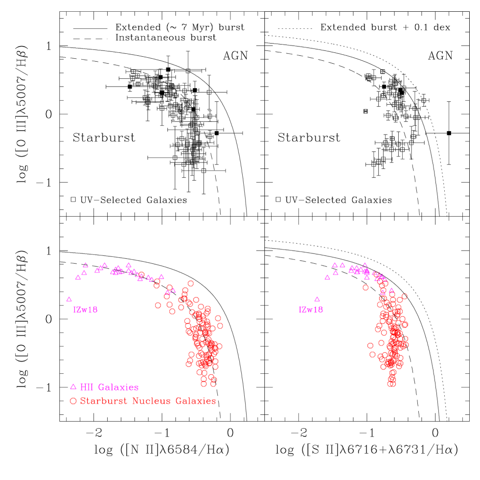
Figure 2: Standard diagnostic diagrams used to classify narrow emission-lines spectra. Top panels. The UV-selected galaxies are shown with their error bars; filled squares are double optical counterpart cases (see text for details). The curves are theoretical boundaries between starburst galaxies and AGNs, assuming an “extended” ($\sim 7$ Myr) burst of star formation (solid line; Kewley et al. 2001) or an “instantaneous” starburst (dashed line; Dopita et al. 2000). The dotted line in the [S ii] $\lambda\lambda$6717+6731/$\rm H{\alpha}$ vs. [O iii] $\lambda$5007/$\rm H{\beta}$ diagram is the upper limit of the starburst model (see text for details). These diagrams show that all the UV-selected galaxies, but one uncertain case which might qualify as a LINER, are powered by hot and young stars rather than by an AGN. Bottom panels. Samples of nearby star-forming galaxies are shown for comparison: Starburst Nucleus Galaxies (circles) selected in the optical (Contini et al. 1998) or in the far-infrared (Veilleux et al. 1995); and Hii galaxies (triangles; see text for references). The location of IZw18, the most metal-poor galaxy known so far, is indicated.

Emission-line diagnostic diagrams can provide a reliable classification of narrow emission-line spectra according to the main source of ionization (hot stars, AGN, or shocks) responsible for these lines. We examine the [O iii] $\lambda$5007/$\rm H{\beta}$ versus [N ii] $\lambda$6584/$\rm H{\alpha}$ and [S ii] $\lambda\lambda$6717+6731/$\rm H{\alpha}$ diagnostic diagrams to discriminate regions photoionized by hot and young stars (i.e. Hii regions) from those photoionized by a harder radiation field, such as that of an AGN or a LINER. Such emission-line ratios are much less sensitive to dust extinction than [O ii] $\lambda$3727/$\rm H{\beta}$, the line ratio previously used in S2000 for this purpose.

The location of the UV-selected galaxies in these diagnostic diagrams is shown in Fig. 2, using dereddened emission-line ratios with their related uncertainties listed in Table 2. In each diagram, the theoretical curves (discussed below) separate star-forming regions (lower left) where the gas is assumed to be ionized by young stars, from AGNs (upper right) where the main ionizing source is thought to be an accretion disk around a black hole. A further distinction among AGN-like objects can be made between high-excitation ([O iii] $\lambda$5007/$\rm H{\beta}$ $>3$) Seyfert 2 galaxies and low-excitation ([O iii] $\lambda$5007/$\rm H{\beta}$ $<3$) LINERs. We did not use the original criteria for defining a LINER (Heckman 1980) because the measurement of [O i] $\lambda$6300 emission lines was generally not possible due to the insufficient S/N of the spectra. For the same reason, we did not use the [O i] $\lambda$6300/$\rm H{\alpha}$ ratio to distinguish between the different sources of ionization.

Two comparative star formation models are shown in Fig. 2: the solid line represents an “extended” burst (i.e. one extending for $\sim 7$ Myr, Kewley et al. 2001) and the dashed line represents an “instantaneous” burst (Dopita et al. 2000). In both cases, the parameters were chosen to span a realistic range of metallicities ($Z=0.1-3.0$ Z_⊙) and ionization parameters ($-3.5\leq\log U\leq-2.0)$. These new theoretical boundaries may provide a more objective classification between Hii regions and the various classes of narrow-line regions associated with AGNs than the classical semi-empirical boundaries defined by Veilleux & Osterbrock (1987).

Clearly, these model predictions have associated uncertainties. These include the assumed chemical abundances and the depletion factors, the slope of the IMF, the stellar evolutionary tracks and the model atmospheres. The dotted line in Fig. 2 (right panel) gives an indication of these uncertainties in the [S ii] $\lambda\lambda$6717+6731/$\rm H{\alpha}$ vs. [O iii] $\lambda$5007/$\rm H{\beta}$ diagram and represents an upper limit to the theoretical boundary between starbursts and AGNs, corresponding to the “extended burst” model $+0.1$ dex (see Kewley et al. 2001 for details).

Figure 2 shows that nearly all the UV galaxies lie below and to the left of the theoretical starburst line. This is especially clear from the [N ii] $\lambda$6584/$\rm H{\alpha}$ vs. [O iii] $\lambda$5007/$\rm H{\beta}$ diagram, where all the galaxies form a well-defined sequence of Hii region-like objects. The distinction is more ambiguous in the [S ii] $\lambda\lambda$6717+6731/$\rm H{\alpha}$ vs. [O iii] $\lambda$5007/$\rm H{\beta}$ diagram. On this plot, a significant fraction of the galaxies are borderline AGN candidates, although they still lie within the error bars of the “extended burst” star formation model.

One galaxy (ID # 24 in Tables 2 and 3) with a relatively high [S ii] $\lambda\lambda$6717+6731/$\rm H{\alpha}$ ratio lies on the right-hand side of the diagram, and could be considered a LINER-type object. However, this galaxy is one of two possible optical counterparts to the UV source. Moreover, the redshifted [S ii] $\lambda\lambda$6717+6731 lines at $z$=0.28 are highly contaminated by bright sky lines, giving a larger uncertainty in this diagnostic than for the bulk of the other sources.

It is instructive to compare the location of the UV-selected galaxies in these diagnostic diagrams with other published samples of nearby star-forming galaxies selected in optical and far-infrared bands. Emission-line ratios for Hii galaxies have been published by Izotov & Thuan (1998) and Izotov, Thuan & Lipovetsky (1994, 1997), and for starburst nucleus galaxies (SBNGs) by Contini et al. (1998) and Veilleux et al. (1995). Both form a well-defined sequence in our two diagnostic diagrams. Hii galaxies are characterized by a high excitation level ([O iii] $\lambda$5007/$\rm H{\beta}$ $\ga 1.5$) and low [N ii] $\lambda$6584/$\rm H{\alpha}$ and [S ii] $\lambda\lambda$6717+6731/$\rm H{\alpha}$ emission-line ratios, whereas SBNGs have lower excitation levels ([O iii] $\lambda$5007/$\rm H{\beta}$ $\la 1$) and higher [N ii] $\lambda$6584/$\rm H{\alpha}$ and [S ii] $\lambda\lambda$6717+6731/$\rm H{\alpha}$ emission-line ratios.

These nearby star-forming galaxies are very well reproduced by the “instantaneous” star formation model in the [N ii] $\lambda$6584/$\rm H{\alpha}$ vs. [O iii] $\lambda$5007/$\rm H{\beta}$ plot, but this is not the case for the [S ii] $\lambda\lambda$6717+6731/$\rm H{\alpha}$ vs. [O iii] $\lambda$5007/$\rm H{\beta}$ diagram. The behavior of SBNGs in this respect is particularly interesting. As the excitation level decreases, the [N ii] $\lambda$6584/$\rm H{\alpha}$ ratio increases whereas the [S ii] $\lambda\lambda$6717+6731/$\rm H{\alpha}$ stay roughly constant. Note also that the star formation models overpredict (by $\sim 0.3$ dex) the [S ii] $\lambda\lambda$6717+6731/$\rm H{\alpha}$ line ratio for SBNGs with the lowest excitation levels.

Figure 2 shows that the major fraction of UV galaxies have excitation levels which are similar to SBNGs whereas extreme Hii galaxies with very low [N ii] $\lambda$6584/$\rm H{\alpha}$ and [S ii] $\lambda\lambda$6717+6731/$\rm H{\alpha}$ ratios are not present in the UV-selected sample. In detail, however, the sequence defined in the [N ii] $\lambda$6584/$\rm H{\alpha}$ vs. [O iii] $\lambda$5007/$\rm H{\beta}$ diagram is somewhat different from the one traced by SBNGs. This is especially true for the low-excitation ([O iii] $\lambda$5007/$\rm H{\beta}$ $\la 1$) UV objects, for which [N ii] $\lambda$6584/$\rm H{\alpha}$ is $\sim 0.1-0.2$ dex lower than for SBNGs. This could be due to chemical enrichment effects. Indeed it has been shown that SBNGs possess a slight overabundance of nitrogen compared to Hii regions with comparable metallicity (Coziol et al. 1999, Considère et al. 2000). This point will be further discussed in section 5.1.

The main conclusion, however, is that the emission-line spectra of all the UV galaxies in our sample, but one dubious case, are powered by hot and young stars rather than by an AGN. We are thus able to derive the chemical properties of the ionized gas in these galaxies using the standard recipes applied for star-forming galaxies.

3.3 Search for Wolf-Rayet stars

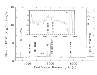
Figure 3: Restframe optical spectrum of an UV-selected galaxy at $z=0.0205$ (ID # 56 in Tables 2 and 3). Broad He ii $\lambda$4686 and N iii $\lambda$4640 emission lines typical of WR stars are detected at the 3$\sigma$ level in the blue part of the spectrum.

One of the most puzzling features of the S2000 sample was the presence of a population of galaxies with UV-optical colours too blue ($UV-B\la-2$) for consistency with standard population synthesis models of starburst galaxies. This UV excess was observed in 17% of the (single optical counterpart) S2000 galaxies. One possible explanation of this effect was posited by Brown et al. (2000), who argued that UV emission lines from hot Wolf-Rayet (WR) stars could result in the UV excess observed. The present sample contains 23 such sources of which 8 have double optical counterparts and therefore may represent possible misidentifications of the underlying UV detection (see Sect. 2). As described earlier (sect. 3.1), the revised $B$-band optical photometry does not change the blue tail of the $UV-B$ colour distribution. This confirms that the observed UV excess is not simply due to large uncertainties in the photometry.

As well as investigating Brown et al’s hypothesis, there is a further motivation in examining our spectra for WR features. WR stars, which are the direct descendants of the most massive O stars, are predicted in large numbers in young star-forming regions by population synthesis models (e.g., Meynet 1995; Schaerer & Vacca 1998; Leitherer et al. 1999). They have been extensively used to quantify starburst parameters (age, duration and IMF) and to provide constraints on both population synthesis and massive star evolution models (e.g., Vacca & Conti 1992; Contini et al. 1995; Schaerer, Contini & Kunth 1999; Guseva et al. 2000; Schaerer et al. 2000). Optical integrated spectra of the so-called “WR galaxies” show direct signatures from WR stars, most commonly a broad He ii $\lambda$4686 feature originating in the stellar winds of these stars. Many objects were recently found to harbour additional features from WR stars in their spectra. For example, the broad N iii $\lambda$4640  C iv $\lambda$5808-12 and C iii $\lambda$5696 emission lines, among the strongest optical lines in WN and WC stars, are more and more often detected.

Although weaker and thus requiring higher S/N spectra, lines originating from WC stars (i.e. C iv $\lambda$5808-12 and C iii $\lambda$5696), representing more evolved phases than WN stars, provide complementary information on the massive star content in galaxies (e.g., Schaerer, Contini & Kunth 1999; Guseva et al. 2000; Schaerer et al. 2000). Since the initial compilation of Conti (1991) listing 37 objects, the number of known WR galaxies reaches $\sim 140$ in the last catalog of Schaerer, Contini & Pindao (1999). Six new WR galaxies have recently been reported by Popescu & Hopp (2000).

We find that only one galaxy at $z=0.0205$ (ID # 56 in Tables 2 and 3) clearly shows (3$\sigma$) broad He ii $\lambda$4686 and N iii $\lambda$4640 emission lines (Fig. 3). There are four other WR galaxy “candidates” with marginal detections ($\sim 1\sigma$). However, none of these five objects shows a UV excess. Their ($UV-B$) colours lie between $-1.2$ and $0.25$, redder than the sample mean value of $-1.6$ (see Fig. 1b). Moreover, no WR spectral features could be identified in the spectrum of galaxies with $UV-B\la-2$. We conclude that the presence of hot WR stars is not the best explanation to account for the UV excess in these galaxies, as suggested by Brown et al. (2000). Conceivably some fraction of the UV light of these galaxies could arise from a non–thermal source (i.e. low-luminosity AGN) or, alternatively, the UV emission may somehow be independent of the optical radiation. High-resolution images capable of resolving the distribution of intense UV radiation will help to address such possibilities, and/or to identify the shortcomings of current stellar population synthesis models.

Using emission line luminosities, we can roughly estimate the massive stellar population in the WR galaxy presented in Figure 3. As the strength of the N iii $\lambda$4640 emission line ($EW=1.2$ Å) is comparable to that of the He ii $\lambda$4686 line ($EW=0.8$ Å), most likely the dominant subtype of WN stars is late-type WN (WNL). Not much can be said about WC-type stars which are more frequently seen in WR galaxies (see Schaerer, Contini & Kunth 1999; Guseva et al. 2000). The strongest line, C iv $\lambda$5808-12  produced by this subtype is not seen in the spectrum but this may be due to the presence of a strong sky line in the same wavelength range.

The number of WNL stars can be estimated from the observed He ii $\lambda$4686 line luminosity and adopting the average observed luminosity of WNL stars in the He ii $\lambda$4686 line ($1.6\times 10^{36}$ ergs s^-1; Schaerer & Vacca 1998). The dereddened flux of the He ii $\lambda$4686 line is $5.6\times 10^{-15}$ ergs s^-1 cm^-2 corresponding, at $z=0.0205$, to a luminosity of $L_{\rm He\,II}\sim 2.6\times 10^{39}$ ergs s^-1. Roughly, we find a value of about 1600 WNL stars. The number of O stars can be derived from the dereddened $\rm H{\beta}$ emission-line luminosity, which is equal to $\sim 1.2\times 10^{41}$ ergs s^-1. We follow the procedure outlined in Schaerer, Contini & Kunth (1999) which takes into account the ionizing photon contribution from WR stars. The resulting number of O stars is between $5\,000$ and $20\,000$, depending on the IMF parameters. This gives a WR/O star number ratio in the range of $0.06-0.25$, similar to what is found in typical WR galaxies (e.g. Schaerer, Contini & Kunth 1999). This ratio is systematically higher than the predictions for constant star formation at the appropriate metallicity ($Z\sim 0.8$ Z_⊙; Maeder & Meynet 1994), but within the range of instantaneous burst models with different IMF slopes (Schaerer & Vacca 1998).

Figure 4: Calibration of oxygen abundance $12+\log(\rm O/H)$ as a function of the strong-line ratio $R_{\rm 23}$ $\equiv$ ([O ii] $\lambda$3727+[O iii] $\lambda\lambda$4959,5007)/$\rm H{\beta}$. The solid lines show the effect of varying the ionization parameter expressed in terms of the observable line ratio $O_{\rm 32}$ $\equiv$ [O iii] $\lambda\lambda$4959,5007/[O ii] $\lambda$3727 (McGaugh 1991). The relationship is degenerate and therefore requires some a priori knowledge of a galaxy’s metallicity to determine its position either on the upper ($12+\log(\rm O/H)$ $>8.45$) or on the lower ($12+\log(\rm O/H)$ $<8.25$) branch of the curve (see text). The UV-selected galaxies are plotted with the following symbols: squares, the galaxy lies on the lower branch; triangles, the galaxy lies on the upper branch; stars, the galaxy falls in the turnaround region where the [N ii] $\lambda$6584/$\rm H{\alpha}$ and [N ii] $\lambda$6584/[O ii] $\lambda$3727 diagnostics are inconclusive (see Fig. 6). Filled symbols are UV-selected galaxies with two optical counterparts.

4 Chemical abundances

4.1 Oxygen abundance

Emission lines are the primary source of information regarding chemical abundances within Hii regions. Because nebular cooling occurs principally through the escape of photons generated in spontaneous de-excitation of metallic ions (e.g. oxygen, nitrogen, and sulphur), the strength of the emission lines of these different species is an indicator of the electronic temperature. For oxygen, the cooling in the nebulae occurs primarily either via fine-structure lines in the far-infrared (52 and 88 $\mu$m) when the electron temperature is low or via forbidden lines in the optical ([O ii] $\lambda$3727, [O iii] $\lambda$4959, and [O iii] $\lambda$5007) when the electron temperature is high. Since the temperature is high when there is insufficient metal line cooling, strong optical lines imply low metallicity.

The “direct” method for determining chemical compositions requires the electron temperature and the density of the emitting gas (e.g., Osterbrock 1989). Unfortunately, a direct heavy element abundance determination, based on measurements of the electron temperature and density, cannot be obtained for our sample. The [O iii] $\lambda$4363 auroral line, which is the most commonly applied temperature indicator in extragalactic Hii regions, is typically very weak and rapidly decreases in strength with increasing abundance; it is expected to be of order $10^{2}-10^{3}$ times fainter than the [O iii] $\lambda$5007 line.

Given the absence of reliable [O iii] $\lambda$4363 detections in our faint spectra, alternative methods for deriving nebular abundances that rely on observations of the bright lines alone must be employed. Empirical methods to derive the oxygen abundance exploit the relationship between O/H and the intensity of the strong lines via the parameter $R_{\rm 23}$ $\equiv$ ([O ii] $\lambda$3727+[O iii] $\lambda\lambda$4959,5007)/$\rm H{\beta}$ (see Fig. 4).

Many authors have developed techniques for converting $R_{\rm 23}$ into oxygen abundance, both for metal-poor (Pagel, Edmunds, & Smith 1990; Skillman 1989; Pilyugin 2000) and metal-rich (Pagel et al. 1979; Edmunds & Pagel 1984, McCall et al. 1985; Dopita & Evans 1986; Pilyugin 2001) regimes. In the most metal-rich Hii regions, $R_{\rm 23}$ is minimal because metals permit efficient cooling, reducing the electronic temperature and the level of collisional excitation. On the upper, metal-rich branch of the relationship, $R_{\rm 23}$ increases as metallicity decreases via reduced cooling, elevated electronic temperatures, and a higher degree of collisional excitation. However, the relation between $R_{\rm 23}$ and O/H becomes degenerate below $12+\log(\rm O/H)$ $\sim$ 8.4 ($Z\sim 0.3$ Z_⊙). As metallicity decreases below $12+\log(\rm O/H)$ $\sim 8.2$, $R_{\rm 23}$ decreases once again. On this lower, metal-poor branch, although the reduced metal abundance further inhibits cooling and raises the electron temperature, the intensity the [O ii] $\lambda$3727 and [O iii] $\lambda\lambda$4959,5007 lines drops because of the greatly reduced oxygen abundance in the ionized gas. In this regime, the ionization parameter also becomes important (McGaugh 1991).

The different ionization parameters may lead to two very different oxygen abundances for a single value of $R_{\rm 23}$ as illustrated in Figure 4. We represent the approximate ionization parameter in terms of the easily observable line ratio $O_{\rm 32}$ $\equiv$ [O iii] $\lambda\lambda$4959,5007/[O ii] $\lambda$3727. The solid lines show the oxygen abundance as a function of $R_{\rm 23}$ for log($O_{\rm 32}$) = $-$1, $-$0.5, 0 and 0.5 corresponding, very roughly, to ionization parameters between $\sim$ 1 and $10^{-2}$. Figure 4 is thus useful for finding the oxygen abundance of nebulae when the electron temperature cannot be measured directly. The typical uncertainty is $\pm 0.15$ dex, although it is larger ($\pm 0.25$ dex) in the turnaround region near $12+\log(\rm O/H)$ $\sim 8.4$. This dispersion represents the uncertainties in the calibration which is based on photoionization models and observed Hii regions. However, the most significant uncertainty involves deciding whether an object lies on the upper, metal-rich branch, or on the lower, metal-poor branch of the curve.

Figure 5: Various abundance indicators as a function of the ionization indicator [O iii] $\lambda$5007/[O ii] $\lambda$3727 for the UV-selected galaxy sample. Filled circles are double counterpart cases as in previous plots. The [N ii] $\lambda$6584/[O iii] $\lambda$5007 line ratio (a), first proposed by Alloin et al. (1979) as an abundance indicator, is very sensitive to the ionization parameter. The [N ii] $\lambda$6584/[O ii] $\lambda$3727 and [N ii] $\lambda$6584/$\rm H{\alpha}$ line ratios (b and c) are much less sensitive to it and are therefore better abundance indicators. We use them to break the degeneracy in the O/H vs. $R_{\rm 23}$ relationship.

Several methods have been proposed to break this degeneracy. The abundance indicator [N ii] $\lambda$6584/[O iii] $\lambda$5007, was first proposed by Alloin et al. (1979). [N ii] $\lambda$6584/[O iii] $\lambda$5007 is usually lower than $\sim 10^{-2}$ for galaxies on the upper metal-rich branch. This is because objects which are considerably enriched in oxygen are generally more nitrogen-rich as well, while the most metal-poor galaxies on the lower branch of the $R_{\rm 23}$ relation have very weak [N ii] $\lambda$6584 lines. While this parameter varies monotically with abundance (e.g., Edmunds & Pagel 1984), it is very sensitive to the ionization parameter and is thus of limited use in the low-abundance regime, where such effects are important (see Fig. 4). Moreover, this ratio depends on the nucleosynthetic origin of nitrogen and on the details of the galaxy star formation history. Metallicities could thus be overestimated if nitrogen was enriched in the nuclear region of starburst galaxies (e.g. Coziol et al. 1999; Considère et al. 2000).

The [N ii] $\lambda$6584/[O ii] $\lambda$3727 line ratio has also been used (e.g., McGaugh 1994; van Zee et al. 1998). This line ratio varies monotically with abundance, forms a narrow sequence over a large range of metallicity (McCall et al. 1985), and is much less sensitive to the ionization parameter. The division between upper and lower branches occurs around [N ii] $\lambda$6584/[O ii] $\lambda$3727 $\sim 0.1$. In general, Hii regions with [N ii] $\lambda$6584/[O ii] $\lambda$3727 $<0.1$ are believed to have low oxygen abundances, while those with [N ii] $\lambda$6584/[O ii] $\lambda$3727 $>0.1$ are on the high-metallicity branch. The [N ii] $\lambda$6584/[O ii] $\lambda$3727 diagnostic is however inconclusive in the turnaround region, that is for $-1.05<$ log([N ii] $\lambda$6584/[O ii] $\lambda$3727) $<-0.8$. Moreover, this line ratio suffers from the same uncertainties as [N ii] $\lambda$6584/[O iii] $\lambda$5007 regarding the nuclesynthetic origin of nitrogen and is much more sensitive to extinction corrections.

A third ratio, [N ii] $\lambda$6584/$\rm H{\alpha}$, has also been proposed (van Zee et al. 1998). Like the previous two diagnostics, [N ii] $\lambda$6584/$\rm H{\alpha}$ increases with increasing oxygen abundance. It is also much less sensitive to the ionization parameter than [N ii] $\lambda$6584/[O iii] $\lambda$5007. The division between upper and lower branches occurs around [N ii] $\lambda$6584/$\rm H{\alpha}$ $\sim 0.1$. In general, Hii regions with [N ii] $\lambda$6584/$\rm H{\alpha}$ $<0.1$ are believed to have low oxygen abundances, while those with [N ii] $\lambda$6584/$\rm H{\alpha}$ $>0.1$ are on the high-metallicity branch. But as noted by van Zee et al. (1998), the [N ii] $\lambda$6584/$\rm H{\alpha}$ ratio is only valid as a metallicity estimator for $12+\log(\rm O/H)$ $<9.1$ and in the absence of additional excitation sources (low-intensity AGN or shocks) which could increase it. Furthermore, with typical errors of 0.2 dex or more, it is not a particularly accurate abundance estimator. However it provides an additional diagnostic to reduce the ambiguity in the O/H vs. $R_{\rm 23}$ relation.

Finally, Kobulnicky, Kennicutt & Pizagno (1999) proposed to use the galaxy luminosity to break the degeneracy. Because galaxies of all morphological types in the local universe follow a luminosity-metallicity relation (e.g., Skillman, Kennicutt, & Hodge 1989, Zaritsky, Kennicutt, & Huchra 1994; Coziol et al. 1998), objects more luminous than $M_{\rm B}$ $\simeq-18$ have metallicities larger than $12+\log(\rm O/H)$ $\simeq 8.3$, placing them on the upper branch of the curve. However, it has not yet been established whether star-forming galaxies and objects at earlier epochs follow the same relationship as local galaxies (see Sect. 5.2).

Figure 5a,b, and c show for our UV-selected sample the three line ratios discussed above as a function of the oxygen excitation ratio [O iii] $\lambda$5007/[O ii] $\lambda$3727, which can be used as a good indicator of the ionization parameter (e.g., McGaugh 1991). Clearly [N ii] $\lambda$6584/[O iii] $\lambda$5007 is very sensitive to the ionization parameter, and thus cannot be used as a reliable abundance indicator (Fig. 5a). On the other hand, [N ii] $\lambda$6584/$\rm H{\alpha}$ and [N ii] $\lambda$6584/[O ii] $\lambda$3727 are virtually independent of the ionization parameter (Figs. 5b, and c). We propose to use both in order to discriminate between the lower and upper branches in the O/H vs. $R_{\rm 23}$ relationship.

Figure 6: Emission-line ratios used to break the degeneracy in the O/H vs. $R_{\rm 23}$ relationship. Symbols are as in Fig. 4. A galaxy lies on the lower branch (squares) if log([N ii] $\lambda$6584/$\rm H{\alpha}$) $<-1$ and log([N ii] $\lambda$6584/[O ii] $\lambda$3727) $<-0.8$; on the upper branch (triangles) if log([N ii] $\lambda$6584/$\rm H{\alpha}$) $>-1$ and log([N ii] $\lambda$6584/[O ii] $\lambda$3727) $>-1.05$. A significant fraction (star symbols) fall in the turnaround region of the O/H vs. $R_{\rm 23}$ relationship, where the [N ii] $\lambda$6584/$\rm H{\alpha}$ and [N ii] $\lambda$6584/[O ii] $\lambda$3727 diagnostics are inconclusive.

The oxygen abundance can be determined using the calibrations of McGaugh (1991). Analytic expressions are found in Kobulnicky, Kennicutt & Pizagno (1999), both for the metal-poor (lower) branch:

$$12+\log({\rm O/H})=7.056+0.767x+0.602x^{2}$$ (1)

$$-y(0.29+0.332x-0.331x^{2}),$$ (2)

and for the metal-rich (upper) branch:

$$12+\log({\rm O/H})=9.061-0.2x-0.237x^{2}-0.305x^{3}$$ (3)

$$-0.0283x^{4}-y(0.0047-0.0221x-0.102x^{2}$$ (4)

$$-0.0817x^{3}-0.00717x^{4}),$$ (5)

where $x\equiv$ log($R_{\rm 23}$) and $y\equiv$ log($O_{\rm 32}$). These calibrations are represented in Fig. 4 for four typical values of the ionization parameter $O_{\rm 32}$.

Figure 6 illustrates the procedure we adopt. A galaxy lies on the lower branch (squares) if log([N ii] $\lambda$6584/$\rm H{\alpha}$) $<-1$ and log([N ii] $\lambda$6584/[O ii] $\lambda$3727) $<-1.05$, or on the upper branch (triangles) if log([N ii] $\lambda$6584/$\rm H{\alpha}$) $>-1$ and log([N ii] $\lambda$6584/[O ii] $\lambda$3727) $>-0.8$. For galaxies with inconclusive values (i.e. $-1.05<$ log([N ii] $\lambda$6584/[O ii] $\lambda$3727) $<-0.8$), we follow the [N ii] $\lambda$6584/$\rm H{\alpha}$ line ratio criterion. A significant fraction of the galaxies (star symbols) fall in the turnaround region of the O/H vs. $R_{\rm 23}$ relationship, where both the [N ii] $\lambda$6584/$\rm H{\alpha}$ and [N ii] $\lambda$6584/[O ii] $\lambda$3727 diagnostics are inconclusive. For these objects, [N ii] $\lambda$6584/$\rm H{\alpha}$ indicates high oxygen abundance (upper branch), whereas [N ii] $\lambda$6584/[O ii] $\lambda$3727 suggests low metallicity (lower branch) and we take the average value. The final oxygen abundance values are listed in Table 3 and are plotted in Fig. 4.

4.2 Nitrogen abundance

Nitrogen-to-oxygen abundance ratios (N/O) may be determined in the absence of a measurement of the temperature-sensitive [O iii] $\lambda$4363 emission line using the algorithm proposed by Thurston et al. (1996). Again, this only requires the bright [N ii] $\lambda$6584, [O ii] $\lambda$3727 and [O iii] $\lambda\lambda$4959,5007 emission lines. The relationship, which is based on the same premise as that between the oxygen abundance and $R_{\rm 23}$, is calibrated using photoionization models.

First, an estimate of the temperature in the [N ii] emission region ($t_{\rm[N\,{\sc ii}]}$) is given by the empirical calibration between $t_{\rm[N\,{\sc ii}]}$ and $R_{\rm 23}$ (Thurston et al. 1996):

$$t_{\rm[N\,{\sc ii}]}=6065+1600(\log R_{\rm 23})+1878(\log R_{\rm 23})^{2}$$ (6)

$$+2803(\log R_{\rm 23})^{3}.$$ (7)

The [N ii] temperature determined from the $R_{\rm 23}$ relation can thus be used together with the observed strengths of [N ii] $\lambda$6584 and [O ii] $\lambda$3727 to determine the ionic abundance ratio N⁺/O⁺. Pagel et al. (1992) gave the following formula based on a five-level atom calculation:

$$\log\frac{{\rm N}^{+}}{{\rm O}^{+}}=\log\frac{\rm[N\,{\sc ii}]\lambda 6584}{\rm[O\,{\sc ii}]\lambda 3727}+0.307-0.02\log t_{\rm[N\,{\sc ii}]}$$ (8)

$$-\frac{0.726}{t_{\rm[N\,{\sc ii}]}},$$ (9)

where the [N ii] temperature is expressed in units of $10^{4}$ K. Finally, we assume that N/O $\equiv$ N⁺/O⁺. There has been some discussions regarding the accuracy of this assumption (e.g., Vila-Costas & Edmunds 1993) but Thurston et al. (1996) found through detailed modelling that this equivalence only introduces small uncertainties in deriving N/O. The values of N/O with their related uncertainties for our sample of UV galaxies are listed in Table 3.

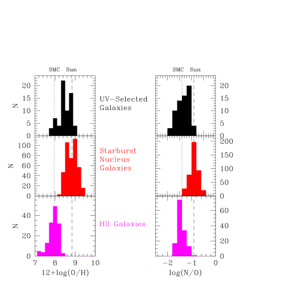
Figure 7: Distributions of left) the oxygen-to-hydrogen ($12+\log(\rm O/H)$) and right) nitrogen-to-oxygen (N/O) abundance ratios. The distribution of the UV-selected galaxy sample is compared to that of Starburst Nucleus Galaxies and Hii galaxies (see Fig. 9 for references). Abundance values for the Sun (dashed line) and for the SMC (dotted line) are indicated.

Table 1: Mean values and standard deviation of O/H and N/O abundance ratios for the UV-selected galaxies and comparison samples of local star-forming galaxies.

Sample	N	12+log(O/H)	log(N/O)
UV galaxies	68	8.49$\pm$ 0.04	$-$1.35$\pm$ 0.03
SBNGs	417	8.83$\pm$ 0.01	$-$0.90$\pm$ 0.01
Hii galaxies	139	7.91$\pm$ 0.02	$-$1.43$\pm$ 0.01

4.3 Systematic errors on N/O abundance ratios?

The quoted errors on O/H and N/O abundance ratios listed in Table 3 are uncertainties arising from measurement errors only and do not take into account systematic calibration errors. For the majority of the galaxies, the observational uncertainties are indeed dominant ($\ga 0.2$ dex). Nonetheless, it is appropriate to ask whether there may be systematic problems with the abundance determinations. Most notably, we may underestimate the underlying Balmer absorption strength in some galaxies. In this case, the extinction coefficient $c_{\rm H\beta}$ would be overestimated and the line strengths of “blue” emission lines over-corrected. This effect might lead to an underestimate of the N/O abundance ratio.

Balmer absorption strengths were directly measured in 55 galaxy spectra ($\sim$ 80% of the final sample), and are thus quite reliable, but the assumed absorption equivalent width of 2 Å for the other 13 galaxies could be incorrect. Fortunately, only one of these galaxies exhibits a particularly low N/O value. We conclude that our discussions in the following sections regarding UV-selected galaxies with low N/O values are not strongly affected by systematic errors on Balmer absorption.

5 Analysis

In this section, we use abundance ratios to constrain the physical characteristics of the UV-selected galaxies. We compare their chemical properties to those of various samples of normal and star-forming galaxies in the local universe and at intermediate redshifts.

As before, we consider local star-forming Hii galaxies and SBNGs (see Coziol et al. 1999 for the dichotomy). The Hii galaxy sample is a compilation of irregular and blue compact dwarf galaxy samples from Kobulnicky & Skillman (1996) and Izotov & Thuan (1999). The SBNG sample is a merger of an optically-selected (Contini et al. 1998; Considère et al. 2000) and far-infrared selected sample (Veilleux et al. 1995). Finally, we consider a small sample of intermediate-redshift ($0.1<z<0.5$) emission-line galaxies for which both O/H and N/O abundance ratios are available (Kobulnicky & Zaritsky 1999).

5.1 The N/O versus O/H relationship

Figure 8: Nitrogen-to-oxygen (N/O) abundance ratio as a function of oxygen abundance ($12+\log(\rm O/H)$) for the UV-selected sample. a) Abundance ratios are shown with error bars. Theoritical curves for a primary (dotted line), a secondary (dashed line), and a primary + secondary (solid line) production of nitrogen (Vila-Costas & Edmunds 1993) are shown. b) A distinction is made between cluster (star symbols) and field (circles) galaxies. Cluster galaxies are selected using the redshift ranges $0.021\leq z\leq 0.025$ for Coma, and $0.019\leq z\leq 0.023$ for Abell 1367. A further distinction is made between field galaxies at low redshift ($z<0.1$, empty circles) and at intermediate redshift ($z\geq 0.1$, filled circles).

The distributions of O/H and N/O abundance ratios for the UV-selected galaxies are shown in Figure 7, together with comparison samples of local star-forming galaxies. Corresponding mean values of O/H and N/O with their standard deviations are listed in Table 1.

Our UV galaxies span a wide range of oxygen abundances, from $12+\log(\rm O/H)$ $\sim$ 7.7 ($\sim$ 0.1 Z_⊙) to 9.0 ($\sim$ Z_⊙). In terms of metallicity, they are thus intermediate between low-mass Hii galaxies and massive SBNGs. The situation is quite similar for the N/O abundance ratios; however the mean value is closer to that of Hii galaxies (only 0.08 dex higher) than to that of the SBNGs ($\sim$ 0.45 dex lower). A closer look at Figure 7 shows that a significant fraction of the UV galaxies has rather low N/O abundance ratios (log(N/O) $<-1.7$). This appears to be one of the most distinctive properties of the UV-selected sample.

In Figure 8 and 9, we examine how the N/O abundance ratio varies with O/H. The behaviour of N/O with increasing metallicity offers clues about the chemical evolution history of the galaxies and the stellar populations responsible for producing oxygen and nitrogen.

The origin of nitrogen has been a subject of debate for some years. The basic nucleosynthesis process is well understood. Nitrogen is thought to be synthesized in the CNO processing during hydrogen burning. However the stars responsible remain uncertain. If oxygen and carbon are produced in previous generations, then nitrogen produced in new stars should be proportional to the initial heavy element abundance (i.e. secondary synthesis). N/O should increase linearly with O/H, and such a correlation is indeed observed in high-metallicity ($12+\log(\rm O/H)$ $>8.5$) Hii regions (see Fig. 9). On the other hand, if oxygen and carbon are produced in the same stars prior to the CNO cycle rather than in previous generations, then nitrogen production is independent of the initial heavy element abundance (primary synthesis). This regime seems to dominate at low metallicities ($12+\log(\rm O/H)$ $<8.0$; e.g., Matteucci & Tosi 1985; Matteucci 1986), for example in dwarf Hii galaxies where N/O exceeds the extrapolation of the linear trend present at high abundances and does not correlate with O/H (see Fig. 9).

Standard evolution models predict that secondary nitrogen synthesis can occur in stars of all masses, while primary nitrogen synthesis is usually thought to occur mainly in the convective envelope of intermediate-mass stars ($\sim 3-8$ M_⊙) during the AGB phase (e.g. Renzini & Voli 1981; van den Hoek & Groenewegen 1997; Henry, Edmunds & Köppen 2000). However considerable progress has recently been made in including rotational effects on the transport of elements and angular momentum in stellar interiors (see review by Maeder & Meynet 2000). In some massive stars the convective helium shell penetrates into the hydrogen layer resulting in the production of significant amounts of primary nitrogen (e.g., Maeder 2000). Thus both intermediate-mass and massive stars are potential primary nitrogen producers. Note that for intermediate-mass stars, the most recent models (e.g. Marigo 2001) find a nitrogen production similar to that of earlier models (e.g. Renzini & Voli 1981) at $Z\sim 0.2$ Z_⊙ but which decreases with increasing metallicity.

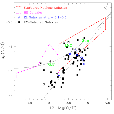
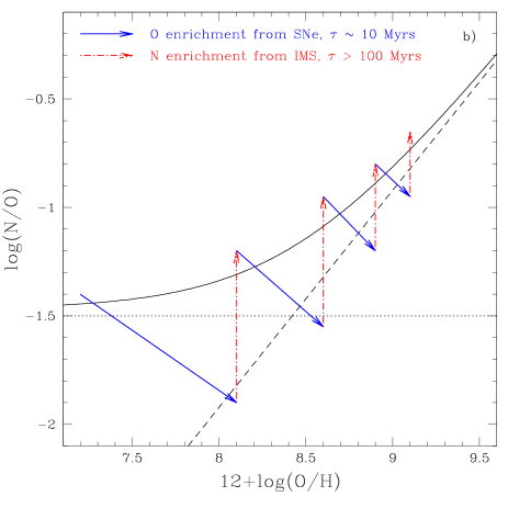
Figure 9: a) N/O versus $12+\log(\rm O/H)$ for the UV-selected galaxies (squares) and various comparison samples: Starburst Nucleus Galaxies (dot – short dash line) selected in the optical (Contini et al. 1998; Considère et al. 2000) or in the far-infrared (Veilleux et al. 1995), Hii galaxies (short dash – long dash line; Kobulnicky & Skillman 1996; Izotov & Thuan 1999), and a small sample of emission-line galaxies at intermediate redshift (stars; Kobulnicky & Zaritsky 1999). Empty squares denote UV-selected galaxies with two optical counterparts. Abundances ratios for the Sun, the LMC and the SMC are also indicated. b) Evolution model of N/O versus $12+\log(\rm O/H)$ assuming a sequence of starbursts separated by quiescent periods (see also Garnett 1990; Coziol et al. 1999). This scenario assumes that each burst first produces oxygen enrichment due to massive star evolution on short time-scales ($\tau\sim 10$ Myrs), followed by significant nitrogen enrichment on longer time-scales ($\tau>100$ Myrs) due to intermediate-mass star evolution (see text for details).

A major problem with N/O abundance ratios has been to explain the scatter in N/O at a given O/H (see Fig. 9). A natural explanation might be a significant time delay between the release of oxygen and that of nitrogen into the ISM (e.g., Edmunds & Pagel 1978; Garnett 1990; Pilyugin 1992, 1993, 1999; Vila-Costas & Edmunds 1993; Olofsson 1995b; Kobulnicky & Skillman 1996, 1998; Coziol et al. 1999). Chemical evolution models of galaxies producing stars in short bursts separated by long quiescent periods suggest that the dispersion in N/O could be due to a delayed release of nitrogen produced in low-mass longer-lived stars, compared to oxygen produced in massive, short-lived stars. The delayed-release hypothesis predicts that the N/O ratio evolves significantly during a single cycle of star formation followed by quiescence. Figure 9 illustrates this scenario. During a long period of quiescence, intermediate-mass star evolution will significantly enrich the galaxy in nitrogen but not in oxygen nor in any other Type II supernova product. At the end of a long quiescent period, the N/O ratio should be high and level out around $\log(\rm N/O)$ $\sim-1.5$ (e.g. Matteucci 1986; Olofsson 1995b), as a result of intermediate-mass star evolution over the last few hundred Myrs. During starburst however, N/O drops while O/H increases as the most massive stars begin to die and supernovae release oxygen into the ISM. A few tens of Myrs after the burst, the massive O stars producing oxygen will be gone. At this point, N/O should be minimal, with a value roughly limited by the yields of O and secondary N from the massive stars. Then N/O will rise again as intermediate-mass stars begin to contribute to the primary and secondary production of nitrogen, approaching a maximum value limited by the yields of N and O from all stars. A galaxy undergoing successive starbursts will thus oscillate between these two limits of N/O.

The vectors in Fig. 9 illustrate this evolution for a galaxy with an initial mass $10^{8}$ M_⊙, an initial metallicity $Z\sim 0.02$ Z_⊙, and $\log(\rm N/O)$ $\sim-1.5$, which converts 1% of its mass into massive stars (see Garnett 1990). Massive star evolution quickly moves the galaxy towards the lower right corner of the diagram. Ejection of nitrogen from intermediate-mass stars then increases N/O at constant O/H when the starburst has faded. A second burst moves the galaxy back towards the lower right corner, although to a lesser extent because of the higher abundance in the ISM. In this picture, the N/O ratio can be used as a “clock” to determine the time since the last major episode of star formation. The delayed-release hypothesis predicts that galaxies with high N/O ratios experienced a succession of starbursts separated by rather long quiescent intervals, and are preferentially picked out during a quiescent phase. On the other hand galaxies with low N/O ratios would have undergone shorter quiescent phases and would be picked out at the end of a strong episode of star-formation, when high-mass stars release large amounts of O into the ISM, while N is still withheld in lower-mass stars. Most of the UV-selected galaxies seem to fit this latter evolutionary scenario.

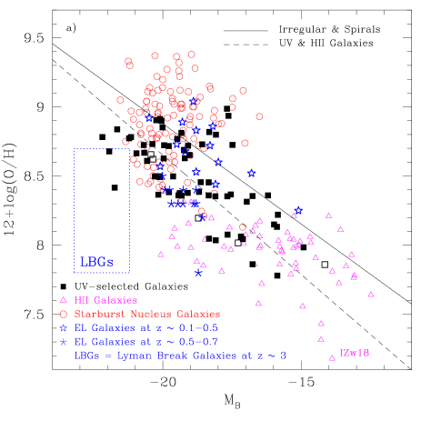
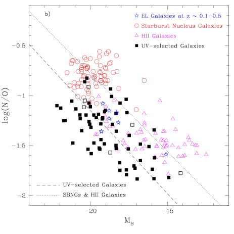
Figure 10: a) Metallicity–luminosity relation for the UV-selected sample (squares) and for comparison samples of local, intermediate and high redshift galaxies. The solid line is a linear least-squares fit to local irregular and spiral galaxies (see Kobulnicky & Zaritsky 1999). The local star-forming galaxy samples are the same as in Fig. 9: Hii galaxies (triangles) and SBNGs (circles). Two samples of intermediate-redshift galaxies (stars) are also shown for comparison: emission-line (EL) galaxies at $z\sim 0.1-0.5$ (Kobulnicky & Zaritsky 1999), and luminous compact EL galaxies at $z\sim 0.5-0.7$ (Hammer et al. 2001). The location of high-redshift ($z\sim 3$) Lyman break galaxies is shown as a box encompassing the range of O/H and $M_{\rm B}$ derived for these objects (Pettini et al. 2001). The dashed line is a mean least-squares fit to the UV-selected and Hii galaxies (correlation coefficient $r=-0.74$, rms $=0.26$). The slope of this relation ($=-0.173\pm 0.01$) is very close to the one derived for local irregular and spirals galaxies (solid line). UV-selected and Hii galaxies appear $2-3$ mag brighter than local “normal” galaxies of similar metallicity as might be expected if a strong starburst has temporarily lowered their mass-to-light ratios. b) N/O abundance ratio as a function of absolute $B$-band magnitude for the UV-selected sample (squares) and the comparison samples (see Fig. 9 for references). The dashed line is a mean least-squares fit to the UV-selected galaxies (correlation coefficient $r=-0.56$, rms $=0.21$). The dotted line is a mean least-squares fit to the SBNGs and Hii galaxies (correlation coefficient $r=-0.79$, rms $=0.22$). These two relations have nearly the same slope ($\sim-0.16$).

We can also investigate whether the chemical properties of UV-selected galaxies differ with environment – field galaxies vs. cluster galaxies – and with redshift – local galaxies ($z\la 0.1$) vs. intermediate-redshift galaxies ($z\ga 0.1$). In Figure 8b we differentiate between cluster galaxies (selected using the redshift ranges $0.021\leq z\leq 0.025$ for Coma, and $0.019\leq z\leq 0.023$ for Abell 1367) and the remaining sample, assumed to be field galaxies. No striking trends emerge, although there may be a tendency for high-metallicity ($12+\log(\rm O/H)$ $>8.7$) cluster galaxies to have lower N/O abundance ratios than their field counterparts. We also distinguish between low ($z<0.1$) and intermediate redshift ($z\geq 0.1$) field galaxies. The latter have relatively high oxygen abundances ($12+\log(\rm O/H)$ $>8.5$), some of them showing abundance properties typical of SBNGs with rather high N/O abundance ratios (log(N/O) $\ga-1$). This could be due to a succession of starbursts over the last few Gyrs (e.g. Coziol et al. 1999; Contini et al. 2000). The fact that UV galaxies at higher redshift are more metal-rich objects is likely to be a selection effect arising from the well-known metallicity–luminosity relationship (see Sect. 5.2).

Finally, we discuss two major sources of uncertainties in the delayed-release model. Firstly, the amount of gas and embedded metals lost by a galaxy due to supernova-driven superwinds is poorly constrained. If nitrogen is primary, then neither inflow of unprocessed gas nor outflow of enriched gas will affect the N/O ratio unless the outflow is different for nitrogen and oxygen (e.g. Pilyugin 1993; Marconi, Matteucci & Tosi 1994). If oxygen is predominantly synthesized in massive stars while nitrogen is produced in intermediate-mass stars, oxygen may be preferentially ejected during supernova explosions. If nitrogen is secondary, the N/O ratio is unaffected by any non-differential outflow, but can be affected by unprocessed gas inflow (Serrano & Peimbert 1983; Edmunds 1990; Köppen & Edmunds 1999).

Secondly, the time-scale for heavy element enrichment is still not well known. Since the nucleosynthetic products of massive stars require longer than $\sim 10$ Myrs to mix with the surrounding ISM (e.g., Tenorio-Tagle 1996; Kobulnicky & Skillman 1997), there will be some time lag ($>10$ Myrs) between supernova explosions and the appearance of fresh oxygen in the warm ionized gas. As long as this time lag is no longer than the lifetime of N-producing stars ($\sim$ some hundreds of Myrs), the N/O ratio may serve as a useful “clock” measuring the time elapsed since the last major burst of star formation. If however the time lag required for massive star ejecta to cool down and mix with the ISM is longer than a few $10^{8}$ yr, then the N/O ratio is unlikely to reflect accurately the time since the most recent starburst accurately. One test of the “clock” hypothesis would be to determine star formation histories across a wide range of N/O abundance ratios. Unfortunately, most of the galaxies in Figure 9 are too far away to directly investigate their star formation histories from stellar colour-magnitude diagrams.

5.2 Metallicity–luminosity relation

We now study how the UV-selected galaxies compare with the fundamental galaxy scaling relation between luminosity and metallicity (e.g., Lequeux et al. 1979; Brodie & Huchra 1991; Skillman, Kennicutt, & Hodge 1989; Zaritsky, Kennicutt & Huchra 1994; Richer & McCall 1995; Jablonka, Martin & Arimoto 1996; Coziol et al. 1997, 1998). This relation, which extends over $\sim 10$ magnitudes in luminosity and $\sim 2$ dex in metallicity, presumably reflects the fundamental role that galaxy mass plays in the chemical enrichment of the interstellar medium. The metallicity-luminosity relationship is usually attributed to the action of galactic superwinds; massive galaxies reach higher metallicities because they have deeper gravitational potentials better able to retain their gas against the building thermal pressures from supernovae, whereas low-mass systems eject their gas before high metallicities are attained (Larson 1974, De Young & Heckman 1994; Marlowe et al. 1995; MacLow & Ferrara 1999; Pilyugin & Ferrini 1998, 2000; Silich & Tenorio-Tagle 2001).

In Figure 10, the UV-selected sample is compared to i) local “normal” irregular and spiral galaxies, ii) nearby SBNGs and Hii galaxies, and iii) samples of intermediate and high redshift galaxies. The absolute $B$-band magnitudes of the UV-selected galaxies span seven orders of magnitude, from $M_{\rm B}$ $\sim-15$ to $-22$, with an average value $M_{\rm B}$ $=-18.8$ (Fig. 1a). In Figure 10 we distinguish between UV galaxies with one (filled squares) or two (empty squares) optical counterparts. The solid line is a linear fit to the metallicity-luminosity relation for local “normal” irregular and spiral galaxies (see Kobulnicky & Zaritsky 1999). Figure 10 includes samples of nearby Hii galaxies (Kobulnicky & Skillman 1996; Izotov & Thuan 1999) and SBNGs (Veilleux et al. 1995; Contini et al. 1998; Considère et al. 2000) discussed earlier. Absolute magnitudes for these were extracted from the LEDA database. Two samples of intermediate-redshift galaxies are also shown for comparison: emission-line galaxies at $z\sim 0.1-0.5$ (Kobulnicky & Zaritsky 1999), and luminous compact emission-line galaxies at $z\sim 0.5-0.7$ (Hammer et al. 2001). The location of high-redshift ($z\sim 3$) Lyman break galaxies is shown as a box encompassing the range of O/H and $M_{\rm B}$ derived for these objects (Pettini et al. 2001).

Figure 10a clearly shows that both UV-selected and Hii galaxies systematically deviate from the metallicity-luminosity trend of local “normal” galaxies (solid line). A mean least-squares fit (dashed line) to the UV-selected and Hii galaxies (obtained by fitting both samples independently and averaging the results) yields:

$$12+\log({\rm O/H})=-0.173(\pm 0.01)M_{\rm B}+5.195(\pm 0.177),$$ (10)

with a correlation coefficient $r=-0.74$, and a rms deviation of $0.26$. It is interesting to note that the slope of this relation is similar to the one derived for local “normal” galaxies. UV-selected and Hii galaxies thus appear $2-3$ mag brighter than “normal” galaxies of similar metallicity, as might be expected if a strong starburst has temporarily lowered their mass-to-light ratios. Note however that the departure of UV-selected galaxies from the metallicity-luminosity trend of local “normal” galaxies decreases with absolute magnitudes. Luminous ($M_{\rm B}$ $\sim-20$) UV-selected galaxies behave like low-metallicity SBNGs ($Z\la$ Z_⊙), which altogether do not follow the metallicity-luminosity relation. This could be understood in the context of accretion of residual outlying gas and/or small gas-rich galaxies. Following Struck-Marcell’s (1981) models, accretion of more gas than stars will result in a steepening of the metallicity-luminosity relation, explaining the behaviour of SBNGs and massive galaxies in general.

In Figure 10a, we also show the locus of intermediate ($z<1$) and high ($z\sim 3$) redshift objects. Whereas emission-line galaxies with redshifts between $0.1$ and $0.5$ follow the metallicity-luminosity relation of “normal” galaxies, there is a clear deviation for luminous and compact emission-line galaxies at higher redshift ($z\sim 0.5-0.7$). The latter objects better fit the metallicity-luminosity relation derived for UV-selected and Hii galaxies. Hammer et al. (2001) argue that these objects could be the progenitors of present-day spiral bulges. The deviation is even stronger for LBGs at $z\sim 3$. Even allowing for uncertainties in the determination of O/H and $M_{\rm B}$, LBGs fall well below the metallicity-luminosity relation of “normal” local galaxies and have much lower abundances than expected from this relation given their luminosities. The most obvious interpretation (Pettini et al. 2001) is that LBGs have mass-to-light ratios significantly lower than those of present-day “normal” galaxies.

Figure 10b shows the relation between N/O abundance ratio and absolute blue magnitude for the UV-selected and the comparison samples. Although the dispersion is higher than for the metallicity-luminosity relation, there is a clear correlation between $\log(\rm N/O)$ and $M_{\rm B}$. A mean least-squares fit (dashed line) to the UV-selected galaxies yields:

$$\log({\rm N/O})=-0.166(\pm 0.02)M_{\rm B}-4.472(\pm 0.275),$$ (11)

with a correlation coefficient $r=-0.56$, and a rms deviation of $0.21$. A similar relationship appears if we merge together the samples of SBNGs and Hii galaxies. A mean least-squares fit (dotted line) to these nearby star-forming galaxies yields:

$$\log({\rm N/O})=-0.156(\pm 0.01)M_{\rm B}-3.897(\pm 0.150),$$ (12)

with a correlation coefficient $r=-0.79$, and a rms deviation of $0.22$. It is interesting that these relations have nearly the same slope with a shift of $\sim 2-3$ mag in $M_{\rm B}$ or $\sim 0.4$ dex in $\log(\rm N/O)$. The rather low N/O abundance ratios in UV-selected galaxies compared with other star-forming galaxies is obvious in this plot. This supports the interpretation of the delayed-release model explained in section 5.1. We are witnessing UV-selected galaxies at a special stage of their evolution, just at the end of a powerful starburst which has suddenly enriched the ISM in oxygen and temporarily lowered their mass-to-light ratios. The fact that WR stars are not detected in the spectrum of UV-selected galaxies with low N/O values is another indication that the starburst is not young (age $\ga 10$ Myr) in these objects. On the other hand, the only galaxy with detected WR stars (see section 3.3), i.e. experiencing a rather young starburst, shows a high N/O abundance ratio ($\log(\rm N/O)$ $\sim-1.3$).

6 Conclusions

We examined the chemical properties of a sample of UV-selected intermediate-redshift ($0\la z\la 0.4$) galaxies in the context of their physical nature and star formation history. Our sample consists of 68 galaxies with heavy element abundance ratios, UV and CCD $B$-band photometry. The main results are the following:

• Diagnostics based on emission-line ratios show that all but one of the galaxies in our sample are powered by hot, young stars rather than by an AGN.

• Massive WR stars, indicating the presence of a very young starburst, are detected in only one UV galaxy. In particular, no WR spectral features were identified in the spectrum of galaxies with extreme UV-optical colours, refuting the claim that these hot stars could be responsible for this UV excess (Brown et al. 2000).

• UV-selected galaxies span a wide range of oxygen abundances, from $\sim$ 0.1 to 1 Z_⊙. They are intermediate between low-mass Hii galaxies and massive starburst nuclei, with no significant distinction between cluster and field galaxies.

• At a given oxygen abundance, the majority of the sample shows rather low N/O abundance ratios compared to other local samples of star-forming galaxies, such as Hii galaxies at low metallicities and SBNGs at higher metallicities. This is one of the most striking chemical properties of the UV-selected galaxies, allowing us to constrain their evolutionary stage in a new independent way (see below).

• Like Hii galaxies, UV-selected galaxies systematically deviate from the usual metallicity-luminosity relation. At a given metallicity they appear to be 2-3 magnitudes brighter than “normal” quiescent galaxies.

We examined the above results in the context of the “delayed-release” chemical evolution model. According to this model, most of the UV-selected galaxies recently experienced a powerful burst of star formation which temporarily lowered both their mass-to-light and N/O ratios. At this stage, intermediate-mass stars did not have enough time to evolve and release nitrogen, while the most massive stars have died and released their newly synthesized oxygen into the ISM through Type II supernova explosions. A significant number of massive stars must nevertheless still be present to account for the observed strong $\rm H{\alpha}$ emission lines (S2000).

If local UV galaxies represent scaled-down versions of the similarly UV-selected massive high-redshift LBGs, the present sample can be used to better understand the physical properties of these primordial galaxies. More quantitative chemical evolution modeling of these UV galaxies’ star formation history has been performed (Mouhcine & Contini 2001). Better quality spectra, near-infrared photometry as well as morphological informations should provide us with complementary observational constraints to probe deeper into the role of starbursts in galaxy formation and evolution.

Table 2: The sample of UV-selected galaxies with measurements of chemical abundances. Column 1 gives an ID number, columns 2 and 3 give the optical position (RA and DEC, 1950) of the objects. Column 4 indicates the number of optical counterparts (OC) on the POSS plates within 10″. Columns 5 to 10 list emission-line ratios used for standard diagnostic diagrams or as abundance indicators (see text for details). Column 11 indicates if the object lies on the lower (L) or on the upper (U) branch of the O/H vs. $R_{\rm 23}$ relationship, or falls in the turnaround region (?). Columns 12 and 13 give the oxygen abundance, $12+\log(\rm O/H)$, derived from the empirical calibrations (McGaugh 1991), on the lower and on the upper branch respectively.

#	RA (1950)	DEC (1950)	OC	[O iii]/[O ii]	[O iii]/$\rm H{\beta}$	[N i i]/$\rm H{\alpha}$	[S ii]/$\rm H{\alpha}$	[N ii]/[O ii]	log($R_{\rm 23}$)		O/HL	O/HU
(1)	(2)	(3)	(4)	(5)	(6)	(7)	(8)	(9)	(10)	(11)	(12)	(13)
1	13:06:32.16	$+$29:48:38.2	1	$-$0.85$\pm$ 0.19	$-$0.70$\pm$ 0.20	$-$0.56$\pm$ 0.10	$-$0.83$\pm$ 0.10	$-$0.25$\pm$ 0.10	0.25$\pm$ 0.15	U	7.49	8.99
2	13:06:46.29	$+$29:43:37.9	1	$-$0.42$\pm$ 0.25	0.08$\pm$ 0.25	$-$1.00$\pm$ 0.07	$-$0.30$\pm$ 0.08	$-$1.04$\pm$ 0.07	0.64$\pm$ 0.17	U	7.94	8.72
3	13:06:50.23	$+$29:40:26.7	2	$-$1.34$\pm$ 0.26	$-$0.83$\pm$ 0.34	$-$0.39$\pm$ 0.32		$-$0.45$\pm$ 0.30	0.55$\pm$ 0.22	U	8.05	8.77
4	13:06:30.66	$+$29:39:30.4	1	$-$0.41$\pm$ 0.18	0.32$\pm$ 0.25	$-$0.31$\pm$ 0.26		$-$0.59$\pm$ 0.25	0.91$\pm$ 0.26	U	8.35	8.39
5	13:06:07.74	$+$29:44:40.2	1	0.03$\pm$ 0.03	0.52$\pm$ 0.04	$-$1.43$\pm$ 0.20	$-$0.97$\pm$ 0.05	$-$1.46$\pm$ 0.20	0.87$\pm$ 0.03	L	8.13	8.51
6	13:06:07.65	$+$29:36:35.6	1	$-$1.03$\pm$ 0.24	$-$0.42$\pm$ 0.24	$-$0.45$\pm$ 0.21	$-$0.35$\pm$ 0.19	$-$0.61$\pm$ 0.22	0.66$\pm$ 0.17	U	8.15	8.66
7	13:07:05.26	$+$29:11:28.8	2	$-$0.32$\pm$ 0.04	0.31$\pm$ 0.06	$-$1.00$\pm$ 0.11	$-$0.49$\pm$ 0.05	$-$1.18$\pm$ 0.11	0.84$\pm$ 0.05	L	8.20	8.50
8	13:05:00.02	$+$29:40:04.3	1	0.06$\pm$ 0.03	0.62$\pm$ 0.03	$-$1.42$\pm$ 0.11	$-$0.77$\pm$ 0.03	$-$1.53$\pm$ 0.11	0.97$\pm$ 0.02	L	8.31	8.37
9	13:03:49.57	$+$29:58:56.5	1	$-$1.14$\pm$ 0.45	$-$0.64$\pm$ 0.46	$-$0.81$\pm$ 0.40		$-$0.87$\pm$ 0.37	0.54$\pm$ 0.32	U	8.03	8.78
10	13:06:48.52	$+$29:02:35.2	1	$-$0.18$\pm$ 0.06	0.42$\pm$ 0.10	$-$1.12$\pm$ 0.37		$-$1.26$\pm$ 0.37	0.89$\pm$ 0.09	L	8.22	8.46
11	13:04:13.54	$+$29:39:51.1	2	0.20$\pm$ 0.06	0.54$\pm$ 0.12	$-$1.02$\pm$ 0.22		$-$0.90$\pm$ 0.22	0.84$\pm$ 0.07	L	8.02	8.57
12	13:05:40.80	$+$29:14:43.1	1	$-$0.64$\pm$ 0.74	0.13$\pm$ 0.82	$-$0.91$\pm$ 0.82	$-$0.59$\pm$ 0.74	$-$1.23$\pm$ 0.80	0.88$\pm$ 0.61	?	8.37	8.40
13	13:04:37.54	$+$29:29:21.4	1	$-$0.61$\pm$ 0.08	$-$0.33$\pm$ 0.09	$-$0.30$\pm$ 0.05	$-$0.32$\pm$ 0.04	$-$0.13$\pm$ 0.05	0.41$\pm$ 0.06	U	7.65	8.90
14	13:03:37.14	$+$29:44:00.2	1	$-$0.79$\pm$ 0.17	$-$0.05$\pm$ 0.20	$-$0.49$\pm$ 0.17	$-$0.29$\pm$ 0.14	$-$0.78$\pm$ 0.17	0.83$\pm$ 0.16	U	8.33	8.45
15	13:03:48.44	$+$29:40:05.1	1	$-$0.13$\pm$ 0.03	0.27$\pm$ 0.04	$-$0.81$\pm$ 0.05	$-$0.52$\pm$ 0.03	$-$0.75$\pm$ 0.05	0.71$\pm$ 0.04	U	7.89	8.69
16	13:06:11.39	$+$29:00:41.8	1	$-$0.44$\pm$ 0.16	$-$0.05$\pm$ 0.26	$-$0.49$\pm$ 0.17	$-$0.25$\pm$ 0.15	$-$0.48$\pm$ 0.17	0.56$\pm$ 0.26	U	7.80	8.80
17	13:05:55.86	$+$29:02:53.4	1	$-$0.19$\pm$ 0.05	0.50$\pm$ 0.06	$-$1.20$\pm$ 0.11	$-$0.60$\pm$ 0.07	$-$1.43$\pm$ 0.11	0.96$\pm$ 0.04	L	8.35	8.35
18	13:02:53.21	$+$29:51:18.0	1	$-$0.31$\pm$ 0.07	0.22$\pm$ 0.11	$-$1.21$\pm$ 0.06	$-$0.83$\pm$ 0.12	$-$1.28$\pm$ 0.06	0.76$\pm$ 0.09	L	8.05	8.61
19	13:02:43.94	$+$29:52:15.3	1	$-$0.47$\pm$ 0.07	0.09$\pm$ 0.10	$-$0.64$\pm$ 0.11		$-$0.75$\pm$ 0.10	0.73$\pm$ 0.06	U	8.06	8.63
20	13:05:30.34	$+$29:03:16.3	2	$-$0.47$\pm$ 0.11	0.07$\pm$ 0.13	$-$0.54$\pm$ 0.09		$-$0.63$\pm$ 0.09	0.71$\pm$ 0.09	U	8.02	8.66
21	13:04:23.62	$+$29:15:48.9	1	$-$0.47$\pm$ 0.09	0.20$\pm$ 0.09	$-$0.65$\pm$ 0.08	$-$0.17$\pm$ 0.08	$-$0.87$\pm$ 0.09	0.84$\pm$ 0.08	U	8.23	8.49
22	13:03:28.24	$+$29:25:25.9	1	$-$0.70$\pm$ 0.14	$-$0.17$\pm$ 0.19	$-$0.58$\pm$ 0.13		$-$0.65$\pm$ 0.13	0.63$\pm$ 0.12	U	7.99	8.72
23	13:02:00.66	$+$29:47:57.0	1	$-$0.36$\pm$ 0.05	0.16$\pm$ 0.06	$-$0.60$\pm$ 0.07		$-$0.67$\pm$ 0.07	0.72$\pm$ 0.09	U	8.00	8.65
24	13:04:00.52	$+$29:14:47.2	2	$-$1.01$\pm$ 0.51	$-$0.28$\pm$ 0.46	$-$0.20$\pm$ 0.38	0.20$\pm$ 0.34	$-$0.48$\pm$ 0.44	0.78$\pm$ 0.34	U	8.33	8.50
25	13:04:50.67	$+$28:58:14.8	1	0.18$\pm$ 0.24	0.63$\pm$ 0.29	$-$0.62$\pm$ 0.20		$-$0.68$\pm$ 0.22	0.93$\pm$ 0.19	U	8.20	8.45
26	13:04:48.41	$+$28:54:49.3	1	$-$0.33$\pm$ 0.18	0.38$\pm$ 0.20	$-$0.92$\pm$ 0.18	$-$0.46$\pm$ 0.18	$-$1.17$\pm$ 0.18	0.91$\pm$ 0.14	?	8.32	8.40
27	13:04:19.78	$+$29:00:26.9	2	$-$0.17$\pm$ 0.13	0.35$\pm$ 0.13	$-$0.52$\pm$ 0.06	$-$0.51$\pm$ 0.06	$-$0.59$\pm$ 0.07	0.75$\pm$ 0.09	U	8.03	8.62
28	13:04:28.46	$+$28:57:50.8	1	$-$1.03$\pm$ 0.49	$-$0.23$\pm$ 0.50	$-$0.51$\pm$ 0.41		$-$0.86$\pm$ 0.46	0.84$\pm$ 0.35	U	8.41	8.42
29	13:01:41.32	$+$29:39:36.8	1	$-$0.51$\pm$ 0.08	$-$0.03$\pm$ 0.08	$-$0.30$\pm$ 0.09	$-$0.43$\pm$ 0.07	$-$0.32$\pm$ 0.09	0.63$\pm$ 0.08	U	7.91	8.73
30	13:02:56.12	$+$29:18:53.6	2	0.10$\pm$ 0.04	0.40$\pm$ 0.07	$-$1.47$\pm$ 0.35	$-$0.75$\pm$ 0.07	$-$1.31$\pm$ 0.36	0.73$\pm$ 0.05	L	7.86	8.68
31	13:03:21.92	$+$29:08:18.0	1	$-$0.40$\pm$ 0.05	0.17$\pm$ 0.11	$-$1.20$\pm$ 0.18	$-$0.54$\pm$ 0.05	$-$1.34$\pm$ 0.18	0.76$\pm$ 0.07	L	8.08	8.60
32	13:02:11.57	$+$29:25:28.0	1	$-$0.34$\pm$ 0.21	0.18$\pm$ 0.28	$-$1.21$\pm$ 0.23		$-$1.28$\pm$ 0.22	0.79$\pm$ 0.19	L	8.06	8.59
33	13:02:14.19	$+$29:21:01.9	1	$-$0.32$\pm$ 0.04	0.40$\pm$ 0.04	$-$0.85$\pm$ 0.08	$-$0.65$\pm$ 0.05	$-$1.12$\pm$ 0.08	0.94$\pm$ 0.04	?	8.36	8.36
34	13:02:47.46	$+$29:07:09.6	1	$-$0.40$\pm$ 0.12	0.37$\pm$ 0.12	$-$0.88$\pm$ 0.14		$-$1.20$\pm$ 0.14	0.94$\pm$ 0.09	?	8.36	8.36
35	13:02:15.16	$+$29:14:25.5	1	$-$0.23$\pm$ 0.09	0.53$\pm$ 0.12	$-$1.05$\pm$ 0.15	$-$0.90$\pm$ 0.11	$-$1.36$\pm$ 0.15	0.96$\pm$ 0.08	L	8.35	8.35
36	13:02:45.39	$+$29:04:56.9	1	$-$1.15$\pm$ 0.41	$-$0.71$\pm$ 0.43	$-$0.61$\pm$ 0.27		$-$0.60$\pm$ 0.28	0.48$\pm$ 0.30	U	7.94	8.84
37	13:00:49.01	$+$29:34:15.4	1	$-$0.83$\pm$ 0.37	$-$0.11$\pm$ 0.38	$-$0.52$\pm$ 0.34		$-$0.78$\pm$ 0.35	0.80$\pm$ 0.29	U	8.28	8.50
38	13:00:53.53	$+$29:31:42.1	1	$-$1.09$\pm$ 0.22	$-$0.45$\pm$ 0.23	$-$0.63$\pm$ 0.18		$-$0.81$\pm$ 0.18	0.68$\pm$ 0.16	U	8.21	8.63
39	13:03:48.16	$+$28:43:55.0	1	$-$0.44$\pm$ 0.08	0.28$\pm$ 0.09	$-$0.92$\pm$ 0.10	$-$0.58$\pm$ 0.07	$-$1.18$\pm$ 0.10	0.89$\pm$ 0.06	?	8.32	8.41
40	13:03:45.03	$+$28:43:35.2	1	$-$0.67$\pm$ 0.05	$-$0.06$\pm$ 0.06	$-$0.72$\pm$ 0.05	$-$0.58$\pm$ 0.04	$-$0.88$\pm$ 0.05	0.73$\pm$ 0.06	U	8.12	8.61
41	13:02:51.82	$+$28:53:38.2	1	$-$0.46$\pm$ 0.08	0.31$\pm$ 0.10	$-$0.88$\pm$ 0.09	$-$0.67$\pm$ 0.09	$-$1.20$\pm$ 0.10	0.92$\pm$ 0.06	?	8.37	8.37
42	13:00:59.29	$+$29:22:49.2	1	$-$0.35$\pm$ 0.13	0.03$\pm$ 0.20	$-$0.71$\pm$ 0.19		$-$0.63$\pm$ 0.17	0.61$\pm$ 0.17	U	7.80	8.77
43	13:02:42.78	$+$28:54:32.0	1	$-$0.25$\pm$ 0.08	0.47$\pm$ 0.11	$-$1.07$\pm$ 0.13	$-$0.59$\pm$ 0.09	$-$1.34$\pm$ 0.12	0.95$\pm$ 0.07	L	8.35	8.35
44	13:01:53.07	$+$29:07:07.0	1	0.08$\pm$ 0.01	0.56$\pm$ 0.03	$-$1.36$\pm$ 0.11	$-$0.98$\pm$ 0.05	$-$1.38$\pm$ 0.11	0.89$\pm$ 0.01	L	8.15	8.49
45	13:01:59.06	$+$29:04:42.8	1	$-$0.70$\pm$ 0.06	0.09$\pm$ 0.06	$-$0.77$\pm$ 0.07	$-$0.50$\pm$ 0.07	$-$1.12$\pm$ 0.07	0.89$\pm$ 0.05	?	8.38	8.38
46	13:02:05.41	$+$29:01:54.8	1	$-$0.23$\pm$ 0.08	0.24$\pm$ 0.11	$-$1.25$\pm$ 0.26		$-$1.36$\pm$ 0.26	0.75$\pm$ 0.07	L	7.99	8.64
47	13:01:58.51	$+$29:01:55.0	2	0.24$\pm$ 0.09	0.65$\pm$ 0.20	$-$0.91$\pm$ 0.55		$-$0.87$\pm$ 0.55	0.94$\pm$ 0.12	U	8.19	8.46
48	13:02:25.99	$+$28:51:14.9	1	$-$0.28$\pm$ 0.06	0.34$\pm$ 0.11	$-$0.67$\pm$ 0.13		$-$0.83$\pm$ 0.13	0.85$\pm$ 0.06	U	8.19	8.50
49	13:02:11.95	$+$28:53:43.2	1	$-$0.64$\pm$ 0.10	0.14$\pm$ 0.11	$-$0.80$\pm$ 0.10	$-$0.60$\pm$ 0.11	$-$1.13$\pm$ 0.11	0.90$\pm$ 0.09	?	8.38	8.38
50	13:02:41.80	$+$28:42:17.0	1	$-$0.91$\pm$ 0.12	$-$0.42$\pm$ 0.12	$-$0.47$\pm$ 0.13	$-$0.73$\pm$ 0.15	$-$0.50$\pm$ 0.13	0.55$\pm$ 0.09	U	7.96	8.78
51	13:02:33.29	$+$28:43:05.3	1	$-$0.66$\pm$ 0.18	$-$0.15$\pm$ 0.18	$-$0.56$\pm$ 0.17		$-$0.62$\pm$ 0.15	0.63$\pm$ 0.19	U	7.97	8.72
52	13:01:49.26	$+$28:48:37.7	1	$-$0.03$\pm$ 0.10	0.32$\pm$ 0.14	$-$1.00$\pm$ 0.10		$-$1.00$\pm$ 0.10	0.70$\pm$ 0.10	L	7.86	8.70
53	13:01:07.18	$+$28:57:30.8	1	0.19$\pm$ 0.09	0.40$\pm$ 0.23	$-$1.10$\pm$ 0.08		$-$0.86$\pm$ 0.08	0.71$\pm$ 0.14	L	7.78	8.72
54	11:40:59.21	$+$20:46:04.6	1	$-$1.03$\pm$ 0.18	$-$0.44$\pm$ 0.18	$-$0.46$\pm$ 0.09	$-$0.54$\pm$ 0.09	$-$0.60$\pm$ 0.11	0.65$\pm$ 0.15	U	8.11	8.68
55	11:41:26.28	$+$20:39:30.9	1	$-$0.61$\pm$ 0.14	0.12$\pm$ 0.14	$-$0.88$\pm$ 0.16	$-$0.48$\pm$ 0.12	$-$1.15$\pm$ 0.17	0.85$\pm$ 0.10	?	8.31	8.45
56	11:41:13.29	$+$20:31:34.6	1	$-$0.43$\pm$ 0.01	0.04$\pm$ 0.01	$-$0.73$\pm$ 0.01	$-$1.02$\pm$ 0.02	$-$0.75$\pm$ 0.01	0.64$\pm$ 0.01	U	7.91	8.73
57	11:43:04.16	$+$20:22:49.6	1	$-$1.19$\pm$ 0.20	$-$0.58$\pm$ 0.21	$-$0.54$\pm$ 0.18		$-$0.70$\pm$ 0.17	0.64$\pm$ 0.14	U	8.19	8.67
58	11:41:22.60	$+$20:27:44.9	1	$-$1.09$\pm$ 0.20	$-$0.74$\pm$ 0.19	$-$0.68$\pm$ 0.14	$-$0.90$\pm$ 0.12	$-$0.59$\pm$ 0.15	0.40$\pm$ 0.14	U	7.82	8.90
59	11:41:56.61	$+$20:23:02.9	1	$-$1.07$\pm$ 0.16	$-$0.66$\pm$ 0.14	$-$0.49$\pm$ 0.12	$-$0.76$\pm$ 0.13	$-$0.46$\pm$ 0.13	0.47$\pm$ 0.12	U	7.86	8.85
60	11:40:48.41	$+$20:25:49.3	1	$-$0.26$\pm$ 0.02	0.27$\pm$ 0.03	$-$1.02$\pm$ 0.08	$-$0.76$\pm$ 0.04	$-$1.09$\pm$ 0.08	0.77$\pm$ 0.03	L	8.05	8.60
61	11:41:01.40	$+$20:21:04.4	1	0.00$\pm$ 0.01	0.44$\pm$ 0.02	$-$1.35$\pm$ 0.07	$-$0.59$\pm$ 0.04	$-$1.34$\pm$ 0.07	0.81$\pm$ 0.01	L	8.03	8.58
62	11:39:39.87	$+$20:19:34.2	1	$-$0.55$\pm$ 0.08	$-$0.36$\pm$ 0.11	$-$0.71$\pm$ 0.06	$-$0.63$\pm$ 0.03	$-$0.45$\pm$ 0.06	0.36$\pm$ 0.09	U	7.53	8.94
63	11:42:19.65	$+$20:09:28.8	1	$-$1.02$\pm$ 0.46	$-$0.47$\pm$ 0.50	$-$0.53$\pm$ 0.35		$-$0.63$\pm$ 0.39	0.60$\pm$ 0.34	U	8.07	8.72
64	11:40:20.70	$+$20:14:37.2	1	$-$0.87$\pm$ 0.09	$-$0.45$\pm$ 0.09	$-$0.77$\pm$ 0.07	$-$0.71$\pm$ 0.07	$-$0.74$\pm$ 0.07	0.52$\pm$ 0.07	U	7.84	8.82
65	11:40:03.61	$+$20:14:47.5	1	$-$0.50$\pm$ 0.06	$-$0.02$\pm$ 0.07	$-$0.84$\pm$ 0.06	$-$0.69$\pm$ 0.06	$-$0.86$\pm$ 0.06	0.64$\pm$ 0.05	U	7.92	8.73
66	11:40:18.41	$+$20:13:05.5	1	$-$0.35$\pm$ 0.19	0.42$\pm$ 0.22	$-$0.86$\pm$ 0.27		$-$1.17$\pm$ 0.27	0.94$\pm$ 0.14	?	8.36	8.36
67	11:42:27.23	$+$20:02:00.1	1	$-$0.79$\pm$ 0.19	$-$0.52$\pm$ 0.19	$-$0.55$\pm$ 0.13	$-$0.64$\pm$ 0.12	$-$0.37$\pm$ 0.13	0.40$\pm$ 0.16	U	7.63	8.91
68	11:41:26.36	$+$20:03:43.3	1	$-$0.98$\pm$ 0.15	$-$0.52$\pm$ 0.14	$-$0.65$\pm$ 0.11	$-$0.48$\pm$ 0.10	$-$0.66$\pm$ 0.11	0.52$\pm$ 0.10	U	7.93	8.81

Table 3: The sample of UV-selected galaxies with measurements of chemical abundances. Column 1 gives an ID number, columns 2 and 3 give the optical position (RA and DEC, 1950) of the objects. Column 4 indicates the number of optical counterparts (OC) on the POSS plates within 10″. Column 5 gives the redshift. Column 6 gives the extinction coefficient $A_{\rm v}$. Columns 7 and 8 give the O/H and N/O abundances ratios with their uncertainties.

#	RA (1950)	DEC (1950)	OC	z	$A_{\rm V}$	12+log(O/H)	log(N/O)
(1)	(2)	(3)	(4)	(5)	(6)	(7)	(8)
1	13:06:32.16	$+$29:48:38.2	1	0.023	0.57$\pm$ 0.06	8.99$\pm$ 0.37	$-$1.04$\pm$ 0.14
2	13:06:46.29	$+$29:43:37.9	1	0.113	0.85$\pm$ 0.07	8.72$\pm$ 0.27	$-$1.58$\pm$ 0.21
3	13:06:50.23	$+$29:40:26.7	2	0.243	0.98$\pm$ 0.27	8.77$\pm$ 0.30	$-$1.05$\pm$ 0.25
4	13:06:30.66	$+$29:39:30.4	1	0.228	0.52$\pm$ 0.15	8.39$\pm$ 0.48	$-$0.93$\pm$ 0.35
5	13:06:07.74	$+$29:44:40.2	1	0.024	0.57$\pm$ 0.03	8.13$\pm$ 0.07	$-$1.83$\pm$ 0.04
6	13:06:07.65	$+$29:36:35.6	1	0.123	1.85$\pm$ 0.19	8.66$\pm$ 0.26	$-$1.13$\pm$ 0.21
7	13:07:05.26	$+$29:11:28.8	2	0.063	0.61$\pm$ 0.04	8.20$\pm$ 0.13	$-$1.57$\pm$ 0.06
8	13:05:00.02	$+$29:40:04.3	1	0.018	0.78$\pm$ 0.03	8.31$\pm$ 0.06	$-$1.84$\pm$ 0.03
9	13:03:49.57	$+$29:58:56.5	1	0.335	2.27$\pm$ 0.37	8.78$\pm$ 0.47	$-$1.48$\pm$ 0.37
10	13:06:48.52	$+$29:02:35.2	1	0.021	0.13$\pm$ 0.03	8.22$\pm$ 0.25	$-$1.62$\pm$ 0.20
11	13:04:13.54	$+$29:39:51.1	2	0.090	0.33$\pm$ 0.04	8.02$\pm$ 0.17	$-$1.29$\pm$ 0.16
12	13:05:40.80	$+$29:14:43.1	1	0.080	2.44$\pm$ 0.77	8.38$\pm$ 1.02	$-$1.60$\pm$ 0.40
13	13:04:37.54	$+$29:29:21.4	1	0.167	0.35$\pm$ 0.03	8.90$\pm$ 0.17	$-$0.83$\pm$ 0.07
14	13:03:37.14	$+$29:44:00.2	1	0.051	0.81$\pm$ 0.12	8.45$\pm$ 0.26	$-$1.18$\pm$ 0.20
15	13:03:48.44	$+$29:40:05.1	1	0.182	0.15$\pm$ 0.01	8.69$\pm$ 0.11	$-$1.23$\pm$ 0.04
16	13:06:11.39	$+$29:00:41.8	1	0.056	0.00$\pm$ 0.13	8.80$\pm$ 0.39	$-$1.08$\pm$ 0.32
17	13:05:55.86	$+$29:02:53.4	1	0.039	1.20$\pm$ 0.06	8.35$\pm$ 0.13	$-$1.74$\pm$ 0.05
18	13:02:53.21	$+$29:51:18.0	1	0.024	0.39$\pm$ 0.06	8.05$\pm$ 0.21	$-$1.73$\pm$ 0.11
19	13:02:43.94	$+$29:52:15.3	1	0.185	0.61$\pm$ 0.07	8.63$\pm$ 0.20	$-$1.22$\pm$ 0.08
20	13:05:30.34	$+$29:03:16.3	2	0.248	1.79$\pm$ 0.10	8.66$\pm$ 0.26	$-$1.12$\pm$ 0.10
21	13:04:23.62	$+$29:15:48.9	1	0.062	1.18$\pm$ 0.09	8.49$\pm$ 0.25	$-$1.26$\pm$ 0.09
22	13:03:28.24	$+$29:25:25.9	1	0.242	0.61$\pm$ 0.12	8.72$\pm$ 0.35	$-$1.20$\pm$ 0.14
23	13:02:00.66	$+$29:47:57.0	1	0.223	0.57$\pm$ 0.04	8.65$\pm$ 0.31	$-$1.15$\pm$ 0.12
24	13:04:00.52	$+$29:14:47.2	2	0.285	1.77$\pm$ 0.41	8.50$\pm$ 0.54	$-$0.91$\pm$ 0.23
25	13:04:50.67	$+$28:58:14.8	1	0.247	0.00$\pm$ 0.21	8.45$\pm$ 0.38	$-$1.01$\pm$ 0.29
26	13:04:48.41	$+$28:54:49.3	1	0.040	0.87$\pm$ 0.19	8.36$\pm$ 0.25	$-$1.51$\pm$ 0.19
27	13:04:19.78	$+$29:00:26.9	2	0.113	1.09$\pm$ 0.04	8.62$\pm$ 0.31	$-$1.05$\pm$ 0.12
28	13:04:28.46	$+$28:57:50.8	1	0.388	2.07$\pm$ 0.49	8.42$\pm$ 0.56	$-$1.25$\pm$ 0.23
29	13:01:41.32	$+$29:39:36.8	1	0.167	0.96$\pm$ 0.07	8.73$\pm$ 0.25	$-$0.86$\pm$ 0.10
30	13:02:56.12	$+$29:18:53.6	2	0.018	0.33$\pm$ 0.03	7.86$\pm$ 0.11	$-$1.78$\pm$ 0.08
31	13:03:21.92	$+$29:08:18.0	1	0.026	0.00$\pm$ 0.04	8.08$\pm$ 0.17	$-$1.79$\pm$ 0.09
32	13:02:11.57	$+$29:25:28.0	1	0.090	0.63$\pm$ 0.16	8.06$\pm$ 0.23	$-$1.71$\pm$ 0.25
33	13:02:14.19	$+$29:21:01.9	1	0.180	1.13$\pm$ 0.04	8.36$\pm$ 0.12	$-$1.44$\pm$ 0.04
34	13:02:47.46	$+$29:07:09.6	1	0.178	1.48$\pm$ 0.12	8.36$\pm$ 0.30	$-$1.52$\pm$ 0.11
35	13:02:15.16	$+$29:14:25.5	1	0.025	1.07$\pm$ 0.10	8.35$\pm$ 0.26	$-$1.67$\pm$ 0.10
36	13:02:45.39	$+$29:04:56.9	1	0.186	1.48$\pm$ 0.25	8.84$\pm$ 0.42	$-$1.25$\pm$ 0.33
37	13:00:49.01	$+$29:34:15.4	1	0.083	1.74$\pm$ 0.36	8.50$\pm$ 0.49	$-$1.20$\pm$ 0.38
38	13:00:53.53	$+$29:31:42.1	1	0.082	1.40$\pm$ 0.21	8.63$\pm$ 0.24	$-$1.32$\pm$ 0.20
39	13:03:48.16	$+$28:43:55.0	1	0.068	0.98$\pm$ 0.07	8.36$\pm$ 0.20	$-$1.54$\pm$ 0.08
40	13:03:45.03	$+$28:43:35.2	1	0.068	1.22$\pm$ 0.04	8.61$\pm$ 0.19	$-$1.35$\pm$ 0.07
41	13:02:51.82	$+$28:53:38.2	1	0.022	1.22$\pm$ 0.09	8.37$\pm$ 0.22	$-$1.53$\pm$ 0.08
42	13:00:59.29	$+$29:22:49.2	1	0.083	0.50$\pm$ 0.13	8.77$\pm$ 0.25	$-$1.19$\pm$ 0.20
43	13:02:42.78	$+$28:54:32.0	1	0.018	1.22$\pm$ 0.09	8.35$\pm$ 0.23	$-$1.65$\pm$ 0.09
44	13:01:53.07	$+$29:07:07.0	1	0.025	0.39$\pm$ 0.01	8.15$\pm$ 0.04	$-$1.74$\pm$ 0.02
45	13:01:59.06	$+$29:04:42.8	1	0.027	1.26$\pm$ 0.06	8.38$\pm$ 0.15	$-$1.47$\pm$ 0.06
46	13:02:05.41	$+$29:01:54.8	1	0.027	0.00$\pm$ 0.07	7.99$\pm$ 0.16	$-$1.82$\pm$ 0.11
47	13:01:58.51	$+$29:01:55.0	2	0.018	0.22$\pm$ 0.06	8.46$\pm$ 0.25	$-$1.19$\pm$ 0.34
48	13:02:25.99	$+$28:51:14.9	1	0.253	0.39$\pm$ 0.06	8.50$\pm$ 0.24	$-$1.22$\pm$ 0.09
49	13:02:11.95	$+$28:53:43.2	1	0.022	1.44$\pm$ 0.12	8.38$\pm$ 0.28	$-$1.48$\pm$ 0.11
50	13:02:41.80	$+$28:42:17.0	1	0.219	1.87$\pm$ 0.13	8.78$\pm$ 0.25	$-$1.10$\pm$ 0.10
51	13:02:33.29	$+$28:43:05.3	1	0.070	1.07$\pm$ 0.15	8.72$\pm$ 0.28	$-$1.16$\pm$ 0.22
52	13:01:49.26	$+$28:48:37.7	1	0.027	0.00$\pm$ 0.10	7.86$\pm$ 0.21	$-$1.49$\pm$ 0.13
53	13:01:07.18	$+$28:57:30.8	1	0.022	0.26$\pm$ 0.07	7.78$\pm$ 0.25	$-$1.34$\pm$ 0.17
54	11:40:59.21	$+$20:46:04.6	1	0.169	1.87$\pm$ 0.10	8.68$\pm$ 0.23	$-$1.13$\pm$ 0.19
55	11:41:26.28	$+$20:39:30.9	1	0.040	1.50$\pm$ 0.13	8.38$\pm$ 0.34	$-$1.54$\pm$ 0.14
56	11:41:13.29	$+$20:31:34.6	1	0.021	1.55$\pm$ 0.01	8.73$\pm$ 0.04	$-$1.29$\pm$ 0.01
57	11:43:04.16	$+$20:22:49.6	1	0.383	1.81$\pm$ 0.13	8.67$\pm$ 0.22	$-$1.23$\pm$ 0.18
58	11:41:22.60	$+$20:27:44.9	1	0.022	1.90$\pm$ 0.15	8.90$\pm$ 0.38	$-$1.29$\pm$ 0.14
59	11:41:56.61	$+$20:23:02.9	1	0.024	2.81$\pm$ 0.12	8.85$\pm$ 0.34	$-$1.11$\pm$ 0.14
60	11:40:48.41	$+$20:25:49.3	1	0.071	0.31$\pm$ 0.01	8.05$\pm$ 0.06	$-$1.53$\pm$ 0.03
61	11:41:01.40	$+$20:21:04.4	1	0.068	0.44$\pm$ 0.01	8.03$\pm$ 0.04	$-$1.75$\pm$ 0.02
62	11:39:39.87	$+$20:19:34.2	1	0.020	0.02$\pm$ 0.00	8.94$\pm$ 0.25	$-$1.17$\pm$ 0.10
63	11:42:19.65	$+$20:09:28.8	1	0.082	2.14$\pm$ 0.44	8.72$\pm$ 0.50	$-$1.19$\pm$ 0.20
64	11:40:20.70	$+$20:14:37.2	1	0.024	0.78$\pm$ 0.06	8.82$\pm$ 0.19	$-$1.36$\pm$ 0.08
65	11:40:03.61	$+$20:14:47.5	1	0.024	1.13$\pm$ 0.06	8.73$\pm$ 0.16	$-$1.40$\pm$ 0.06
66	11:40:18.41	$+$20:13:05.5	1	0.132	0.96$\pm$ 0.18	8.36$\pm$ 0.26	$-$1.50$\pm$ 0.19
67	11:42:27.23	$+$20:02:00.1	1	0.069	1.31$\pm$ 0.12	8.91$\pm$ 0.21	$-$1.08$\pm$ 0.16
68	11:41:26.36	$+$20:03:43.3	1	0.016	2.09$\pm$ 0.12	8.81$\pm$ 0.30	$-$1.28$\pm$ 0.12

References

- [1] Alloin D., Collin-Souffrin S., Joly M., Vigroux, L., 1979, A&A, 78, 200
- [2] Brodie J. P., Huchra J. P., 1991, ApJ, 379, 157
- [3] Brown W. R., Kenyon S. J., Geller M. J., Fabricant D. G., 2000, ApJ, 540, L83
- [4] Calzetti D., 1997, AJ, 113, 162
- [5] Carollo C. M., Lilly S. J., 2001, ApJ, 548, L153
- [6] Cole S., Lacey C. G., Baugh C. M., Frenk C. S., 2000, MNRAS, 319, 168
- [7] Considère S., Coziol R., Contini T., Davoust, E., 2000, A&A, 356, 89
- [8] Conti P. S., 1991, ApJ, 377, 115
- [9] Conti P. S., Leitherer C., Vacca W. D., 1996, ApJ, 461, L87
- [10] Contini T., Considère S., Davoust E., 1998, A&AS, 130, 285
- [11] Contini T., Coziol R., Considère S., Davoust E., Reyes R. E. C., 2000, in “Building Galaxies: From the Primordial Universe to the Present”, 34th Moriond Meeting, F. Hammer et al. (Editions Frontieres), p. 229 (astro-ph/9812410)
- [12] Contini T., Davoust E., Considère S., 1995, A&A, 303, 440
- [13] Coziol R., Contini T., Davoust E., Considère S., 1997, ApJ, 481, L67
- [14] Coziol R., Contini T., Davoust E., Considère S., 1998, ASP Conf. Ser. 147: Abundance Profiles: Diagnostic Tools for Galaxy History, p. 219
- [15] Coziol R., Reyes R. E. C., Considère S., Davoust E., Contini T., 1999, A&A, 345, 733
- [16] De Young D. S., Heckman T. M., 1994, ApJ, 431, 598
- [17] Dopita M. A., Evans I. N., 1986, ApJ, 307, 431
- [18] Dopita M. A., Kewley L. J., Heisler C. A., Sutherland R. S., 2000, ApJ, 542, 224
- [19] Edmunds M. G., 1990, MNRAS, 246, 678
- [20] Edmunds M. G., Pagel B. E. J., 1978, MNRAS, 185, 77
- [21] Edmunds M. G., Pagel B. E. J., 1984, MNRAS, 211, 507
- [22] Franx M., Illingworth G. D., Kelson D. D., van Dokkum P. G., Tran K., 1997, ApJ, 486, L75
- [23] Garnett D. R., 1990, ApJ, 363, 142
- [24] González Delgado R. M., Leitherer C., Heckman T. M., 1999, ApJS, 125, 489
- [25] Guseva N. G., Izotov Y. I., Thuan T. X., 2000, ApJ, 531, 776
- [26] Hammer F., Gruel N., Thuan T. X., Flores H., Infante L., 2001, ApJ, 550, 570
- [27] Heckman T. M., Robert C., Leitherer C., Garnett D. R., van der Rydt F., 1998, ApJ, 503, 646
- [28] Henry R. B. C., Edmunds M. G., Köppen J., 2000, ApJ, 541, 660
- [29] Izotov Y. I., Thuan T. X., 1998, ApJ, 500, 188
- [30] Izotov Y. I., Thuan T. X., 1999, ApJ, 511, 639
- [31] Izotov Y. I., Thuan T. X., Lipovetsky V. A., 1994, ApJ, 435, 647
- [32] Izotov Y. I., Thuan T. X., Lipovetsky V. A., 1997, ApJS, 108, 1
- [33] Jablonka P., Martin P., Arimoto N., 1996, AJ, 112, 1415
- [34] Kewley L. J., Heisler C. A., Dopita M. A., Lumsden S., 2001, ApJS, 132, 37
- [35] Kauffmann G., Charlot S., 1998, MNRAS, 294, 705
- [36] Kauffmann G., Charlot S., Balogh M. L., 2001, Apj in press (astro-ph/0103130)
- [37] Kobulnicky H. A., Kennicutt R. C., Pizagno J. L., 1999, ApJ, 514, 544
- [38] Kobulnicky H. A., Koo D. C., 2000, ApJ, 545, 712
- [39] Kobulnicky H. A., Skillman E. D., 1996, ApJ, 471, 211
- [40] Kobulnicky H. A., Skillman E. D., 1997, ApJ, 489, 636
- [41] Kobulnicky H. A., Skillman E. D., 1998, ApJ, 497, 601
- [42] Kobulnicky H. A., Zaritsky D., 1999, ApJ, 511, 118
- [43] Köppen J., Edmunds M. G., 1999, MNRAS, 306, 317
- [44] Kunth D., Mas-Hesse J. M., Terlevich E., Terlevich R., Lequeux J., Fall S. M., 1998, A&A, 334, 11
- [45] Larson R. B., 1974, MNRAS, 169, 229
- [46] Leitherer C., et al., 1999, ApJS, 123, 3
- [47] Lequeux J., Rayo J. F., Serrano A., Peimbert M., Torres-Peimbert S., 1979, A&A, 80, 155
- [48] Lilly S. J., Le Fevre O., Crampton D., Hammer F., Tresse L., 1995, ApJ, 455, 50
- [49] Lowenthal J. D., et al., 1997, ApJ, 481, 673
- [50] Mac Low M., Ferrara A., 1999, ApJ, 513, 142
- [51] Madau P., Pozzetti L., Dickinson M., 1998, ApJ, 498, 106
- [52] Maeder A., 2000, New Astronomy Review, 44, 291
- [53] Maeder A., Meynet G., 1994, A&A, 287, 803
- [54] Maeder A., Meynet G., 2000, ARA&A, 38, 143
- [55] Marigo P., 2001, A&A, 370, 194
- [56] Marconi G., Matteucci F., Tosi M., 1994, MNRAS, 270, 35
- [57] Marlowe A. T., Heckman T. M., Wyse R. F. G., Schommer R., 1995, ApJ, 438, 563
- [58] Matteucci F., 1986, MNRAS, 221, 911
- [59] Matteucci F., Tosi M., 1985, MNRAS, 217, 391
- [60] McCall M. L., Rybski P. M., Shields G. A. 1985, ApJS, 57, 1
- [61] McGaugh S. S., 1991, ApJ, 380, 140
- [62] McGaugh S. S., 1994, ApJ, 426, 135
- [63] Meurer G. R., Heckman T. M., Calzetti D., 1999, ApJ, 521, 64
- [64] Meurer G. R., Heckman T. M., Lehnert M. D., Leitherer C., Lowenthal J., 1997, AJ, 114, 54
- [65] Meynet G., 1995, A&A, 298, 767
- [66] Milliard B., Donas J., Laget M., Armand C., Vuillemin A., 1992, A&A, 257, 24
- [67] Mouhcine M., Contini T., 2001, A&A, submitted
- [68] Olofsson K., 1995a, A&AS, 111, 57
- [69] Olofsson K., 1995b, A&A, 293, 652
- [70] Osterbrock D. E., 1989, Astrophysics of Gaseous Nebulae and Active Galactic Nuclei, University Science Books:Mill Valley CA
- [71] Pagel B. E. J., Edmunds M. G., Blackwell D. E., Chun M. S., & Smith G., 1979, MNRAS, 189, 95
- [72] Pagel B. E. J., Edmunds M. G., Smith G., 1980, MNRAS, 193, 219
- [73] Pagel B. E. J., Simonson E. A., Terlevich R. J., Edmunds M. G., 1992, MNRAS, 255, 325
- [74] Papovich C., Dickinson M., Ferguson H. C., 2001, ApJ in press (astro-ph/0105087)
- [75] Pettini M., Kellogg M., Steidel C. C., Dickinson M., Adelberger K. L., Giavalisco M., 1998, ApJ, 508, 539
- [76] Pettini M., Shapley A. E., Steidel C. C., Cuby J.-G., Dickinson M., Moorwood A. F. M., Adelberger K. L., Giavalisco M., 2001, ApJ, in press (astro-ph/0102456)
- [77] Pilyugin L. S., 1992, A&A, 260, 58
- [78] Pilyugin L. S., 1993, A&A, 277, 42
- [79] Pilyugin L. S., 1999, A&A, 346, 428
- [80] Pilyugin L. S., 2000, A&A, 362, 325
- [81] Pilyugin L. S., 2001, A&A, 369, 594
- [82] Pilyugin L. S., Ferrini F., 1998, A&A, 336, 103
- [83] Pilyugin L. S., Ferrini F., 2000, A&A, 354, 874
- [84] Popescu C. C., Hopp U., 2000, A&AS, 142, 247
- [85] Renzini A., Voli M., 1981, A&A, 94, 175
- [86] Richer M. G., McCall M. L., 1995, ApJ, 445, 642
- [87] Schaerer D., Contini T., Kunth D., 1999, A&A, 341, 399
- [88] Schaerer D., Contini T., Pindao M., 1999, A&AS, 136, 35
- [89] Schaerer D., Guseva N. G., Izotov Y. I., Thuan T. X., 2000, A&A, 362, 53
- [90] Schaerer D., Vacca W. D., 1998, ApJ, 497, 618
- [91] Seaton M. J., 1979, MNRAS, 187, 73P
- [92] Serrano A., Peimbert M., 1983, Revista Mexicana de Astronomia y Astrofisica, 8, 117
- [93] Silich S., Tenorio-Tagle G., 2001, ApJ, 552, 91
- [94] Skillman E. D., 1989, ApJ, 347, 883
- [95] Skillman E. D., Kennicutt R. C., Hodge P., 1989, ApJ, 347, 875
- [96] Somerville R. S., Primack J. R., Faber S. M., 2001, MNRAS, 320, 504
- [97] Steidel C. C., Giavalisco M., Pettini M., Dickinson M., Adelberger K. L., 1996, ApJ, 462, L17
- [98] Steidel C. C., Adelberger K. L., Giavalisco M., Dickinson M., Pettini M., 1999, ApJ, 519, 1
- [99] Struck-Marcell C., 1981, MNRAS, 197, 487
- [100] Sullivan M., Treyer M. A., Ellis R. S., Bridges T. J., Milliard B., Donas J., 2000, MNRAS, 312, 442
- [101] Sullivan M., Mobasher B., Chan B., Cram L., Ellis R., Treyer M., Hopkins, A., 2001, ApJ, 558, 72
- [102] Telles E., Terlevich R., 1997, MNRAS, 286, 183
- [103] Tenorio-Tagle G., 1996, AJ, 111, 1641
- [104] Thurston T. R., Edmunds M. G., Henry R. B. C., 1996, MNRAS, 283, 990
- [105] Treyer M. A., Ellis R. S., Milliard B., Donas J., Bridges T. J., 1998, MNRAS, 300, 303
- [106] Vacca W. D., Conti P. S., 1992, ApJ, 401, 543
- [107] van den Hoek L. B., Groenewegen M. A. T., 1997, A&AS, 123, 305
- [108] van Zee L., Salzer J. J., Haynes M. P., O’Donoghue A. A., Balonek T. J., 1998, AJ, 116, 2805
- [109] Veilleux S., Osterbrock D. E., 1987, ApJS, 63, 295
- [110] Veilleux S., Kim D., Sanders D. B., Mazzarella J. M., Soifer B. T., 1995, ApJS, 98, 171
- [111] Vila Costas M. B., Edmunds M. G., 1993, MNRAS, 265, 199
- [112] Williams R. E. et al., 1996, AJ, 112, 1335
- [113] Zaritsky D., Kennicutt R. C., Huchra J. P., 1994, ApJ, 420, 87