Cosmological Parameters and Quintessence From Radio Galaxies

Abstract

FRIIb radio galaxies provide a tool to determine the coordinate distance to sources at redshifts from zero to two. The coordinate distance depends on the present values of global cosmological parameters, quintessence, and the equation of state of quintessence. The coordinate distance provides one of the cleanest determinations of global cosmological parameters because it does not depend on the clustering properties of any of the mass-energy components present in the universe.

Two complementary methods that provide direct determinations of the coordinate distance to sources with redshifts out to one or two are the modified standard yardstick method utilizing FRIIb radio galaxies, and the modified standard candle method utilizing type Ia supernovae. These two methods are compared here, and are found to be complementary in many ways. The two methods do differ in some regards; perhaps the most significant difference is that the radio galaxy method is completely independent of the local distance scale and independent of the properties of local sources, while the supernovae method is very closely tied to the local distance scale and the properties of local sources.

FRIIb radio galaxies provide one of the very few reliable probes of the coordinate distance to sources with redshifts out to two. This method indicates that the current value of the density parameter in non-relativistic matter, $\Omega_{m}$, must be low, irrespective of whether the universe is spatially flat, and of whether a significant cosmological constant or quintessence pervades the universe at the present epoch.

The effect of quintessence, with equation of state $w$, is considered. FRIIb radio galaxies indicate that the universe is currently accelerating in its expansion if the primary components of the universe at the present epoch are non-relativistic matter and quintessence, and the universe is spatially flat.

1 Introduction

Current values of global cosmological parameters that control and describe the state and expansion rate of the universe are still not known with certainty. The components of the universe at the present epoch can be put into three categories: non-relativistic matter; photons and neutrinos (important in the early universe); and a third component that has yet to be identified, and may be a cosmological constant, quintessence, space curvature, or something else.

Non-relativistic matter includes baryons and the dark matter known to cluster with galaxies and galaxy clusters; the total, normalized, mass density contributed by this component at present is $\Omega_{m}$. Non-relativistic matter is known to play an important role in the expansion rate of the universe at the present epoch. Photons that make up the cosmic microwave background and neutrinos produced in the early universe are known with some certainty, but do not contribute significantly to the mass-energy density at present, and hence do not play an important role in controlling the expansion rate of the universe at the present epoch.

There are numerous indications that $\Omega_{m}$ is low; in fact, radio galaxies alone indicate that $\Omega_{m}$ must be less than about 0.63 at about 95 % confidence, and radio galaxies alone indicate that $\Omega_{m}$ equal to unity is ruled out at about 99 % confidence (Daly & Guerra 2001a [DG01a]; Guerra, Daly, & Wan 2000 [GDW00]). This includes possible contributes from space curvature, a cosmological constant, or quintessence. Many methods indicate that $\Omega_{m}$ is low (e.g. Turner & White 1997; Perlmutter, Turner, & White 1999; Wang et al. 2000).

If $\Omega_{m}<1$, then there must be a third component, and this component must play a significant role in determining the expansion rate of the universe at the present epoch. This component could be space curvature, or could be a component of mass-energy with an equation of state $w=P/\rho$ that is different from non-relativistic matter, which has $w=0$; here $P$ is the pressure of the component, and $\rho$ its mass-energy density. Hopefully, there is only one unknown component that is significant at the present epoch.

Recent observations of fluctuations of the microwave background radiation at the last scattering surface indicate that space curvature is close to zero (de Bernardis et al. 2000, Balbi et al. 2000, Bond et al. 2000). This simplifies the determination of the third component. A general form for the third component, referred to as quintessence, allows constraints on both the normalized mass-energy density $\Omega_{Q}=1-\Omega_{m}$, and equation of state $w$. Constraints imposed by FRIIb radio galaxies on quintessence are presented in section 4. FRIIb radio galaxies are the most powerful FRII sources; they have regular radio bridge structure indicating an average growth rate that is supersonic (see Daly 2001; GDW00, and Wan, Daly, & Guerra 2000 [WDG00]).

The outline of the paper is as follows. In section 2, the radio galaxy and supernova methods are compared. In section 3, the radio galaxy method is described more fully. The method is applied to a spatially flat universe with quintessence in section 4; it is shown that the radio galaxy method indicates that the expansion of the universe is accelerating at present. In addition, the radio galaxy method is applied to a universe that may have space curvature, a cosmological constant, and non-relativistic matter; it is shown that radio galaxies indicate that $\Omega_{m}$ must be low.

The application of radio galaxies as a modified standard yardstick not only yields constraints on global cosmological parameters and quintessence, but also yields constraints on models of energy extraction from massive black holes, as discussed in section 5. FRIIb radio sources also allow a determination of the pressure, density, and temperature of the gas around the source, as discussed in section 6. Studies of FRIIb sources indicate that they are in the cores of clusters or proto-clusters of galaxies, and thus provide a way to study evolution of structure, and a separate way to constrain cosmological parameters. Conclusions are presented in section 7.

Table 1: Comparison of Supernova and Radio Galaxy Methods

Supernovae	Radio Galaxies
Type SNIa	Type FRIIb
$\propto(a_{o}r)^{2.0}$	$\propto(a_{o}r)^{1.6}$
$0<z<1$	$0<z<2$
$\sim 100$ sources	20 sources (70 in parent pop.)
modified standard candle	modified standard yardstick
light curve $\Longrightarrow$ peak luminosity	radio bridge $\Longrightarrow$ average length
empirical relation	physical relation
normalized at $z=0$	not normalized at $z=0$
(depends on local distance scale)	(independent of local distance scale)
depends on local source properties	independent of local sources
	$\Omega_{m}$ is low
universe is accelerating	universe is accelerating ($\sim$ 2 $\sigma$)
some theoretical understanding	good theoretical understanding
well-tested empirically	needs more empirical testing

2 Comparison of Radio Galaxy and Supernova Methods

Constraints on global cosmological parameters through the determination of the coordinate distance to high-redshift sources is particularly clean since it depends only on global cosmological parameters such as $\Omega_{m}$ and $\Omega_{\Lambda}$ allowing for space curvature, or $\Omega_{m}$ and the equation of state of quintessence $w$ assuming zero space curvature and allowing for quintessence. The coordinate distance does not depend on how the mass is clustered, the properties of the initial fluctuations, how density fluctuations evolve, whether baryonic and clustered dark matter are biased, and a whole host of issues that confound other methods of determining global cosmological parameters. The only assumption is that the different mass-energy components are homogeneous and isotropic on large scales, scales much smaller than the scale of the coordinate distance being determined.

Two methods currently being used to determine the coordinate distance to high-redshift sources are the radio galaxy method and the supernova method. Table 1 lists a comparison of key aspects of each method. The supernova method uses type Ia supernovae as a modified standard candle, as summarized in the papers of Riess et al. (1998) and Perlmutter et al. (1999). The rate of decline of the light curve is used to predict the peak luminosity of a supernova; the predicted peak luminosity and the observed peak flux density are used to determine $(a_{o}r)^{2}$, where $(a_{o}r)$ is the coordinate distance to the source. (Recall that the luminosity distance is $d_{L}=(a_{o}r)(1+z)$, and the source redshifts are all known.)

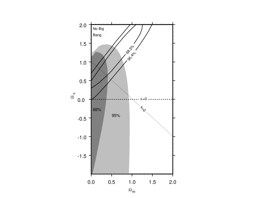
Figure 1: Two-dimensional constraints obtained using radio galaxies (shaded regions) compared with those from obtained by the supernovae cosmology team using supernovae (solid lines)(see Perlmutter et al. 1999 and GDW00). One-dimensional constraints obtained using radio galaxies are discussed in the text.

Figure 2: Two-dimensional constraints obtained using radio galaxies (shaded regions) compared with those obtained by the high-redshift supernovae team using supernovae (solid lines) (see Riess et al. 1998 and GDW00). One-dimensional constraints obtained using radio galaxies are discussed in the text.

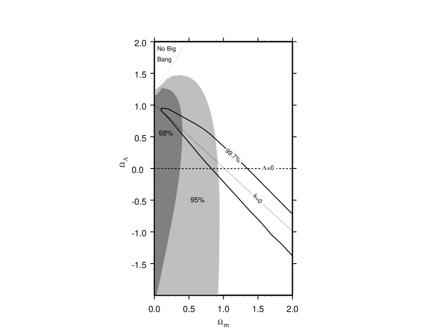
Figure 3: Two-dimensional constraints from radio galaxies (shaded regions) compared with those from CMB anisotropy (solid lines) (see Bond et al. 2000 and GDW00). The CMB anisotropy measurements indicate that k = 0.

The radio galaxy method uses FRIIb radio galaxies as a modified standard yardstick, and is described in more detail in section 3. The method relies on a comparison between an individual source and the properties of the parent population at the source redshift. The radio surface brightness and width of the radio source can be used to predict the maximum source size, measured using the largest angular size of the source or the separation between the radio hotspots. The average source size $D_{*}$ is just half of the maximum source size predicted using the model. This determination of the average source length does not depend on the observed length of the source, $D$, and depends on the coordinate distance to the $(-2\beta/3)+(4/7)$ power: $D_{*}\propto(a_{o}r)^{(-2\beta/3)+(4/7)}$. The predicted average size of a given source is equated to the average size of all FRIIb radio galaxies at similar redshift $<D>$, and, of course, $<D>\propto(a_{o}r)$. Clearly the two measures of the average source size must be equal, or their ratio must be a constant, independent of redshift: $<D>/D_{*}=$ constant. And, their ratio depends on $(a_{o}r)^{(2\beta/3)+(3/7)}$. Thus, this method allows a determination of the model parameter $\beta$ and global cosmological parameters. It turns out that $\beta$ is relevant to models of jet formation and energy extraction from AGN, as discussed in section 5, and by Daly & Guerra (2001b) [DG01b].

The radio galaxy and supernova methods are complementary, as shown in Table 1. They have a similar dependence on the coordinate distance; the power listed for radio galaxies is for a value of $\beta$ of 1.75, but this power does not change by very much given the range of $\beta$ allowed by the data ($\beta=1.75\pm 0.25$). They cover similar redshift ranges, though the radio galaxy method does go to redshifts of two. They have a similar number of sources, though the supernova method does have more sources than the radio galaxy method, and thus is much more well tested empirically, as noted in the table. The supernova method relies on a relation that is derived empirically, while the radio galaxy method relies on a relation that is derived using physical and theoretical arguments (see section 3). The supernova method is normalized at zero redshift, and depends quite strongly on the local distance scale and properties of local supernova. The radio galaxy method is not normalized at zero redshift, is completely independent of the local distance scale, and is independent of the properties of local sources. GDW00 show that the analysis can be carried using sources with redshifts greater than 0.3 only, and the results are identical to those obtained including sources with redshifts less than 0.3; this is also shown here in figures 4, 5, and 8. The radio galaxy method indicates that $\Omega_{m}$ must be low irrespective of the properties of the unknown component at zero redshift. This method also implies that if space curvature is zero, then it is quite likely (84 % confidence) that the universe is accelerating at the present epoch (see figure 9). The supernova method indicates that the universe is accelerating at the present epoch. The supernova method is well-tested empirically, but needs more theoretical understanding, while the radio galaxy method is better understood theoretically, and needs more empirical testing.

The supernova method relies on relatively short-lived optical events on the scale of stars, while the radio galaxy method relies on much more long-lived radio events on scales larger than the scale of galaxies. Thus, any possible selection effects or unknown systematic errors must be completely different for the two methods. The fact that they yield such similar results suggests that both are accurate, and are not plagued by unidentified errors.

The two-dimensional results obtained using radio galaxies are compared with those obtained using supernova and the cosmic microwave background allowing for space curvature, a cosmological constant, and non-relativistic matter, and are shown in figures 1, 2, and 3. Note, that the contours shown are a joint probability, so constraints on cosmological parameters can not be read directly from these figures. To read off constraints on individual cosmological parameters directly from a figure, the one-dimensional figure must be considered. For the radio galaxy method, these are presented in figures 4 and 5, and in GDW00 and DG01a. The radio galaxy sample includes 20 FRIIb galaxies for which $D_{*}$ has been computed, and the 70 FRIIb radio galaxies in the parent population. The 20 sources for which $D_{*}$ has been determined are a subset of the 70 sources that make up the parent population.

The fact that the methods constrain different parts of the $\Omega_{m}$-$\Omega_{\Lambda}$ plane is related to the fact that the methods cover different redshift ranges (e.g. Reiss 2000). Most of the supernovae data points are at redshifts less than about 1 or so. The radio galaxies are primarily at redshifts from 0.5 to 2, and the cosmic microwave background is at a redshift of about a thousand. Thus, the three data sets are complementary in their redshift coverage, and the constraints they impose.

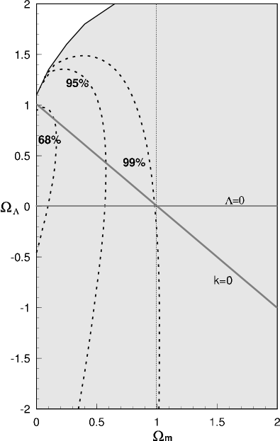
Figure 4: Constraint obtained using FRIIb radio galaxies. The projections of the 68%, 95%, and 99% confidence intervals onto either axis ($\Omega_{m}$ or $\Omega_{\Lambda}$) indicates the probability associated with the range in that one parameter, independent of all other parameter choices. That is, these are the one-dimensional confidence contours (see GDW00).

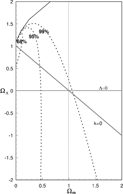
Figure 5: The same as Figure 4, excluding the lowest redshift bin (i.e. Cygnus A), from the fit. Only sources with redshifts greater than 0.3 are included in this analysis (see GDW00). The results are nearly identical to those presented in figure 4.

3 FRIIb Radio Galaxies as a Modified Standard Yardstick

A detailed description of FRIIb radio galaxies as a tool to determine global cosmological parameters may be found in Daly (1994), Guerra (1997), Guerra & Daly (1998), GDW00, DG01a,b.

FRIIb radio galaxies have very regular bridge structure. They are the most powerful FRII sources, having radio powers about a factor of 10 above the classical FRI-FRII separation. The regular bridge structure indicates that both the instantaneous and time-average rate of growth of the source is supersonic (e.g. Daly 2001).

The method is based on the following premises and assumptions: the forward region of FRIIb radio galaxies are governed by strong shock physics; the total source lifetime $t_{*}$ is related to the beam power $L_{j}$ via the relation $t_{*}\propto L_{j}^{-\beta/3}$; and the sources in the parent population at a given redshift have a similar maximum or average size. If these conditions are satisfied, then FRIIb radio galaxies provide a reliable probe of global cosmological parameters. Observations of FRIIb sources indicate that the forward region (near the radio hotspot) are governed by strong shock physics. A power-law relation between the beam power and the source lifetime is expected/predicted in currently popular models to produce large scale jets (DG01b). And, the dispersion in source size at a given redshift for the parent population of sources suggests that the sources at a given redshift do have a similar average size (see figure 6).

From these simple assumptions, the average size a given source will have if it could be observed over its entire lifetime is

$$D_{*}\propto(P_{L}a_{L}^{2})^{-\beta/3}~{}v_{L}^{1-\beta/3}\propto(a_{o}r)^{-2\beta/3+4/7}~{},$$ (1)

where each contributor to $D_{*}$ can be determined from radio bridge observations including the lobe pressure $P_{L}$, the lobe width $a_{L}$, and the average rate at which the bridge is lengthening $v_{L}$.

Minumum energy conditions are not assumed to hold in the bridges of the sources; an offset from minimum energy conditions is included, and is one of the parameters that is obtained from the analysis (see Wellman, Daly, & Wan 1997b [WDW97b]).

Figure 6: The average lobe-lobe size $\langle D\rangle$ of powerful extended 3CR radio galaxies for the 70 FRIIb radio galaxies that comprise the parent population of radio galaxies. Different choices of cosmological parameters are shown (here $\Omega_{m}=\Omega_{o}$). Note that $<D>\propto(a_{o}r)$.

Figure 7: The model dependent, average size $D_{*}$ the source would have if it could be observed over its entire lifetime computed assuming $\beta=1.75$, $b=0.25$, $\Omega_{m}=0.1$, and $\Omega_{\Lambda}=0$; b is the offset of the bridge magnetic field strength from the minimum energy value. Note that $D_{*}\propto(a_{o}r)^{-0.6}$.

The average size of a given source $D_{*}$ is assumed to be equal to the average size of the parent population at the same redshift $<D>$, where $<D>\propto(a_{o}r)$. Thus, the ratio $<D>/D_{*}$, which must be a constant, can be used to determine the coordinate distance to the source since

$$<D>/D_{*}\propto(a_{o}r)^{2\beta/3+3/7}~{}.$$ (2)

Figure 6 shows $<D>$ as a function of redshift, and figure 7 shows $D_{*}$ as a function of redshift. The method relies on the fact that $D_{*}\propto(a_{o}r)^{-0.6}$ for $\beta=1.75$, while $<D>\propto(a_{o}r)$. Thus, the method boils down to finding the cosmological parameters such that the shapes of the best-fitting curves to $D_{*}(z)$ and $<D>(z)$ match. That is why the method is independent of the local distance scale and of local sources. Differences between cosmological models begin to be obvious at redshifts greater than about 0.5; As shown in figure 6, the slope of the line that describes $<D>(z)$ steepens as the cosmological paramaters move from being dominated by a cosmological constant to an open universe to a matter-dominated $\Omega_{m}=1$ universe; this arises because $<D>\propto(a_{o}r)$. However, the slope of the line that describes $D_{*}(z)$ begins at its steepest and becomes less steep as the cosmological paramaters move from being dominated by a cosmological constant to an open universe to a matter-dominated $\Omega_{m}=1$ universe; this arises because $<D>\propto(a_{o}r)^{-0.6}$. Thus, the power of the method lies in the fact that only for the correct choice of cosmological parameters will the shapes of $D_{*}(z)$ and $<D>(z)$ be the same. The normalization of the fits is allowed to float; that is $<D>/D_{*}$ = constant, and the constant is an output of the fit.

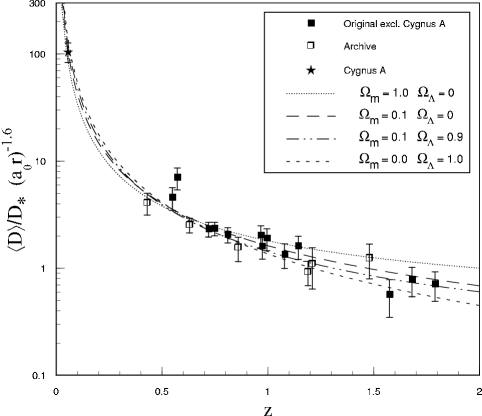
Figure 8: The quantity $(\langle D\rangle/D_{*})(a_{o}r)^{-1.6}$, computed assuming $\beta=1.75$ and $b=0.25$, where b parameterizes the offset from minimum energy conditions. Best fit models for different choices of $\Omega_{m}$ and $\Omega_{\Lambda}$ are shown, where sources with redshifts less than 0.3 have been excluded from the fits. Note that the fits are not normalized using local or low-redshift sources, yet all of the fits go right through the low-redshift point at a redshift of about 0.06 (Cygnus A) and $<D>/D_{*}(a_{o}r)^{-1.6}\sim 100$. The normalization is allowed to float for each fit.

The ratio of $<D>/D_{*}$ is shown in figure 8, where the ratio is multiplied by $(a_{o}r)^{-1.6}$ to remove the dependence of the ratio on cosmological parameters; a value of $\beta=1.75$ was adopted for illustrative purposes. The fits shown are obtained using only radio data with redshifts greater than 0.3, thus, this is independent of the local distance scale and the properties of local sources. The best fitting lines pass right through the data point at a redshift of about 0.06 (Cygnus A) and $<D>/D_{*}(a_{o}r)^{-1.6}=100$, which shows that the method is working quite well.

Evolution of source properties with redshift are much less of a concern for the radio galaxy method than for methods that rely upon the properties of local sources because the method relies on a comparison of individual source properties with the properties of the parent population.

4 Quintessence in a Spatially Flat Universe

The application of FRIIb radio galaxies to constrain the current value of the normalized mean mass-energy density $\Omega_{Q}$ and (time-independent) equation of state $w=P/\rho$ of quintessence in a spatially flat universe, $\Omega_{Q}=1-\Omega_{m}$, is presented by DG01a,b. The results are summarized here.

A universe with two primary components at the present epoch (non-relativistic matter and quintessence) will be accelerating in its expansion when

$$1+3w(1-\Omega_{m})<0~{}$$ (3)

(DG01a).

Figure 9 shows the one-dimensional constraints obtained using a sample of 20 FRIIb radio galaxies, which are a subset of the 70 FRIIb radio galaxies in the parent population. Most of the sources in the sample have redshifts between 0.5 and 2, and identical results obtain with and without the lowest redshift bin; again, the method is independent of the local distance scale and of the properties of local sources. Clearly, FRIIb radio galaxies indicate that the universe is likely to be accelerating in its expansion at the present time; this is about a 2 $\sigma$ result.

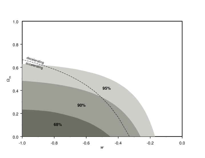
Figure 9: One-dimensional constraints on $\Omega_{m}$ and $w$ obtained using $D_{*}$ for 20 FRIIb radio galaxies, and assuming zero space curvature (see DG01a).

In any method, it is important to consider any possible covariance between constraints placed on different sets of parameters. For the FRIIb radio galaxy method, it is important to determine if there is any covariance between the global cosmological parameter $\Omega_{m}$ and the model parameter $\beta$. Figure 10 shows that there is no covariance between these parameters.

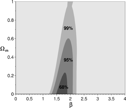
Figure 10: One-dimensional constraints on $\Omega_{m}$ and $\beta$ for quintessence models, assuming zero space curvture (see DG01a).

It is also important to insure that there is no covariance between the equation of state of quintessence $w$ and the model parameter $\beta$. Figure 11 shows that there is no covariance between these parameters.

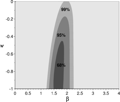
Figure 11: One-dimensional constraints on $w$ and $\beta$ for quintessence models, assuming zero space curvature (see DG01a).

Clearly, a cosmological constant, which has $w=-1$, is consistent with the data.

FRIIb radio galaxies can also be used to constrain global cosmological parameters allowing for space curvature, non-relativistic matter, and a cosmological constant (GDW00). The results indicate that $\Omega_{m}$ must be less than one, and $\Omega_{m}=1$ is ruled out at about 99 % confidence. Figures 12 and 13 show that there is no covariance between the model parameter $\beta$ and the cosmological parameter $\Omega_{m}$ allowing for a cosmological constant, or space curvature.

Figure 12: One-dimensional constraints on $\Omega_{m}$ and $\beta$ assuming zero space curvature and allowing for a cosmological constant (see GDW00).

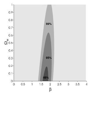
Figure 13: One-dimensinal constraints on $\Omega_{m}$ and $\beta$ assuming no cosmological constant and allowing for space curvature (see GDW00).

5 Implications for the Beam Power - Total Energy Connection

Studies of FRIIb radio galaxies indicate that the total time $t_{*}$ for which the central black hole produces collimated jets with beam power $L_{j}$ that ultimately power the strong shocks near the hotspots and lobes of a given source are described by

$$t_{*}\propto L_{j}^{-\beta/3}~{}.$$ (4)

The total energy $E_{*}=L_{j}t_{*}\propto L_{j}^{1-\beta/3}$, and the beam power is related to the total energy available to power the outflow

$$L_{j}\propto E_{*}^{3/(3-\beta)}~{}.$$ (5)

Thus, $L_{j}\propto E_{*}^{2~{}to~{}3}$ for $\beta=1.5$ to 2; recall that $\beta=1.75\pm 0.25$.

An analysis of the implications for models of jet production is given by DG01b, and is briefly summarized here. If the jets are powered by the electromagnetic extraction of the rotational energy of a spinning black hole (Blandford 1990), then equation 4 and 5 implies that the magnetic field $B$ must be related to the black hole mass $M$, the spin angular momentum $S$ per unit mass $a=S/(Mc)$, and the effective size of the black hole $m=GM/c^{2}$, via the relation

$$B\propto M^{(2\beta-3)/2(3-\beta)}(a/m)^{\beta/(3-\beta)}~{},$$ (6)

as detailed by DG01b. Equation 6 takes a particularly simple form for $\beta=1.5$; in this case, $B\propto(a/m)$. For a value of $\beta$ of 1.75, equation 6 implies that $B\propto M^{0.2}(a/m)^{1.4}$, and for $\beta=2$, $B\propto M^{1/2}(a/m)^{2}$. Specific values for B, $L_{j}$, and $E_{*}$ are described below, where this model is discussed further.

If the jets are powered by radiation that is Eddington limited so $L_{j}=\eta_{L}L_{E}\propto\eta_{L}M$, where $L_{E}$ is the Eddington luminosity, $\eta_{L}$ is the efficiency with which the radiant luminosity is converted into beam power, $M$ is the black hole mass, and the accreted mass $M_{acc}$ is converted to energy with an efficiency $\eta_{E}$ so that $E_{*}=\eta_{E}M_{acc}c^{2}$ (e.g., Krolik 1999), then equation 5 implies that

$$\eta_{L}\propto\eta_{E}^{3/(3-\beta)}(M/M_{acc})^{-3/(3-\beta)}M^{\beta/(3-\beta)}~{}.$$ (7)

For $\beta=1.5$, this reduces to $\eta_{L}\propto\eta_{E}^{2}(M/M_{acc})^{-2}M$. The beam power could be as high as the Eddington luminosity, or could be a constant fraction of the Eddington luminosity, in which case

$$\eta_{E}\propto(M/M_{acc})M^{-\beta/3}~{},$$ (8)

or $\eta_{E}\propto M^{-1/2}$ for $\beta=1.5$ and $M_{acc}\sim M$.

The total energy that will be processed by each source through each of its two large-scale jets over its lifetime $E_{*}$ is shown as a function of core-hotspot separation in Figure 14 and as a function of redshift in Figure 15.

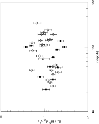
Figure 14: The total energy processed through each beam of each source as a function of core-hotspot separation; open symbols represent the 14 radio galaxies in the original sample (see GD98), and the filled symbols represent the 6 radio galaxies obtained from the VLA archive (see GDW00). Most sources have 2 data points, one from each side of the source.

Figure 15: The total energy processed through each jet of each source as a function of redshift. The symbols are the same as in figure 14.

The beam powers of the sources are shown in Figure 16 as a function of core-hotspot separation, and in Figure 17 as a function of redshift.

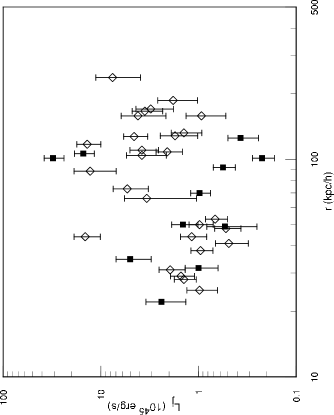
Figure 16: The beam power processed through each side of each source as a function of core-hotspot separation. The symbols are the same as in figure 14.

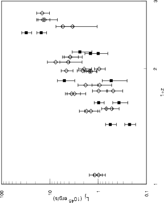
Figure 17: The beam power processed through each side of each source as a function of redshift. The symbols are the same as in figure 14.

Clearly, the beam power increases with redshift. However, if the beam power is related to the Eddington luminosity, then it is proportional to the black hole mass, which is expected to increase with time, or decrease with redshift. In addition, the beam powers are typically about $10^{45}$ erg/s, implying a black hole mass of only about $10^{7}M_{\odot}$, which is smaller than the black hole masses associated with galaxies in the cores of clusters of galaxies. The scaling of the beam power, total energy, and total source lifetime as given above, and can be normalized using the fact that when the beam power is $L_{j}\sim 10^{45}erg/s$, the total active lifetime is $t_{*}\sim 10^{7}$ yr, and the total energy processed through the jet is $\sim 5\times 10^{5}c^{2}M_{\odot}$ (see DG01b, or figures 14, 16, and 18).

Since the sources seem to be preferentially located near the cores of clusters or protoclusters of galaxies (see Wellman, Daly, & Wan 1997a [WDW97a] and WDW97b), a model in which a massive black hole acquires substantial rotational energy after coallescing with another massive black hole, such as that of Wilson & Colbert (1995) is quite attractive. A timescale can be constructed by dividing $E_{*}$ by $L_{EM}$; using equations (3.38) and (3.39) from Blandford (1990), the timescale of the outflow is of order $10^{9}/(M_{8}B_{4}^{2})$ yr, where $M_{8}$ is the mass of the black hole in units of $10^{8}M_{\odot}$, and $B_{4}$ is the magnetic field strength in units of $10^{4}$ G. A total lifetime of about $10^{7}$ yr results for a black hole mass of about $10^{9}M_{\odot}$ and a field strength of about $3\times 10^{4}$ G. These values would lead to beam powers of about $10^{45}$ erg/s and total energies of about $10^{60}$ erg, equivalent to a rest mass of about $5\times 10^{5}M_{\odot}$, for $(a/m)\sim 1/30$, which are reasonable numbers, and which agree with the results obtained empirically.

For comparison, the total lifetimes of the 20 sources studied here are shown in figure 18 as a function of core-hotspot separation, and in figure 19 as a function of redshift. Clearly, high-redshift sources have shorter total lifetimes.

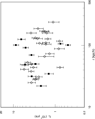
Figure 18: The total jet lifetime for each side of each source as a function of core-hotspot separation. The symbols are the same as in figure 14.

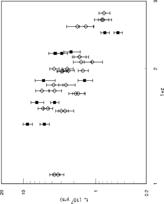
Figure 19: The total jet lifetime for each side of each source as a function of redshift. The symbols are the same as in figure 14.

6 FRIIb Radio Sources Provide Probes of Evolution of Structure

The structure of the radio bridges of FRIIb sources can be used to determine the ambient gas pressure, density, temperature, and the overall Mach number of the forward region of the source, as detailed in a series of papers (Wan & Daly 1998; WDW97a,b; WDG00). The use of the properties of the radio bridge to determine the ambient gas pressure does not rely upon the assumption of minimum energy conditions, and it is independent of the rate of growth, or lobe propagation velocity, of the source, and hence is independent of any aging analysis applied to the radio bridge. The sources are in gaseous environments with pressures and composite pressure profiles like those found in clusters of galaxies, though some redshift evolution of the ambient gas pressure is suggested by the results obtained.

The ambient gas density may be obtained by studying the ram pressure confinement of the forward region of the radio source. This is done by combining the rate of growth of the source, determined using a spectal aging analysis across the radio bridge of the source, with the pressure near the end of the source, as done by Perley & Taylor (1990) for 3C295, Carilli et al. (1990) for Cygnus A, WDW97a for a sample of 14 radio galaxies and 8 radio loud quasars, and GDW00 for a sample of 6 radio galaxies. These studies indicate that the sources are in cluster-like gaseous environments, though some redshift evolution of the density and density profile is indicated by the study of WDW97b.

The shape of the radio bridge leads to a determination of the average Mach number with which the forward region of the source moves into the ambient gas (WDW97a). The Mach number can be combined with the rate of growth of the source, or lobe propagation velocity, to obtain the temperature of the ambient gas (WDW97a). This analysis also indicates that the sources are in gaseous environments with temperatures similar to those in present day cluster of galaxies.

Thus, there are some indications from the properties of FRIIb radio sources that they are in the cores of clusters or proto-clusters of galaxies, and that the properties of the gas in the cores of galaxy clusters evolves from a redshift of zero to a redshift of two.

7 Conclusions

FRIIb radio galaxies provide a probe of the coordinate distance to very high redshift sources, including sources with redshifts between one and two. The results obtained using FRIIb radio galaxies are consistent with those indicated by measurements of the cosmic microwave background (de Bernardis et al. 2000, Balbi et al. 2000, Bond et al. 2000), and type Ia supernovae (Riess et al. 1998, Perlmutter et al. 1999). The modified standard yardstick method, which uses FRIIb radio galaxies, is complementary to the modified standard candle method, which uses type Ia supernovae. Possible sources of error in each method are likely to be very different. Thus, the fact that they yield consistent results suggests that any errors not yet accounted for in either method must be small compared with errors that are currently known and accounted for.

FRIIb radio galaxies indicate that $\Omega_{m}$ must be low; $\Omega_{m}=1$ is ruled out at about 99 % confidence. Measurements of the cosmic microwave background radiation indicate that the universe has zero space curvature (e.g., Bond et al. 2000). In a universe with zero space curvature and quintessence with equation of state $w$, the modified standard yardstick method using FRIIb radio galaxies indicates that it is likely that the expansion of the universe is accelerating at present. The expansion rate of the universe will be accelerating when

$$1+3w(1-\Omega_{m})<0~{},$$ (9)

DG01a. This line is drawn on Figure 9; the region below the line indicates that the universe is accelerating at present; those above the line indicate a decelerating universe. Radio galaxies alone indicate that the universe is accelerating in its expansion at the current epoch; this is an 84 % confidence result.

The application of the modified standard yardstick method not only allows a determination of global cosmological parameters, it also allows a determination of the model parameter $\beta$; current results indicate that $\beta$ is about $1.75\pm 0.25$. The parameter $\beta$ can be used to constrain models of energy extraction from the central massive object, presumed to be a massive black hole; these constraints are described by DG01b and are summarized in section 5. The value of $\beta$ determined empirically is expected/predicted in models where jet formation, power, and energy are related to the electromagnetic extraction of the rotational energy of a spinning black hole, and is consistent with models in which jet production is related to the Eddington luminosity of the black hole region.

Independent of the application of FRIIb radio galaxies to constrain cosmological parameters and models of energy extraction from massive black holes, FRIIb radio galaxies can also be used to study the gaseous environments of this type of AGN. The sources may be used to study the pressure, density, and temperature of the gas around them, and appear to be located in the cores of clusters or protoclusters of galaxies, as summarized in section 6.

FRIIb radio sources appear to be governed by strong shock physics, and hence are in a regime that is easy to quantify. This fact, coupled with the interesting relation between the beam power and total energy that all of the sources seem to follow, makes them ideally suited to cosmological studies. In addition to their use as a modified standard yardstick, they also provide a probe of models of evolution of structure through their use to study the properties of the cores of clusters or proto-clusters of galaxies. The fact that they are located near the centers of clusters or proto-clusters of galaxies is probably related to the similar physical mechanism of jet formation and energy extraction.