Tree-Structured Grid Model of Line and Polarization Variability from Massive Binaries

We have developed a 3-D Monte Carlo radiative transfer model which computes line and continuum polarization variability for a binary system with an optically thick non-axisymmetric envelope. This allows us to investigate the complex (phase-locked) line and continuum polarization variability features displayed by many massive binaries: W-R+O, O+O, etc. An 8-way tree data structure constructed via a “cell-splitting” method allows for high precision with efficient use of computer resources. The model is not restricted to binary systems; it can easily be adapted to a system with an arbitrary density distribution and large density gradients. As an application to a real system, the phase dependent Stokes parameters $\left(I,\,Q,\,U\right)$ and the phase dependent He i ($\lambda$5876) profiles of the massive binary system V444~Cyg (WN5+O6 III-V) are computed.

1 Introduction

Linear polarization of light is often used to study the geometrical distribution of gaseous/dusty materials around various types of astronomical objects, e.g., close binaries, Be stars, Wolf-Rayet (W-R) stars, Luminous Blue Variables (LBVs), supernovae, Seyfert galaxies, quasars (QSOs), and Young Stellar Objects (YSOs). When the angular size of an object is too small to be resolved by ground-based or space telescopes, spectropolarimetry and narrow band polarimetry provide useful information on the geometry of circumstellar matter.

Several analytic models use simplifying assumptions to predict the continuum polarization levels arising from electron scattering envelopes. For example, Brown & McLean (1977) derived an expression for the degree of polarization produced in an optically thin axisymmetric envelope with an embedded point source. Brown et al. (1978) extended this model, deriving the expressions for the polarization arising from a binary system embedded in an optically thin envelope. Adopting this model, Brown et al. (1989) considered the effect of the finite size of the light source. Unfortunately, these 2-D models lack an ability to investigate more complex systems such as close binaries with colliding stellar winds, molecular clouds with fractal structure, and the tails of non-circular accretion flows. Further, they can not deal with the realistic inhomogeneities present in many scattering envelopes, and they are not suitable for optically thick atmospheres with multiple scattering.

In order to investigate such complicated systems, we abandon the simplifying assumptions and use a full three dimensional model that can handle an optically thick atmosphere. Formulating and solving the radiative transfer equation for an arbitrary geometry is difficult even for continuum radiation. The presence of additional scattering integrals in the expression for the source function and the need to solve several coupled transfer equations for the Stokes parameters tremendously complicates the problem. The flexibility of Monte Carlo methods of radiative transfer are particularly useful for such problems despite the fact that they may not be the most efficient solution method. For example, asymmetries in the radiation field, non-spherical geometry, and a complex distribution of the clumps can be readily incorporated. The issue of efficiency is less severe due to the significant advancement of computer technology. In the near future, it may be possible to perform non-LTE radiative transfer calculations in 3-D including thousands of lines from multi-atomic species utilizing some of the ideas described by Bernes (1979) and Li & McCray (1996). Recently, Lucy (1999) developed an improved Monte Carlo technique for non-LTE radiative transfer calculations applied to a synthetic supernova spectra model.

Our main reason for developing a 3-D model is to investigate the colliding wind (CW) interaction zone. Such zones are relatively common among massive binaries (W-R+O, O+O binaries). Koenigsberger & Auer (1985) found, using low resolution IUE spectra, that 3 out of 6 selected W-R+O binaries showed evidence for CWs. Shore & Brown (1988), Marchenko et al. (1994) and Marchenko et al. (1997) presented detailed studies of CW related variability seen in high-resolution UV and optical data of V444~Cyg (WN5+O6 III-V). Stevens & Howarth (1999) presented observations of the phase dependent He i (1.0830-$\mu$m) line profile in six different W-R binary systems including V444~Cyg. Using a simple model, they explained the observed variability in terms of the wind-wind interaction. Further theoretical aspects of the relationship between X-ray variability and CWs have been developed by Luo et al. (1990) and Stevens et al. (1992). More recently, detailed hydrodynamic models of colliding winds have be used by Stevens & Pollock (1994), Gayley et al. (1997) and Pittard (1998). Simulations of the colliding winds in V444~Cyg are given in Pittard & Stevens (1999).

Examples of 3-D Monte Carlo radiative transfer models recently developed are Witt & Gordon (1996), Pagani (1998), Stevens & Howarth (1999), Wolf et al. (1999) and Harries (2000). Juvela (1997) presented their 1-3 dimensional Monte Carlo models of emission from clumpy molecular clouds. Wolf et al. (1999) developed a self-consistent 3-D continuum Monte Carlo model in which the dust temperature and the radiation field are iterated to consistency. These 3-D models, with the exceptions of Wolf et al. (1999) and Harries (2000), use regular “cubic” grids and are not suitable for a model with a large density gradient or a large dynamic range of density. These would require much finer grid sizes (and hence more memory) to resolve the smaller structures. Wolf et al. (1999) and Harries (2000) used 3-D grids in spherical coordinates. Their grids are evenly spaced in polar and azimuthal angles, but logarithmically spaced in the radial direction. This type of grid is useful for a system that does not deviate much from spherical or axisymmetric symmetry, but it would not be adequate for a binary system with colliding stellar winds or for a binary system with accretion flow from a companion.

Starting from the 2-D Monte Carlo model of Hillier (1991), we have developed a 3-D Monte Carlo code to calculate the continuum and line polarizations produced by the scattering of light in an arbitrary geometry. The model can predict the variability features associated with the orbital motion of a binary system, such as the polarization level, flux level, and line profile shapes. The model can treat a finite size stellar disk, multiple scattering, absorption of continuum photons by a line, and emission from multiple light sources (extended or not). Higher precision is achieved with fewer grid points by using a “cell-splitting” method whose application to this type of problem was discussed by Wolf et al. (1999). We extended the idea of “cell-splitting” to a simple 8-way tree data structure to construct the model grids. With this data structure, we can quickly access the data stored at any grid point, leading to a faster, more efficient, numerical code. This is essential to our model because of the high dimensionality and because no assumptions are made regarding the symmetry of the model. A logarithmic grid, like those commonly used in spherical and axisymmetric codes, is not readily implementable.

In § 2, we describe the details of our model. Various accuracy and efficiency tests are given in § 3. The model is applied to the massive binary V444~Cyg (WN5+O6) as an example calculation for a real system in § 4. The conclusions are given in § 5.

2 Model

2.1 Polarization

A general method of polarization calculation via the Monte Carlo method is described in Modali et al. (1972), Sandford (1973), Warren-Smith (1983) and Hillier (1991). An initial photon beam emitted from a light source is usually assumed to be unpolarized, with the Stokes parameters given by $(I,Q,U,V)=(I_{o},0,0,0)$. After each scattering, the Stokes parameters change according to the Mueller matrix, $M(\theta,\phi)$ where $\theta$ and $\phi$ are the polar and azimuthal scattering angles respectively.

$$\left(\begin{array}[]{c}I^{\prime}\\ Q^{\prime}\\ U^{\prime}\\ V^{\prime}\end{array}\right)\propto M(\theta,\phi)\left(\begin{array}[]{c}I\\ Q\\ U\\ V\end{array}\right)$$

In the case of Thomson scattering , $M$ has no $\phi$ dependency, and it becomes

$$M=\left(\begin{array}[]{cccc}\frac{1}{2}(1+\mu^{2})&-\frac{1}{2}(1-\mu^{2})&0&0\\ -\frac{1}{2}(1-\mu^{2})&\frac{1}{2}(1+\mu^{2})&0&0\\ 0&0&\mu&0\\ 0&0&0&\mu\end{array}\right)$$

where $\mu=\cos\theta$.

A coordinate transformation of the Stokes parameter vector $\Lambda^{T}=\left(I,Q,U,V\right)$ to a fixed reference frame is necessary after each scattering. Chandrasekhar (1960) describes how this transformation is done. After several scattering events, the photon beam will reach the model boundary (cubic in our case), and the $\Lambda^{T}$ vector will then be projected onto the plane of an observer. The reader is refer to Hillier (1991) for details.

2.2 Coordinates

For the model discussed here, we assume that the density distribution is co-rotating with the binary system, and the orbit is circular. Two coordinate systems are used in the model (see Fig. 1). One is the primary star coordinates (x, y, z), and the other is the binary coordinates (x’, y’, z’). The binary coordinate system is a rotating coordinate system, and it is chosen such that the stars and the density are fixed (or independent of orbital phases) in that coordinate system. The orbital plane is assigned to be on the x-y plane of the primary star coordinates. The primary star (Star A) is placed at the origin of the two coordinate systems, and the secondary star (Star B) is placed on the x’ axis. The relative position of two coordinate systems changes as a function of orbital phase ($t$). When $t=0$, the two coordinate systems coincide. For $t>0$, the primed (binary) coordinate system rotates around the z axis of the unprimed (primary star) coordinates making the angle between x & x’ and y & y’ to be $\Theta\left(t\right)$. For a circular orbit the relative angle is simply, $\Theta\left(t\right)=2\pi\,t$. In general, the separation distance $a$ is a function of $t$, but for a circular orbit $a$ remains constant. By our convention, an observer is always on the y-z plane with an inclination angle $i$ measured from z or z’ axis.

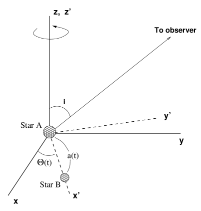
Figure 1: This illustrates the two coordinate systems used in the models. The binary coordinates (x’, y’ z’) rotates around the primary star coordinates (x, y, z) through the common z or z’ axis. A rotation angle ($\Theta$) and a binary separation ($a$) are functions of orbital phase $t$. For a circular orbit, they are simply, $\Theta\left(t\right)=2\pi$ and $a=$constant. An observer is placed on the y-z plane with the viewing angle $i$. The primary star (Star A) is placed at the origin of the two coordinate systems, and the secondary star (Star B) is placed on the x’ axis. With this configuration, the orbit of the binary is confined on x-y plane.

In the primary star (unprimed) coordinates, the locations of the stars, as a function of $t$, become

$$\left(\begin{array}[]{c}x_{A}(t)\\ y_{A}(t)\\ z_{A}(t)\end{array}\right)=\left(\begin{array}[]{c}0\\ 0\\ 0\end{array}\right)$$ (1)

and

$$\left(\begin{array}[]{c}x_{B}(t)\\ y_{B}(t)\\ z_{B}(t)\end{array}\right)=\left(\begin{array}[]{c}a\cos\left\{2\pi\left(t+t_{0}\right)\right\}\\ a\sin\left\{2\pi\left(t+t_{0}\right)\right\}\\ 0\end{array}\right)$$ (2)

where $2\pi t$ is the relative angle between the two coordinates and $t_{0}$ is an initial phase offset. In our model $t_{0}=-1/4$ is used so that when $t=0$, the secondary star (Star B) is behind the primary star (Star A) from an observer’s perspective. Eqs. 1 and 2 can be easily modified to an orbit with non-zero eccentricity for a general binary orbit.

2.3 Grid Selection

When the gradient in the opacity field is very large, a logarithmic scale in the radial direction can be used to increase computational accuracy of the optical depth if the system is spherically or axially symmetric. For the case of an arbitrary geometry, there is no simple way to construct a logarithmic scale. However, an efficient cubic grid (consisting of cubic cells) can be constructed by subdividing a cube into smaller cubes where the value of the opacity/emissivity is larger than a given threshold value. Wolf et al. (1999) introduced the basic idea for this type of grid method to the radiative transfer problem. We do not know the exact algorithm they used, but we have utilized the 8-way tree data structure to construct the grids and to store the values of the opacities. In addition to being conceptually simple, the advantages of using a tree data structure include increases in optical depth calculation accuracy, computer memory efficiency, and data access time. In the following subsections, we describe the algorithm for constructing the tree-structured grid and illustrate its efficiency.

2.4 Tree Data Structure Construction Algorithm

The data structure used here is similar to a “binary tree” in which one node splits into two children nodes, but ours splits into eight. The steps for the tree construction are summarized below. Fig. 2 gives the flow chart of the steps.

1. Start from a cubic box (root node) which holds the whole density structure.

2. Pick (100-1000) random locations, $\mathbf{r}=(x,y,z$), in the cell, and compute

   $$E=\frac{1}{n}\sum^{n}_{i=1}\eta_{i}^{p}\,d^{3}$$ (3)

   where $\eta_{i}$ is the emissivity at $i$-th random location, $n$ is the total number of the random locations, $d$ is the size of the cell and $p$ is the index of scalability.

3. If $E$ is greater than $E_{\mathrm{o}}$ which is a user specified parameter, divide the box into 8 equal-size cubes (child nodes). If $E$ is smaller than $E_{\mathrm{o}}$, do nothing.

4. For each cell just created, repeat Steps 2 and 3 until all cells have $E<E_{\mathrm{o}}$. — The lowest level cells are often called “leaf(s)” (leaves).

The index $p$ in Eq. 3 controls how fast the cell should be split with $\eta$, and normally $p=1$ is used. When $p=1$, $E$ represents the average “emission measure” of the cell since it simply becomes the product of the average emissivity and the volume of the cell. The emissivity at a given point can be evaluated from one or a combination of the following: 1. an analytical formula, 2. an interpolation of the output from a radiative transfer model and 3. an interpolation of the output from a hydrodynamical model. Other more complex algorithms could be used to optimize the computation for a specific problem.

Once the data structure is built, the access/search for a given cell can be done recursively, resulting a faster code. Examples of the resulting grids are shown in Fig. 3. The top diagram in Fig. 3 shows the grids constructed for two stars with different sizes having spherically distributed gas around each star. The figure clearly shows that the grid size becomes naturally smaller where the density is higher. The grids used for this density is in 3-D, but the diagram shows only the cross section of the y-z plane for clarity. In the bottom diagram of Fig. 3, the grids are overlaid with a pseudo-spiral galaxy density distribution (3-D but drawn in 2-D). The density of the disk is inversely proportional to the distance from the center of the galaxy except for the bulge region where the density is constant. The grids nicely follow the spiral arms, and become smaller as they approach to the center.

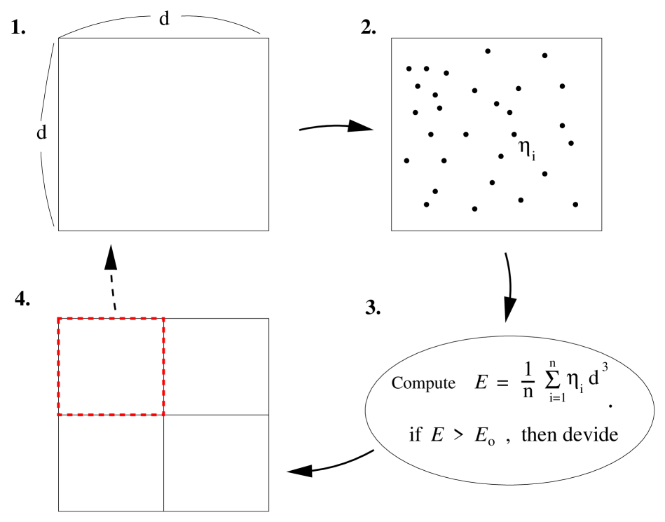
Figure 2: This diagram shows how a cell in a model space will be split into 8 subcells. 1. Consider a cubic cell with length “d.” 2. Choose n random locations in the cell, and evaluate the emissivity value $(\eta_{i})$ at each location. Average these emissivities to obtain $E$. 3. If $E$ is greater than a threshold value $E_{\mathrm{o}}$, then 4. Divide the cell into 8 equal size cubic cells. The program will repeat this procedure recursively until all the cells satisfy the condition: $E<E_{\mathrm{o}}$. Note that the figure shows the cell split into only 4 cells because the 3-D cell is projected onto a 2-D plane for clarity.

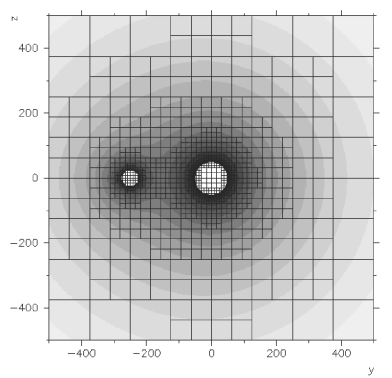
Figure 3: Examples of the tree structured grids. Top: a binary system with different stellar radii surrounded by a spherical atmosphere around each star. Bottom: a two-arm pseudo spiral galaxy. The density decreases as $\propto 1/r^{2}$ for $r>R_{b}$ and it is constant for a $r<R_{b}$ where $R_{b}$ is the bulge radius. Note that the real density distributions are 3-D, but here they are depicted in 2-D for simplicity. In both cases, the grid size naturally decreases for the high density regions.

2.5 Searching for a Cell

An example of how to find the cell which contains a point ($p$) in the tree data structure is illustrated in Fig. 4. The steps shown here are for the 2-D case for clarity, and the same method can be applied to the 3-D case. The figure shows the following steps:

1. Starting from the root cell (the outer most cell), outlined with a thick solid line, check whether the point is in the left half or the right half of the cell.

2. The point is in the right half of the cell; hence, dismiss all the subcells in the left half.

3. Further, check whether the point is in the upper half or the lower half of the cell outlined with a thick solid line. The point is in the upper half of the cell; hence, dismiss all the subcells in the lower half.

4. Further, check whether the point is in the left half or the right half of the cell outlined with a thick solid line.

5. The point is in the right half of the cell; hence, dismiss all the subcells in the left half. Further, check whether the point is in the upper or the lower of the cell outlined with a thick solid line.

6. The point is in the lower half of the cell. Since this is the lowest level (leaf node) of the tree, the search stops here. The leaf cell containing point $p$ is found.

In our algorithm, whether a point belongs to the left half or the right half of the cell and whether a point belongs to the upper half or the lower half of the cell are checked simultaneously. Therefore, steps 1 and 2 are considered to be just one step, as are steps 3 and 4. In other words, the total number of steps required to find the cell including point $p$ is considered to be “two” in this example.

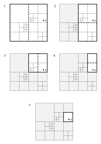
Figure 4: An illustration of how the cell which contains a point ($p$) in the model space can be found in the tree data structure. The figure demonstrates the searching steps for the 2-D case for clarity, but the same method can be applied to the 3-D case. The thick solid line indicates the cell that is focused in each step. The thick dotted lines represent the border used to check which side of the cell point p occupies. The corresponding instructions for each step are summarized in § 2.5.

2.6 Performance Check

To demonstrate the efficiency of the tree structure, the optical depth and the volume integral of density were computed with a (single-size) regular cubic grid and a tree structure grid separately. The functional forms of the opacity and the density used are $\chi\left(r\right)=\chi_{0}/r^{4}$ and $\rho\left(r\right)=\rho_{0}/r^{2}$ respectively. The top graph in Fig. 5 shows the percentage error of the optical depth calculations with the tree structure grid and that with one-size cubic grids as a function of “total” number of grid points. Similarly, the bottom graph in Fig. 5 shows the percentage error of volume integrals as a function of total number of grid points. Note that no special integration weights were used in both cases.

The figure shows the error decreases very quickly as the total number of grid/node points increases for the tree structure grids. As a consequence, much smaller number of points is required for the tree method to achieve the same order of accuracy, and thus the method requires much less computer memory. This enables us to do a realistic 3-D simulation even on a regular PC with a reasonable amount of RAM.

The number of steps in a grid searching routine depends on the complexities of the data structure, but in the case of the grids constructed with the inverse-square density function with the total grid points of $\sim 10^{6}$, the average number of searching steps is about 5. Although not implemented to the current model, the searching could be made more efficient by searching upward from the current position of a photon rather than searching downward from the root node each time since the cells along a photon trajectory are correlated.

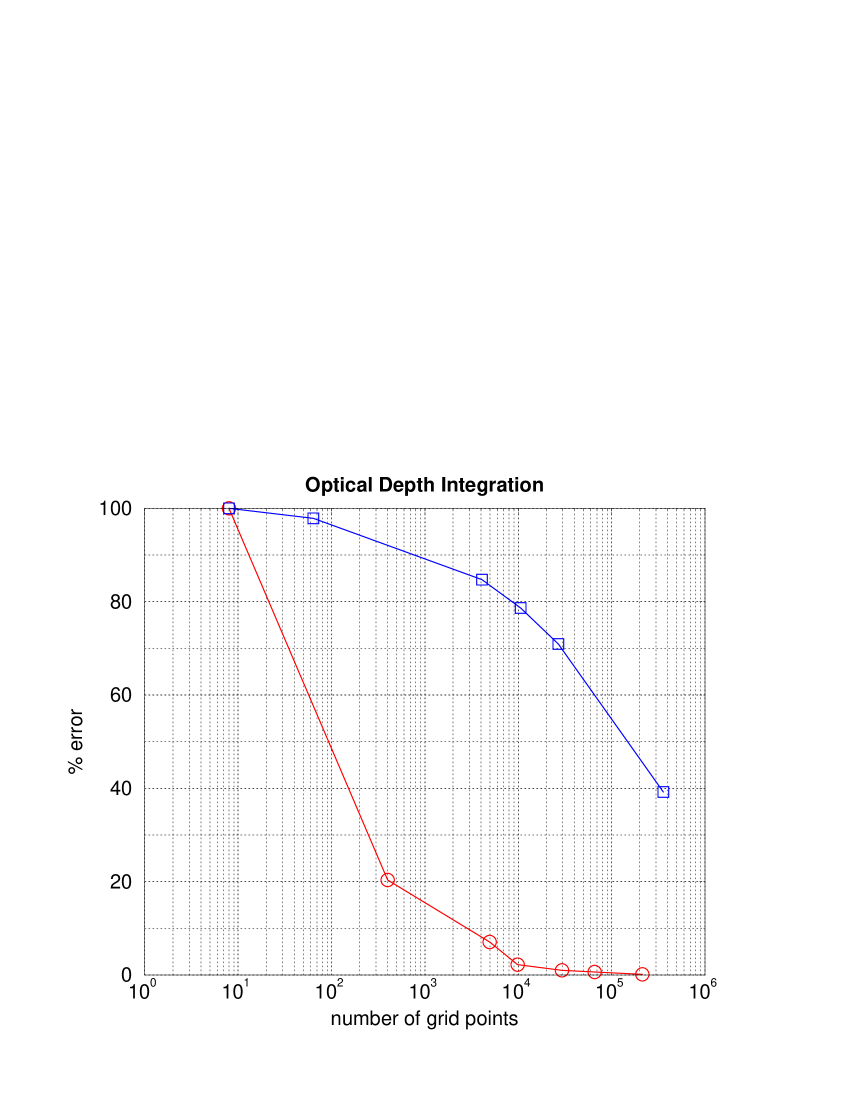
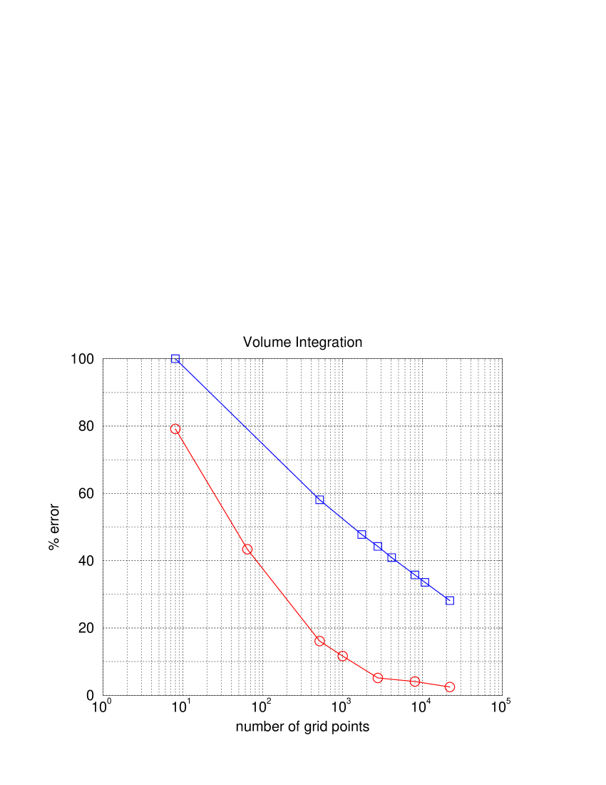
Figure 5: Top: Percentage errors of optical depth integrals using a regular grid (squares) and using a tree structured grid (circles) v.s. total number of grid points. The opacity is set to be $\chi=\chi_{0}/r^{4}$, and the optical depth is calculated from the surface of a star ($r=1R_{*}$) to the outer boundary of the model ($r=100R_{*}$). Bottom: Percentage errors of volume integrals $\left(\sum_{all\,cells}\rho_{i}dV_{i}\right)$ using a regular grid (squares) and using a tree structured grid (circles) v.s. total number of grid points. The density is assumed to be $\rho=\rho_{o}/r^{2}$, the integration limits are $r_{\mathrm{min}}=1R_{*}$ and $r_{\mathrm{max}}=100R_{*}$ where $R_{*}$ is the radius of a star.

2.7 Optical Depth

Suppose a photon at $\mathbf{r}_{o}=(x_{o,}y_{o},z_{o})$ is moving in the direction of $\mathbf{N}$ as shown in Fig. 6. This photon will most likely intersect with many cells (or grids) before it reaches the outer boundary. Calculation of the optical depth for a photon which is at $\mathbf{r}_{o}$ and moving in direction $\mathbf{N}$ is done by replacing the integral along the ray with the sum of the product of the cell opacity ($\chi_{i}$) with the line length ($\delta s_{i}$) of the photon beam in the cell, yielding

$$\tau=\int\chi(s)\,ds\approx\sum^{m}_{i=1}\chi_{i}\,\delta s_{i}$$ (4)

where $\chi_{i}$ is the sum of thermal and electron scattering opacities for a continuum photon:

$$\chi_{i}=\chi_{i}^{th}+\chi_{i}^{es}$$

and $m$ is the number of cells which intersect with the photon. In order to perform the summation in Eq. 4, we first need to find with which cells the photon will intersect. Then, the opacity values stored in these cells must be extracted. The location of the intersections on the cells must be found in order to calculate $\delta s_{i}$ in Eq. 4. As mentioned before, the searching for the intersecting cells and the values stored in the cells are relatively fast since the data is stored in the tree data structure.

Finding the intersections of a photon beam with model grids is relatively simple for a spherically symmetric system. In the tree grid case, the following must be done to find the intersecting points:

1. For all the planes of the cells which could have intersected with this photon, the following set of equations must be solved for $(x,y,z)$. The first one is the equation of the line along which the photon would move, and the second is the equation of the plane.

   $$\frac{(x-x_{0})}{N_{x}}=\frac{(y-y_{0})}{N_{y}}=\frac{(z-z_{0})}{N_{z}}$$ (5)

   $$(x-x_{c})\,n_{x}+(y-y_{c})\,n_{y}+(z-z_{c})\,n_{z}=0$$ (6)

   where $(x_{c},y_{c},z_{c})$ is a point on a face of the cube, $(x_{0},y_{0},z_{0})$ is the current location of photon, $\mathbf{n}=(n_{x},n_{y},n_{z})$ is the normal vector of a face, and $\mathbf{N}=(N_{x},N_{y},N_{z})$ is the directional vector of the photon.

2. There may be up to three such intersections (since the ranges of the coordinates are not restricted in Eqs. 5 and 6), but we are only interested in the first intersection which a photon encounters. The distance to each intersection must be calculated, and the smallest distance is used to compute $\delta s_{i}$ in Eq. 4.

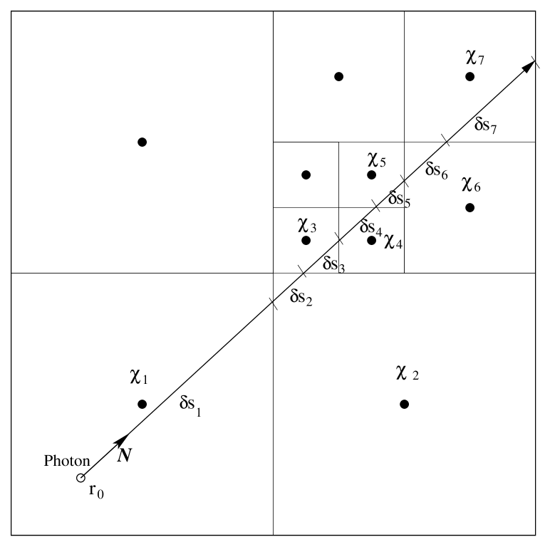
Figure 6: This diagram shows a photon at $\mathbf{r}_{0}$ moving in direction $\mathbf{N}$ within the model space. The beam of the photon intersects with different sizes of cells before it reaches the outer boundary. The value of the opacity of each cell is assigned at the center of the cell, and the optical depth is calculated simply as the sum of the product of the cell value ($\chi_{i}$) and the line segment length ($\delta s_{i}$) as in Eq. 4.

Fig. 7 shows a simple example of how to calculate the optical depth between the current photon location ($\mathbf{r}$) and the outer boundary (the largest cell in the figure). The figure is again depicted in 2-D for clarity, but the same method can be used for the 3-D case. The thick solid line indicates the cell of current interest. The corresponding steps in the figure are the following:

1. There is only one intersection of the ray and the current cell (thick line). Since this is not a leaf cell (the lowest level cell), descend to the children cells.

2. There is one intersection, and this is a leaf cell. Find the distance ($\delta s_{1}$) between the photon position ($\mathbf{r}$) and the intersection. Compute $d\tau_{1}=\chi_{1}\delta s_{1}$. Save $d\tau_{1}$.

3. There are two intersections, and this is a leaf cell. Find the distance ($\delta s_{2}$) between the two intersections. Compute $d\tau_{2}=\chi_{2}\delta s_{2}$. Save $d\tau_{2}$.

4. There is no intersection, and this is not a leaf cell. Dismiss all the subcells.

5. There are two intersections, but this is not a leaf cell. Descend to the children nodes.

6. There are two intersections, and this is a leaf cell. Find the distance ($\delta s_{3}$) between the two intersections. Compute $d\tau_{3}=\chi_{3}\delta s_{3}$. Save $d\tau_{3}$.

7. There are two intersections, and this is a leaf cell. Find the distance ($\delta s_{4}$) between the two intersections. Compute $d\tau_{4}=\chi_{4}\delta s_{4}$. Save $d\tau_{4}$.

8. There is no intersection, and this is a leaf cell. Do nothing.

9. There are two intersections, and this is a leaf cell. Find the distance between ($\delta s_{5}$) the two intersections. Compute $d\tau_{5}=\chi_{5}\delta s_{5}$. Save $d\tau_{5}$.

After the operation described above is finished, the summation in Eq. 4 is performed to find the optical depth between the current position of the photon and the outer boundary.

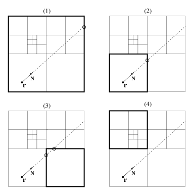
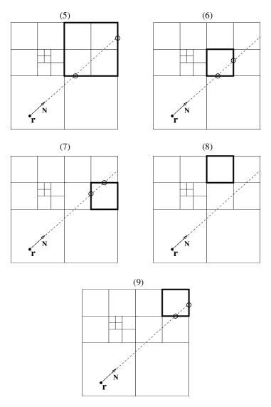
Figure 7: An illustration of how the optical depth between the outer boundary (the largest cell) and the current location ($\mathbf{r}$) of the photon moving in the direction $\mathbf{N}$ is calculated. The corresponding instructions for each step are summarized in § 2.7. The thick solid lines indicate the important cell in each step. The filled circle is the current location the photon, and the open circles are the intersections of the photon beam and the cell of current interest.

If the cell sizes and their locations are chosen properly, the accuracy of the optical depth value is within a few percent in normal runs of our models. This method is used because of the simplicity and the speed. On the other hand, if accuracy of the optical depth value is crucial, we can use neighboring cell values to improve the optical depth estimate. Computing the optical depth is the most time consuming part of the code.

3 Tests

3.1 Continuum Polarization Tests

Firstly, the continuum polarization arising from an optically thin envelope of a single star is examined. The light source is assumed to be a point source which is embedded in the density of the following form.

$$\rho(r,\theta)=\rho_{o}\,\frac{1}{r^{2}}\,a\,\left(1+b\cos^{2}\theta\right)\,$$ (7)

where $\rho_{o}$ is a constant, $a$ is an angular normalization constant and $b$ is the parameter which controls the angular dependency of $\rho$. When $b$ is $<0$, $=0$, and $>0$, the stellar envelope is oblate, spherical, and prolate respectively. The opacity of the atmosphere is set to be $\tau\approx 0.1$. In Fig. 8, the normalized polarization levels computed as a function of inclination angle are shown, and they are compared with the predictions from the model of Brown & McLean (1977). $b=-0.5$ is used in both models. The figure shows that the results from the two models are in excellent agreement.

Secondly, a binary system which consists of two identical point sources orbiting in a circular orbit is considered. Around each light source, a uniform spherical density is placed. Again, the envelopes are set to be optically thin so that the variation of polarization level can be compared with the binary polarization model of Brown et al. (1978). Fig. 9 shows that the results from the two models agree each other very well for three inclination angles ($i=0^{\circ},\,45^{\circ},\,90^{\circ}$).

Thirdly, we verified the computations against the 2-D Monte Carlo polarization model of Hillier (1991) and the 2-D radiative transfer codes of Hillier (1994) whose models allow for multiple scatterings (optically thick) and an extended source. Our results are in good agreement with both models i.e., $I$ and $Q$ are within a fractional error of 0.01.

Figure 8: Comparison of the polarization v.s. inclination angle of a oblate atmosphere around a single star according to the model of Brown & McLean (1977) (lines) and our model (circles). The model consist of a point source embedded in the density in the form of Eq. 7. The result from our model agrees with the analytic solution of Brown & McLean (1977) very well.

Figure 9: Comparison of Q & U polarization double sine curves predicted by the analytic model of Brown et al. (1978) and our models for three different inclination angles. Two identical point sources, which are orbiting around each other in a circular orbit, are each embedded in an optically thin spherical envelope. The points with makers are from our model, and the lines are from the model of Brown et al. (1978): Circles follow $i=0^{\circ}$ (face-on) curve, squares follow $i=45^{\circ}$, and diamonds follow $i=90^{\circ}$ (edge-on) curve. The agreement of the two models is excellent for all inclination angles. The small deviations of our model from that of Brown et al. (1978) around phase $=0.42$ and $0.58$ for $i=90^{\circ}$ is due to the atmospheric eclipse since the model of Brown et al. (1978) did not include the attenuation of the star light before scatterings.

3.2 Line Polarization Tests

A He i ($\lambda 5411$) line emitted from a single WN type star ($R=1.5R_{\sun}$, $L=2.0\times 10^{5}\,L_{\sun}$, $\dot{M}=0.6\times 10^{-5}\,M_{\sun}\,\mathrm{yr}^{-1}$) is computed with the 3-D Monte Carlo code and the 2-D radiative transfer codes of Hillier (1996). The angular dependency of the atmosphere is assumed to be the same as in Eq. 7 with $b=-0.5$. Fig. 10 shows the results from both models are in excellent agreement.

An example of a non-axisymmetric system is a rotating atmosphere of a single star. Although density distribution is usually symmetric around a rotation axis, the velocity field is not axisymmetric. To examine a basic behavior of polarization variations across an emission line, the following two simple models are computed. 1. an expanding atmosphere (beta velocity law with $\beta=0.5$, $V_{\infty}=500\,\mathrm{km}\,\mathrm{s}^{-1}$) and 2. an expanding & rotating atmosphere (beta-velocity law$+$solid-body rotation with $V_{\mathrm{rot}}=182\,\mathrm{km}\,\mathrm{s}^{-1}$ on the stellar surface). The results are shown in Fig. 11. Qualitatively, the behavior of these line variations are the same as those described by McLean (1979) (in their Figure 5), and those of a simple analytical model by Wood et al. (1993) (in their Figs. 4, 6 and 8).

Figure 10: A model of an optically thick He ii ($\lambda 5411$) line for a WN5 type star. Normalized flux (top), percentage polarization (middle) and polarization angle (bottom) were computed by our 3-D Monte Carlo model (solid), and compared with the 2-D radiative transfer model (dotted) of Hillier (1996). The angular distribution of electron gas is assumed to be the same as in Eq. 7 with $b=-0.5$. The agreement between the two models is excellent.

Figure 11: The effect of rotation on line polarization is demonstrated in this diagram. Solid line: an emission line produced by a radially expanding atmosphere. Dotted line: same emission line, but solid-body rotation is added to the expanding atmosphere. An inclination angle of $60^{\circ}$ was used for both models. The angular distribution of electrons was assumed to be the same as in Eq. 7 with $b=-0.5$.

4 Example Calculations for a Binary System: V444 Cyg

As an application to a real system, the phase dependent Stokes parameters $\left(I,\,Q,\,U\right)$ of the massive binary system V444~Cyg (WN5+O6 III-V) are computed with our model. The system is a short-period ($P=4.212$ days, Khaliullin et al. 1984) eclipsing binary, and it exhibits variability in polarization, line strength and X-ray flux as a function of orbital phase. The variability arises from occultation of the photosphere, from perturbations induced in the extended atmosphere of the W-R star by the O star and its wind, and from the wind-wind interaction region. Despite the complexities, many authors (e.g., Hamann & Schwarz 1992; St-Louis et al. 1993; Marchenko et al. 1994; Cherepashchuk et al. 1995; Moffat & Marchenko 1996; Marchenko et al. 1997; Stevens & Howarth 1999, and etc.) have used this object to determine fundamental parameters of the W-R star by taking advantage of its variable nature.

The model consists of three main components: 1. the W-R star atmosphere, 2. the O star’s spherical surface (with a limb-darkening law) and 3. the paraboloid-shaped bow shock region due to the colliding stellar winds (Fig. 12). More detailed discussion on the V444~Cyg polarization model can be found in Kurosawa & Hillier (2001). Fig. 13 shows the resulting continuum Stokes parameters $\left(I,\,Q,\,U\right)$ at $5630$Å as a function of orbital phase. The model reproduces the eclipsing $I$ light curve, the double sine curves of $Q$ & $U$ polarizations and the small oscillations seen in $Q$ & $U$ near the secondary eclipse (phase=0.5). Next, the phase dependent He i ($\lambda$5876) emission line, created mainly in the outer part of the W-R atmosphere in the binary, is computed. The results are shown in Fig. 14. The left plot in Fig. 14 shows the sequence of He i ($\lambda$5876) line profiles computed with unrealistically high emissivity in the bow shock region, to emphasize the effect of the bow shock. The underlying ordinary He i emission from the W-R star is barely visible in this plot. On the left in Fig. 14, the sequence of the same line is displayed, but with a more realistic amount of emission from the bow shock region. This figure qualitatively describes the variability seen in the observation of this line (see e.g., Marchenko et al. 1994).

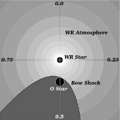
Figure 12: This figure illustrates the model configuration of V444~Cyg (WN5+O6 III-V) on the orbital plane. The W-R star is placed at the center of the cubic boundary, and it is surrounded by the spherical atmosphere. The O star is located below the W-R star in the diagram, and the tilted paraboloid shock with a given thickness is covering the O star. The strong stellar wind from the W-R star is interrupted by the shock front, and the density behind the shock is assumed to be insignificantly small for simplicity. The direction to an observer at phase $=0,\,0.25,\,0.5,\,0.75$ are indicated at the top, bottom, left and right edges since the orbital inclination is about $80^{\circ}$ (almost edge-on view).

Figure 13: The figure shows the model calculation of polarization light curves for V444 Cyg. The relative flux (top), $Q$ (middle) and $U$ (bottom) polarization at $\lambda=5630$Å, as a function of binary phase, are plotted. Circle: observation, Solid: our model with $\dot{M}=0.6\times 10^{-5}\,M_{\sun}yr^{-1}$. The optical light curve data and optical polarization data are from Kron & Gordon (1943) and St-Louis et al. (1993) respectively.

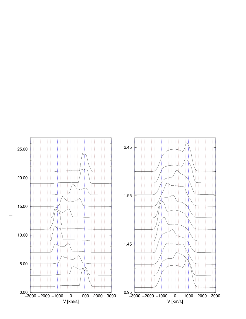
Figure 14: Left: Shows the phase dependent emission from the bow shock region (see Fig. 12) seen on the top of He i ($\lambda 5876$) line. The emissivity of the bow shock region is set to be unrealistically strong in order to demonstrate the effect of the bow shock emission. Right: Same as for the left figure, but the emissivity of the bow shock region is reduced by a factor of $\sim 10$. This figure qualitatively describes the variability seen in the observation of this line (see e.g., Marchenko et al. 1994). The profiles are plotted from phase $=0$ (bottom) to phase $=1$ (top) with $0.1$ phase steps.

5 Conclusions

We have presented a new 3-D Monte Carlo model which computes the variability in line and continuum polarization associated with the orbital motion of a binary system surrounded by a non-axisymmetric envelope. The basic model is constructed in a general manner so that it can handle an arbitrary distribution of gas density. A special method of grid spacing called the “cell-splitting” method is used to automatically assign more grid points to the higher density regions. For a fixed number of grid points, the tree method achieves a higher accuracy than the uniform cubic grid method. This kind of grid scheme is very useful in multi-dimensional calculations. It is not restricted to a binary system, but also applicable to many other astrophysical systems, e.g., accretion flows, molecular clouds and a 3-D hydrodynamical model.

The model was tested extensively. We demonstrated the accuracy of our model by comparing it with simple analytical models and existing well-tested 2-D numerical models. Firstly, the model was tested against the analytic models of continuum polarization by Brown & McLean (1977) and Brown et al. (1978), and they were in excellent agreement for both a point source and a binary model. Secondly, the polarization in the optically thick He ii ($\lambda 5411$) line calculated by our model and by the 2-D radiative transfer model of Hillier (1996) were compared. They also showed good agreement. Thirdly, the effect of rotation on the line polarization seen in an emission line was demonstrated. The basic behavior of polarization and polarization angle across an emission line, computed by our model, are confirmed to be the same as those in McLean (1979) and Wood et al. (1993).

We also demonstrated the application of our model to a real system: V444~Cyg. The model was able to produce a set of complicated $I$, $Q$ and $U$ light curves which fit the observational data very well. In addition, we qualitatively modeled the phase dependent excessive emission seen on the top of the optically thin He i ($\lambda 5976$) line. Since this excessive emission is originated from the bow shock heated region due to the colliding stellar winds, by modeling the sequence of this line properly, we would be able to probe little known properties (e.g., gas flow, geometrical configuration) of the bow shock in the system. If one wishes to model a line variability associated with the bow-shock region correctly, one needs to have realistic opacity information in the region. A more formal approach to this kind of problem is to develop a full 3-D non-LTE radiative transfer model. Because of the high dimensionality, computational time would increase much more than in the case of a 1-D problem. Developing a 3-D Monte Carlo non-LTE radiative transfer model would be simpler than developing the 3-D short-characteristic ray method e.g., by Folini & Walder (1999), and the tree data structure is relevant to this problem.

In a following paper (Kurosawa & Hillier 2001), we will apply our model, in conjunction with the multi-line non-LTE radiative transfer model of Hillier & Miller (1998), to estimate the mass-loss rate of V444~Cyg. This will be done by fitting the observed He i ($\lambda 5876$) and He ii ($\lambda 5412$) line profiles, and the continuum light curves of three Stokes parameters $\left(I,\,Q,\,U\right)$ in $V$ band simultaneously.

References

- Bernes (1979) Bernes, C. 1979, A&A, 73, 67
- Brown et al. (1989) Brown, J. C., Carlaw, V. A., & Cassinelli, J. P. 1989, ApJ, 344, 341
- Brown & McLean (1977) Brown, J. C. & McLean, I. S. 1977, A&A, 57, 141
- Brown et al. (1978) Brown, J. C., McLean, I. S., & Emslie, A. G. 1978, A&A, 68, 415
- Chandrasekhar (1960) Chandrasekhar, S. 1960, Radiative transfer (New York: Dover, 1960)
- Cherepashchuk et al. (1995) Cherepashchuk, A. M., Koenigsberger, G., Marchenko, S. V., & Moffat, A. F. J. 1995, A&A, 293, 142
- Folini & Walder (1999) Folini, D. & Walder, E. 1999, in IAU Symp., Vol. 193, Wolf-Rayet Phenomena in Massive Stars and Starburst Galaxies, ed. K. A. van der Hucht, G. Koenigsberger, & P. R. J. Eenens, 352
- Gayley et al. (1997) Gayley, K. G., Owocki, S. P., & Cranmer, S. R. 1997, ApJ, 475, 786
- Hamann & Schwarz (1992) Hamann, W. R. & Schwarz, E. 1992, A&A, 261, 523
- Harries (2000) Harries, T. J. 2000, MNRAS, 315, 722
- Hillier (1991) Hillier, D. J. 1991, A&A, 247, 455
- Hillier (1994) —. 1994, A&A, 289, 492
- Hillier (1996) —. 1996, A&A, 308, 521
- Hillier & Miller (1998) Hillier, D. J. & Miller, D. L. 1998, ApJ, 496, 407
- Juvela (1997) Juvela, M. 1997, A&A, 322, 943
- Khaliullin et al. (1984) Khaliullin, K. F., Khaliullina, A. I., & Cherepashchuk, A. M. 1984, Soviet Astron. Lett., 10, 250
- Koenigsberger & Auer (1985) Koenigsberger, G. & Auer, L. H. 1985, ApJ, 297, 255
- Kron & Gordon (1943) Kron, G. E. & Gordon, K. C. 1943, ApJ, 97, 311
- Kurosawa & Hillier (2001) Kurosawa, R. & Hillier, D. J. 2001, ApJ, submitted
- Li & McCray (1996) Li, H. & McCray, R. 1996, ApJ, 456, 370
- Lucy (1999) Lucy, L. B. 1999, A&A, 345, 211
- Luo et al. (1990) Luo, D., McCray, R., & Mac Low, M. 1990, ApJ, 362, 267
- Marchenko et al. (1997) Marchenko, S. V., Moffat, A. F. J., Eenens, P. R. J., Cardona, O., Echevarria, J., & Hervieux, Y. 1997, ApJ, 422, 810
- Marchenko et al. (1994) Marchenko, S. V., Moffat, A. F. J., & Koenigsberger, G. 1994, ApJ, 422, 810
- McLean (1979) McLean, I. S. 1979, MNRAS, 186, 265
- Modali et al. (1972) Modali, S. B., Brandt, J. C., & Kastner, S. O. 1972, ApJ, 175, 265
- Moffat & Marchenko (1996) Moffat, A. F. J. & Marchenko, S. V. 1996, A&A, 305, L29
- Pagani (1998) Pagani, L. 1998, A&A, 333, 269
- Pittard (1998) Pittard, J. M. 1998, MNRAS, 300, 479
- Pittard & Stevens (1999) Pittard, J. M. & Stevens, I. R. 1999, in IAU Symp., Vol. 193, Wolf-Rayet Phenomena in Massive Stars and Starburst Galaxies, ed. K. A. van der Hucht, G. Koenigsberger, & P. R. J. Eenens (San Francisco, Calif: Astronomical Society of the Pacific), 386
- Sandford (1973) Sandford, M. T. 1973, ApJ, 183, 555
- Shore & Brown (1988) Shore, S. N. & Brown, D. N. 1988, ApJ, 334, 1021
- St-Louis et al. (1993) St-Louis, N., Moffat, A. F. J., Lapointe, L., Efimov, Y. S., Shakhovskoj, N. M., Fox, G. K., & Piirola, V. 1993, ApJ, 410, 342
- Stevens et al. (1992) Stevens, I. R., Blondin, J. M., & Pollock, A. M. T. 1992, ApJ, 386, 265
- Stevens & Howarth (1999) Stevens, I. R. & Howarth, I. D. 1999, MNRAS, 302, 549
- Stevens & Pollock (1994) Stevens, I. R. & Pollock, A. M. T. 1994, MNRAS, 269, 226
- Warren-Smith (1983) Warren-Smith, R. F. 1983, MNRAS, 205, 337
- Witt & Gordon (1996) Witt, A. N. & Gordon, K. D. 1996, ApJ, 463, 681
- Wolf et al. (1999) Wolf, S., Henning, T., & Stecklum, B. 1999, A&A, 349, 839
- Wood et al. (1993) Wood, K., Brown, J. C., & Fox, G. K. 1993, A&A, 271, 492