Numerical evolutions of nonlinear $r$-modes in neutron stars

Abstract

Nonlinear evolution of the gravitational radiation (GR) driven instability in the $r$-modes of neutron stars is studied by full numerical 3D hydrodynamical simulations. The growth of the $r$-mode instability is found to be limited by the formation of shocks and breaking waves when the dimensionless amplitude of the mode grows to about three in value. This maximum mode amplitude is shown by numerical tests to be rather insensitive to the strength of the GR driving force. Upper limits on the strengths of possible nonlinear mode–mode coupling are inferred. Previously unpublished details of the numerical techniques used are presented, and the results of numerous calibration runs are discussed.

I Introduction

In recent years the gravitational radiation (GR) driven instability in the $r$-modes of rotating neutron stars has received considerable interest, both as a source of gravitational waves for detectors such as the Laser Interferometer Gravitational Wave Observatory (LIGO), and as an astrophysical process capable of limiting the rotation rates of neutron stars. In any rotating star, the $r$-modes are driven towards instability by GR Andersson98 ; Friedman98 : as the star emits gravity waves (primarily through a gravitomagnetic effect), the GR reaction acts back on the fluid by lowering the (already negative) angular momentum of the mode. This in turn causes the amplitude of the mode to grow. In most stars internal dissipation suppresses the $r$-mode instability, but this may not be the case for hot, rapidly rotating neutron stars Lindblom98 ; Lindblom01b . For neutron stars with millisecond rotation periods, the timescale for the growth of the instability is about 40 s. In the absence of any limiting process, GR would force the dimensionless amplitude of the most unstable ($m=2$) $r$-mode to grow to a value of order unity within about ten minutes of the birth of such a star. (At unit amplitude, the characteristic $r$-mode velocities are comparable to the rotational velocity of the star.)

The strength of the GR emitted and the timescale on which the neutron star loses angular momentum and spins down depend critically on the maximum amplitude to which the $r$-mode grows. Initial estimates assumed that the amplitude would grow to a value of order unity before an undescribed nonlinear process saturated the mode. After saturation, it was assumed that the spindown would proceed as a quasi-stationary process, reducing the angular velocity to one tenth of its initial value within about one year. In this scenario, gravitational waves from spindown events might be detectable with LIGO II Owen98 .

However, at present no one knows with certainty how large the amplitude of the $r$-modes will grow. It may well be that the nonlinear hydrodynamics of the star might limit the growth of $r$-modes to very small values. This could happen, for instance, if the $r$-modes were to leak energy by nonlinear coupling into other modes faster than GR reaction could restore it. In this case the $r$-mode instability would not play any interesting role in real astrophysical systems.

In a previous paper Lindblom01 , we presented the preliminary results of fully nonlinear, three-dimensional numerical simulations aimed at investigating the growth of $r$-modes. In our simulations, we modeled a young neutron star as a rapidly rotating, isentropic, Newtonian polytrope; we added a small-amplitude seed $r$-mode and we solved the hydrodynamic equations driven by an effective GR reaction force. We found that $r$-mode saturation intervenes at amplitudes far larger than expected ($\sim 3$), supporting the astrophysical relevance of $r$-modes and the possibility of detecting $r$-mode gravity waves. The details of the GR signature emitted by the $r$-mode instability that we observe in our simulations are rather different than previously envisioned, and these details suggest that this radiation may be more easily detected than previously thought: the radiation is more monochromatic and is emitted in a shorter, more powerful burst (see Ref. Lindblom01 and the final Section of this paper).

Our results are compatible with the conclusions of Stergioulas and Font Stergioulas01 , who performed relativistic simulations of $r$-modes on a fixed neutron-star geometry, and found no saturation even at large amplitudes. A second point of comparison can be made with the work of Schenk and colleagues Schenk01 . They have attacked the problem analytically, developing a perturbative formalism to study the nonlinear interactions of the modes of rotating stars, and proving that the couplings of $r$-modes to many other rotational modes are small (they are forbidden by selection rules, or they vanish to zeroth order in the angular velocity of the star).

The present work is meant as a complement to Ref. Lindblom01 : throughout these pages, we describe our simulations in greater detail; we discuss their relevance and their limitations in the light of Refs. Stergioulas01 ; Schenk01 ; and we present the results of several additional simulations aimed at enlightening particular aspects of the problem. In Sec. II we write down the basic hydrodynamic equations, and we define a number of mathematical quantities that will be used to monitor the nonlinear evolution of the $r$-modes. In Sec. III we implement the effective current-quadrupole gravitational radiation-reaction force. In Sec. IV we integrate the fluid equations with $r$-mode initial data in slowly rotating stars, and we compare the results with the small-amplitude, slow-rotation analytical expressions: we demonstrate that the integration reproduces faithfully the analytical predictions to the expected degree of accuracy. In Secs. V–VIII we study the nonlinear evolution of $r$-mode initial data in rapidly rotating stars, concentrating on the nonlinear saturation of the $r$-modes, and analyzing in detail the evolution of several hydrodynamical quantities. Finally, we summarize our conclusions in Sec. IX.

II Basic Hydrodynamics

We study the solutions to the Newtonian fluid equations,

$$\partial_{t}\rho+\vec{\nabla}\cdot\bigl{(}\rho\vec{v}\bigr{)}=0,$$ (1)

$$\rho\bigl{(}\partial_{t}\vec{v}+\vec{v}\cdot\vec{\nabla}\vec{v}\bigr{)}=-\vec{\nabla}p-\rho\vec{\nabla}\Phi+\rho\vec{F}^{\mathrm{GR}},$$ (2)

$$\partial_{t}\tau+\vec{\nabla}\cdot\bigl{(}\tau\vec{v}\bigr{)}=0,$$ (3)

where $\vec{v}$ is the fluid velocity, $\rho$ and $p$ are the density and pressure, $\Phi$ is the Newtonian gravitational potential, and $\vec{F}^{\mathrm{GR}}$ is the gravitational radiation reaction force. Equation (3) is a recasting of the energy equation for adiabatic flows, where $\tau$ is the entropy tracer Tohline01 ; for polytropic equations of state, $\tau$ is related to the internal energy (per unit mass) $\epsilon$ by the relation $\tau=(\epsilon\rho)^{1/\gamma}$, where $\gamma$ is the adiabatic exponent. The Newtonian gravitational potential is determined by Poisson’s equation,

$$\nabla^{2}\Phi=4\pi G\rho,$$ (4)

while the gravitational radiation reaction force will be discussed in Sec. III.

We solve Eqs. (1)–(4) numerically in a rotating reference frame, using the computational algorithm developed at LSU to study a variety of astrophysical hydrodynamic problems Tohline97 . The code performs an explicit time integration of the equations using a finite-difference technique that is accurate to second order both in space and time, and uses techniques very similar to those of the familiar ZEUS code Stone92 . For most of our simulations, we adopt a cylindrical grid with 64 cells in the radial direction, and 128 cells in the axial and azimuthal directions.

In the limit of slow rotation, we define the $r$-modes of rotating Newtonian stars (using the normalization of Lindblom, Owen and Morsink Lindblom98 ) as the solutions of the perturbed fluid equations having the Eulerian velocity perturbation

$$\delta\vec{v}=\alpha_{0}R\Omega_{0}\Bigl{(}\frac{r}{R}\Bigr{)}^{l}\vec{Y}^{B}_{ll}e^{i\omega_{0}t},$$ (5)

where $R$ and $\Omega_{0}$ are the radius and angular velocity of the unperturbed star, $\alpha_{0}$ is the dimensionless $r$-mode amplitude, and $\vec{Y}^{B}_{ll}$ is a vector spherical harmonic of the magnetic type, defined by

$$\vec{Y}^{B}_{lm}=[l(l+1)]^{-1/2}r\vec{\nabla}\times(r\vec{\nabla}Y_{lm}).$$ (6)

The $r$-mode frequency is given by Papaloizou78

$$\omega_{0}=-\frac{(l-1)(l+2)}{l+1}\Omega_{0}.$$ (7)

To monitor the nonlinear evolution of the $r$-modes, it is helpful to introduce nonlinear generalizations of the amplitude and frequency of the mode. These quantities are defined most conveniently in terms of the current multipole moments of the fluid,

$$J_{lm}=\int\rho r^{l}\vec{v}\cdot\vec{Y}^{B*}_{lm}d^{3}x.$$ (8)

In slowly rotating stars, the $J_{22}$ moment is proportional to the amplitude of the $m=2$ $r$-mode, the most unstable mode, and the one that we will study. To track the evolution of this mode even in the nonlinear regime, we define the normalized, dimensionless amplitude

$$\alpha=\frac{2|J_{22}|}{\tilde{J}MR^{3}\Omega_{0}},$$ (9)

where $M$ is the total mass of the star and $\tilde{J}$ is defined by

$$\tilde{J}MR^{4}=\frac{1}{4\pi}\int\rho r^{4}d^{3}x\simeq\int\rho r^{6}dr.$$ (10)

The quantity $\tilde{J}$ is evaluated once and for all at the beginning of each of our evolutions. For slowly rotating stars, the definition (9) of the mode amplitude reduces to the one given by Eq. (5).

In slowly rotating stars, and in all situations where the leading contribution to $J_{22}$ comes from the $m=2$ $r$-mode, the time derivative $dJ_{22}/dt$ is proportional to the frequency of the mode: $d{J}_{22}/dt=i\omega J_{22}$. Thus we are led to define the nonlinear generalization of the $r$-mode frequency as

$$\omega=-\frac{1}{|J_{22}|}\left|\frac{d{J}_{22}}{dt}\right|.$$ (11)

As shown by Rezzolla, et al. Rezzolla99 , we can re-express $dJ_{22}/dt$ as an integral over the standard fluid variables,

$$J^{(1)}_{22}\equiv\frac{d{J}_{22}}{dt}=\int\rho\Bigl{[}\vec{v}\cdot\bigl{(}\vec{\nabla}\vec{Y}^{B*}_{22}\bigr{)}\cdot\vec{v}-\vec{\nabla}\Phi\cdot\vec{Y}^{B*}_{22}\Bigr{]}d^{3}x.$$ (12)

The definitions, Eqs. (9) and (11), of mode amplitude and mode frequency are very stable numerically, because they are expressed in terms of integrals over the fluid variables. In the Appendix, we give explicit expressions for $J_{22}$ and $J^{(1)}_{22}$ in the cylindrical coordinate system used in our numerical analysis.

While we monitor the nonlinear evolution of the $r$-mode, we are also interested in tracking the star’s average angular velocity as well as its degree of differential rotation. With this in mind, we define the average angular velocity

$$\bar{\Omega}\equiv J/I,$$ (13)

where the angular momentum and the moment of inertia are given respectively by

$$J=\int\rho\varpi^{2}\Omega(\varpi,z,\varphi)d^{3}x,$$ (14)

$$I=\int\rho\varpi^{2}d^{3}x.$$ (15)

Here $\varpi$ is the cylindrical radial coordinate, and the local angular velocity $\Omega(\varpi,z,\varphi)\equiv v_{\hat{\varphi}}/\varpi$, where $v_{\hat{\varphi}}$ is the proper azimuthal component of the fluid velocity. We also define the average differential rotation $\Delta\Omega$ as the weighted variance of $\Omega$,

$$\bigl{(}\Delta\Omega\bigr{)}^{2} = I^{-1}\int\rho\varpi^{2}\bigl{(}\Omega-\bar{\Omega}\bigr{)}^{2}d^{3}x$$ (16)

$$= I^{-1}\int\rho\varpi^{2}\Omega^{2}d^{3}x-\bar{\Omega}^{2}.$$

III Radiation-Reaction Force

The gravitational radiation-reaction force due to a time-varying current quadrupole is given by the expression

$$\!\!\!\!\!\!\!\!\!F^{\mathrm{GR}}_{a} = \kappa\frac{16}{45}\frac{G}{c^{7}}\biggl{(}2v_{j}\epsilon_{jal}x_{m}S^{(5)}_{lm}+v_{j}\epsilon_{jkl}x_{k}S^{(5)}_{la}$$ (17)

$$\qquad\quad-v_{j}\epsilon_{akl}x_{k}S^{(5)}_{lj}-\epsilon_{akl}x_{k}x_{m}S^{(6)}_{lm}\biggr{)},$$

see Blanchet Blanchet97 , and Eq. (20) of Rezzolla et al. Rezzolla99 . Here $S^{(n)}_{jk}$ represents the $n$’th time derivative of the current quadrupole tensor,

$$S_{jk}=\int\rho(\vec{x}\times\vec{v})_{(j}x_{k)}d^{3}x;$$ (18)

$\epsilon_{jkl}$ is the totally antisymmetric tensor, and the vector $x_{k}$ represents the Cartesian coordinates of the point at which the force is evaluated. The parameter $\kappa$ that appears in Eq. (17) has the value $\kappa=1$ in general relativity. For reasons discussed below, we find it useful to consider other values of $\kappa$ in our numerical simulations.

We find that a straightforward application of Eq. (17) in numerical evolutions is nearly impossible. There are two problems: first, it is very hard to evaluate reliably time derivatives of such a high order; second, various sources of numerical noise (even small errors in the initial equilibrium configuration of the fluid, and the numerical drift of the center of mass) can generate contributions to the current quadrupole tensor that overwhelm those of the pure $r$-mode motion. So we need to introduce special numerical techniques and simplifications to overcome these problems.

In order to reduce the influence of extraneous noise sources on the evolution, it is helpful to re-express the current quadrupole tensor in terms of the current multipole moments defined in Eq. (8). There is a one-to-one correspondence between the $J_{2m}$ current multipoles and $S_{ij}$:

$$S_{yy}-S_{xx}+2iS_{xy} = \sqrt{\frac{16\pi}{5}}J_{22},$$ (19)

$$S_{xz}-iS_{yz} = \sqrt{\frac{4\pi}{5}}J_{21},$$ (20)

$$S_{xx}+S_{yy}=-S_{zz} = \sqrt{\frac{8\pi}{15}}J_{20}.$$ (21)

In a slowly rotating star, the $m=2$ $r$-mode excites $J_{22}$, but not $J_{21}$ and $J_{20}$. In contrast, the principal sources of numerical noise contribute primarily to $J_{20}$. Thus, we evaluate only the $J_{22}$ contribution to $\vec{F}^{\mathrm{GR}}$: we use Eq. (17) to evaluate $\vec{F}^{\mathrm{GR}}$, taking the $S_{ij}$ determined from Eqs. (19)–(21), but setting $J_{21}=J_{20}=0$. We find that this scheme reduces considerably the numerical noise in the radiation reaction force, and reproduces faithfully the analytical description of $r$-modes in slowly rotating stars (see Sec. IV).

The second major problem is evaluating the numerical time derivatives of $S_{jk}$, or equivalently the time derivatives of $J_{22}$. Whenever the radiation-reaction timescale is much longer than the $r$-mode period $2\pi/\omega$, the dominant contribution to the derivatives $S^{(n)}_{jk}$ comes from terms proportional to powers of the $r$-mode frequency:

$$S^{(n)}_{jk}\approx(i\omega)^{n}S_{jk},\quad J^{(n)}_{22}\approx(i\omega)^{n}J_{22}.$$ (22)

Even when the $r$-mode amplitude becomes large, the expression (22) will be accurate as long as the timescale for the evolution of $\alpha$ and $\omega$ is longer than $2\pi/\omega$. Now, $J_{22}$ and $J^{(1)}_{22}$ are easily evaluated using the integral expressions in Eqs. (8) and (12); thus, the time derivatives needed in Eq. (17) are given simply by $J^{(5)}_{22}=\omega^{4}J^{(1)}_{22}$ and $J^{(6)}_{22}=-\omega^{6}J_{22}$, where we determine $\omega$ numerically using Eq. (11). In the Appendix, we present explicit expressions for the components of the effective radiation-reaction force in cylindrical coordinates.

IV Calibration runs

In order to test the accuracy of our hydrodynamic evolution code and of our approximations for the gravitational radiation-reaction force, we investigate the evolution of a small-amplitude $r$-mode in a slowly rotating star.

We provide initial data for this study by solving the time-independent fluid equations for a slowly, rigidly rotating stellar model. We model the neutron star as an $n=1$ polytrope, generated by the self consistent field technique developed by Hachisu Hachisu86 . Table 1 shows the physical parameters for this model, labeled Slow; in particular, the ratio of rotational kinetic energy to gravitational binding energy is $T_{\mathrm{rot}}/|W|=0.00398$, and the angular velocity is 26% of the maximum possible value (estimated as $\Omega_{\mathrm{max}}=\frac{2}{3}\sqrt{\pi G\bar{\rho}}$).

Table 1: Physical parameters for the equilibrium models.

Parameter	Symbol	Slow	Fast
		C1, C2	C3–C8
polytropic index	$n$	1	1
total mass	$M$	$1.4\,M_{\odot}$	$1.4\,M_{\odot}$
equatorial radius	$R_{\mathrm{eq}}$	12.7 km	18.4 km
polar R/equatorial R	$R_{\mathrm{pol}}/R_{\mathrm{eq}}$	0.98	0.59
nonrotating R	$R_{0}$	12.5 km	12.5 km
angular velocity	$\Omega_{0}$	1.45 krad/s	5.34 krad/s
rotation period	$P_{0}$	4.32 ms	1.18 ms
energy ratio	$T_{\mathrm{rot}}/|W|$	$3.98\times 10^{-3}$	0.10072
simulation RR timescale	$\tau^{(s)}_{\mathrm{RR}}$	$0.459\,P_{0}$	$9.4374\,P_{0}$
physical RR timescale	$\tau^{(p)}_{\mathrm{RR}}$	$2.8\times 10^{7}P_{0}$	$4.2\times 10^{4}P_{0}$

We then adjust the velocity field of this equilibrium model by adding the velocity perturbation of an $m=2$ $r$-mode of amplitude $\alpha_{0}$:

$$\vec{v}=\varpi\Omega_{0}\vec{e}_{\hat{\varphi}}+\alpha_{0}R\Omega_{0}\left(\frac{r}{R}\right)^{2}{\mathrm{Re}}(\vec{Y}^{B}_{22}).$$ (23)

In the Appendix, we write out explicitly the components of this initial velocity field in our cylindrical coordinate system. Because Eq. (23) is the exact representation of a pure $m=2$ $r$-mode only in the small-amplitude, small-rotation limit, we expect that the frequency and the amplitude measured in our numerical experiment using Eqs. (9)–(11) will be different from their theoretical values $\alpha_{0}$ and $-\frac{4}{3}\Omega_{0}$ by terms of order $O(\alpha^{2})$, and $O(\Omega^{2}/\Omega_{\mathrm{max}}^{2})$.

We perform two numerical integrations of the equations of motion, for this slowly rotating initial configuration. In the first run (C1), we let the star evolve under purely Newtonian hydrodynamics, setting the strength $\kappa$ of the radiation reaction (17) to zero. In the second run (C2), we force the mode by setting $\kappa\simeq 6\times 10^{7}$. With this unphysically large value the amplitude of the $r$-mode grows appreciably within a time that we can conveniently follow numerically. (The Courant limit for the evolution timestep is set by the speed of sound in the fluid, and by the size of the grid cells; for $\Omega_{0}=0.26\Omega_{\mathrm{max}}$, one complete rotation of the star takes about 70000 timesteps).

Figure 1: Evolution of the $r$-mode amplitude in a slowly rotating star. The solid curves plot the results of numerical evolutions (with and without gravitational radiation reaction) while the dashed curves plot the analytical predictions. For the curves marked “free,” $\kappa=0$; for the curves marked “forced,” $\kappa\simeq 6\times 10^{7}$.

Figure 1 illustrates the evolution of the mode amplitude $\alpha$ in runs C1 and C2, as a function of $t/P_{0}$, where $P_{0}=2\pi/\Omega_{0}$ is the initial rotation period of the star. The solid curves trace the numerical evolution of $\alpha$ [as defined in Eq. (9)], whereas the dashed curves trace the theoretical predictions for this evolution, obtained in the small-amplitude, slow-rotation limit Lindblom98 .

When $\kappa=0$, the theoretical prediction for the evolution of the amplitude is just $\alpha=\alpha_{0}$, and we can verify that the numerical evolution tracks the analytical curve within the expected deviations of order $\alpha^{2}$. When $\kappa\neq 0$, the analytical prediction for the evolution of the amplitude is

$$\alpha=\alpha_{0}e^{t/\tau_{GR}},$$ (24)

where the radiation-reaction timescale is given by Lindblom98

$$\frac{1}{\tau_{\mathrm{GR}}}=2\pi\left(\frac{256}{405}\right)^{2}\kappa\frac{G}{c^{7}}\tilde{J}MR^{4}\Omega_{0}^{6}.$$ (25)

For this model, $\tau_{\mathrm{GR}}=0.46P_{0}$. As we can see in Fig. 1, the numerical evolution tracks the small-amplitude, slow-rotation analytical result within the expected accuracy, even if the radiation-reaction force is so unphysically strong.

Although this slow rotation numerical evolution was only carried out over a small fraction (0.2) of a rotation period (and therefore over a small fraction of the $r$-mode oscillation period), the evolution extended for about 7.3 dynamical times and 4.6 sound-crossing times.

Figure 2: Real and imaginary parts of the current multipole moment $J_{22}$ (in arbitrary units), for a slowly rotating star evolved without gravitational radiation reaction (run C1). The solid curves trace the numerical evolutions, the dashed curves trace the analytical predictions.

In Figs. 2 and 3, we display two additional diagnostics for the undriven ($\kappa=0$) slow-rotation evolution (C1). In Fig. 2 we plot the real and imaginary parts of the current multipole moment $J_{22}$: the solid curves trace the numerical evolution, whereas the dashed curves trace the analytical expression

$$J_{22}=\frac{1}{2}\alpha MR^{3}\tilde{J}\Omega_{0}e^{i\omega t}.$$ (26)

Again the deviations are within the expected accuracy of the analytical results. The deviations appear to be caused by the excitation of modes other than the pure $m=2$ $r$-mode; the spurious excitations appear because the initial data [Eq. (23)] are only accurate to first order in $\alpha$. Figure 3 depicts the evolution of the frequency $\omega$ [as defined in Eq. (11)]. The deviations from the analytical result, $\omega_{0}=-\frac{4}{3}\Omega_{0}$, are within the expected accuracy. The magnified scale used to display $\omega$ in Fig. 3 makes the presence of the small-amplitude, short-period extraneous modes quite apparent.

Figure 3: Frequency of the $m=2$ $r$-mode, for a slowly rotating star evolved without gravitational radiation reaction (run C1). The solid curve is determined numerically from Eq. (11). For comparison, the dashed line shows the analytical value $\omega_{0}=-\frac{4}{3}\Omega_{0}$.

V Evaluating the saturation amplitude

In our production runs, we investigate the nonlinear behavior of the $r$-mode in a rapidly rotating stellar model, under a variety of physical conditions (different initial amplitudes, and different values for the radiation-reaction coefficient $\kappa$).

Again, we provide initial data by solving the time-independent fluid equations for an $n=1$ polytrope. The physical parameters for this model, labeled Fast, are reported in Table 1; in particular, the ratio of rotational kinetic energy to gravitational binding energy is $T_{\mathrm{rot}}/|W|=0.10072$, and the angular velocity is 95% of its maximum value.

We perform a numerical integration of the equations of motion starting from the rapidly rotating initial configuration, Fast, using Eq. (23) to add a slow-rotation, small-amplitude $r$-mode field, with $\alpha_{0}=0.1$. Because the radiation-reaction force is so much stronger for this model (it is proportional to $\omega^{6}\propto\Omega^{6}$), we find that we can set $\kappa=4487$, which yields an $r$-mode growth time $\tau^{(s)}_{\mathrm{RR}}=9.43P_{0}$. This choice of $\kappa$ is still much larger than its physical value (unity), but it should yield a reasonable picture of the nonlinear evolution of the $r$-mode, if the timescales for all the relevant hydrodynamical processes (including nonlinear couplings to other modes) are comparable to $P_{0}$, or shorter. Indeed, if the average sound-crossing time $\tau_{S}$ is representative of the relevant hydrodynamical timescales, then our condition is satisfied: a rough estimate gives $\tau_{S}=R_{0}/\bar{c}_{S}\simeq 0.16P_{0}\simeq\tau^{(s)}_{\mathrm{RR}}/60$, where we have approximated $\bar{c}_{S}$ as the average speed of sound in the equivalent spherical polytrope.

Figure 4: Numerical evolution of $\mathrm{Re}\,J_{22}$ (arbitrary units) for a rapidly rotating star driven by gravitational radiation reaction (production run C3). The sinusoidal approximation, used to compute $\omega$ and $J_{22}^{(n)}$, is evidently appropriate for this run.

Figure 5: Numerical evolution of the $r$-mode amplitude $\alpha$ in production run C3.

V.1 Evolution of the $r$-mode amplitude

We follow the evolution through $t=33P_{0}$. Because the rotation of the star is progressively reduced by radiation reaction, and because the star develops differential rotation, at the end of the evolution the star has performed, on the average, only about 31 rotations [we obtain this number from $\int\bar{\Omega}dt/(2\pi)$]. In Fig. 4 we plot the numerically determined evolution of ${\rm Re}\,J_{22}$: the curve is a very smooth sinusoid, whose frequency is essentially constant, and whose envelope is determined by the (relatively slow) evolution of the $r$-mode amplitude. So the approximations used to compute $\omega$ and $J_{22}^{(n)}$ (discussed in Sec. III) are in fact quite good in this situation.

In Fig. 5 we plot the numerical evolution of the $r$-mode amplitude $\alpha$. At the beginning of the evolution, the computed diagnostic $\alpha$ agrees with the theoretical value $\alpha_{0}$ to $\sim$ 10%, within the expected accuracy. The growth is exponential (as predicted by perturbation theory) until $\alpha\approx 1.8$. Then some nonlinear process begins to limit the growth, until the amplitude peaks at $\alpha=3.35$ and then falls rapidly within a few rotation periods. After this the $r$-mode is effectively not excited.

V.2 A mechanism for $r$-mode saturation

What nonlinear process is responsible for the behavior of the $r$-mode amplitude? What causes the mode to saturate and disappear from the star? To answer these questions, we study the evolution of the total mass, total angular momentum, and total kinetic energy of the star, which are plotted in Fig. 6.

Figure 6: Evolution of total mass, total angular momentum, and total kinetic energy in production run C3. The quantities are plotted as fractions of their initial value.

Because the mass is constant, the damping of the $r$-mode cannot be caused by ejection of matter from the simulation grid. On the other hand, we expect that the star should lose energy and angular momentum as it radiates gravitational radiation in accord with the prediction of general relativity Rezzolla99 ; Thorne80 :

$$\left(\frac{dE}{dt}\right)_{\!J_{22}}=\frac{|\omega|}{2}\left(\frac{dJ}{dt}\right)_{\!J_{22}}=-\frac{128\pi}{225}\frac{G}{c^{7}}\kappa\omega^{6}|J_{22}|^{2}.$$ (27)

The evolution of the angular momentum mirrors this equation quite closely (within a few percent); for energy, however, Eq. (27) is only accurate until shortly after the catastrophic fall of the $r$-mode amplitude (at $t\simeq 28P_{0}$; see Fig. 7). Before that time, the star loses about 40% of its initial angular momentum and 36% of its initial kinetic energy. After that time, the amplitude and (therefore) the radiation-reaction force are much reduced, so $J$ becomes essentially constant; however, the kinetic energy continues to decrease, losing an additional 12% of its initial value during the next three rotation periods.

If the $r$-mode were damped by a hydrodynamical process that conserved energy, such as the transfer of energy to other modes, then Eq. (27) should portray accurately the evolution of the kinetic energy. But this is not what we see: instead, some purely hydrodynamic process continues to decrease the energy (by a sizable amount!) after the gravitational-radiation losses become negligible.

We believe that we have identified this process. To first order in the amplitude, the $r$-mode is only a velocity mode; to second order, however, there is also an associated density perturbation, proportional to $Y_{32}$, which appears as a wave with four crests (two in each hemisphere) on the surface of the star. (We will present a quantitative analysis later in this section.) As the amplitude reaches its maximum, these crests become large, breaking waves: the edges of the waves develop strong shocks that dump kinetic energy into thermal energy. In doing so they damp the $r$-mode. Figure 8 illustrates the surface waves at $t=28P_{0}$ and $t=29P_{0}$ along selected meridional slices.

Figure 7: Theoretical and numerical evolution of the total energy for production run C3. The total energy is plotted in units of the initial rotational energy (because the system is bound, $E_{\mathrm{tot}}$ must be negative).

Our code is written in such a way that the evolution of the shocks is always kinematically correct. In particular, the continuity equation ensures that mass is properly conserved, and that the proper density jump occurs across the shocks; and the Euler equation ensures that momentum is properly conserved, and that the proper pre- and post-shock velocities arise. However, our code does not allow the energy dissipated in the shock to increase the entropy of the fluid, which remains always barotropic and isentropic. Consequently, the presence of shocks shows up as a decrease in the total energy of the star. Indeed, in this production run (C3) gravitational radiation reduces the total energy by 9% of its initial magnitude through $t=28P_{0}$, and dissipation in shocks subtracts a further 3% in the last three rotations. (For comparison, 12% of the initial kinetic energy is lost in the last three rotations compared to 36% before that time.)

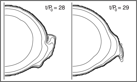
Figure 8: Isodensity surfaces showing breaking waves near the end of production run C3.

Ignoring the thermal effects of shocks is useful to reduce the computational burden and the complexity of the hydrodynamic code, and it is in fact a fairly reasonable approximation for neutron star matter, where the pressure comes mostly from the Fermi pressure of the degenerate neutrons, so the equation of state can be effectively modeled as temperature-independent.

V.3 Radial structure of the $r$-mode amplitude

We define the radial amplitude density $\alpha(r)$ (where $r$ is the spherical radius) by expressing the integral Eq. (8) for $J_{22}$ in spherical coordinates, and omitting the radial integration:

$$\alpha(r)e^{i\phi(r)}=\frac{2}{\tilde{J}MR^{2}\Omega_{0}}\int\rho r^{2}\vec{v}\cdot\vec{Y}^{B*}_{22}r^{2}\sin\theta d\theta\,d\varphi.$$ (28)

We removed the absolute value around the integral for $J_{22}$ so that we can keep track of the local mode phase $\phi(r)$. With this definition, $\alpha\exp[i\phi]=\int\alpha(r)\exp[i\phi(r)]dr/R$, where $\phi$ is the global phase of the $r$-mode.

The amplitude $\alpha(r)$ is plotted in Fig. 9 for the production run C3 at the time $t=22.5P_{0}$. Throughout the entire evolution, the mode is concentrated mostly between the spherical radii $r=0.5R$ and $0.9R$, and the shape of $\alpha(r)$ is fitted reasonably well by taking $\delta v\propto(r/R)^{2}$ [see Eq. (5)] and $\rho\propto(\sin\pi r/R)/(\pi r/R)$ as appropriate for a spherical, $n=1$ polytrope.

Figure 9: Radial amplitude density $\alpha(r)$ of the $m=2$ $r$-mode for production run C3 at $t=22.5P_{0}$.

It is also interesting to study the phase coherence of the $r$-mode, which we define as

$$(\Delta\phi)^{2}=\frac{\int\alpha(r)\bigl{|}e^{i\phi(r)}-e^{i\phi}\bigr{|}^{2}dr}{\int\alpha(r)dr}.$$ (29)

Figure 10 plots the evolution of $\Delta\phi$, which is small until the $r$-mode saturates at $t\approx 26P_{0}$. For $\Delta\phi\approx 1$, the local phase $\phi(r)$ spans approximately $2\pi$: the mode has lost coherence completely. In this situation, there are large regions in the star where the radiation-reaction force pushes out of phase with the local mode oscillations; this mismatch accelerates the damping of the mode.

Figure 10: Evolution of the phase-coherence function $\Delta\phi$ in production run C3.

V.4 Evolution of the $r$-mode frequency

Figure 11 shows the numerical evolution of the $r$-mode frequency $\omega$. The evolution of $\omega$ is quite smooth when the amplitude of the $r$-mode is large; when the amplitude is small (for $t\lesssim 10P_{0}$ and for $t\gtrsim 28P_{0}$), we see that other modes make noticeable contributions to $J_{22}$, and therefore to $\omega$. At the beginning of the run, the numerical $\omega$ matches the theoretical prediction to within the expected accuracy of about 10%. These values for the frequency are also consistent with those obtained via a Fourier transform of $J_{22}$ owen_lindblom01 .

Figure 11: Numerical evolution of the $r$-mode frequency $\omega$ in production run C3.

Surprisingly, the $r$-mode frequency remains approximately constant throughout the evolution, and it does not follow the decline of the average angular velocity $\bar{\Omega}$ (plotted in Fig. 12). Altogether, the angular velocity decreases by about 22.5% while the total angular momentum decreases by 40%. (As the star spins down, it becomes less flattened, and the change in the moment of inertia accounts for the difference between the decrease of $J$ and that of $\bar{\Omega}$.) The stability of the $r$-mode frequency has important implications for the possible detection of $r$-mode gravity waves (see Sec. IX).

Figure 12: Numerical evolution of the average stellar angular velocity $\bar{\Omega}$ in production run C3.

We also point out that the approximate expressions for the GR reaction force, Eqs. (17)–(22), that we use here are accurate only when the motion of the fluid has nearly sinusoidal time dependence. Figure 11 illustrates that the evolution in our simulation remains quite sinusoidal until about $t=28P_{0}$. After this point our expression for the GR reaction force is not reliable. After this point in our simulation, however, the fluid evolution is dominated by nonlinear hydrodynamic forces including shocks, and the GR reaction force is negligible. Thus our inability to model accurately the GR force during the late stages of the evolution does not effect our results.

V.5 Growth of differential rotation

During this simulation (run C3), the average differential rotation $\Delta\Omega$ [defined in Eq. (16)] grows to a maximum of approximately $0.41\bar{\Omega}$ (see Fig. 13). After a rapid increase in the first three rotation periods, when the linear $r$-mode eigenfunction of Eq. (23) evolves into its proper nonlinear, rapid-rotation form, $\Delta\Omega/\bar{\Omega}$ increases approximately as $\alpha^{0.75}$ until $\alpha\simeq 1$, and then approximately as $\alpha$ until $\alpha$ begins to saturate. When $\alpha$ is maximum, $\Delta\Omega=0.25\bar{\Omega}$. As the amplitude falls, $\Delta\Omega$ continues to grow (even more steeply), as long as there is significant gravitational radiation. After $t=28P_{0}$, $\Delta\Omega$ decreases to about 80% of its peak value. So the final configuration of the star (where the presence of the $r$-mode is essentially negligible) still has a very large differential rotation.

Figure 13: Numerical evolution of the differential rotation $\Delta\Omega$ in production run C3.

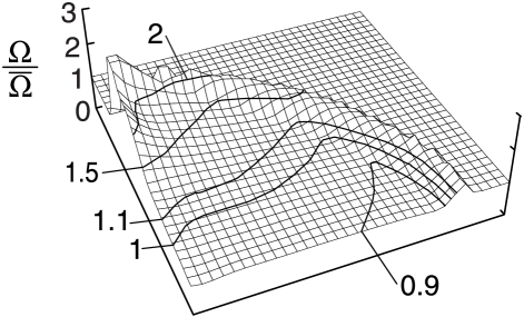
Figure 14: Meridional structure of the differential rotation in production run C3. The plot shows the value of the azimuthally averaged angular velocity $\Omega(\varpi,z)/\bar{\Omega}$, at time $t=25.6P_{0}$.

But we should not concentrate exclusively on the averaged quantity $\Delta\Omega/\bar{\Omega}$, which does not capture fully the spatial structure of differential rotation. Figure 14 illustrates the spatial dependence of the azimuthally averaged angular velocity,

$$\Omega(\varpi,z)=\frac{1}{2\pi}\int\Omega(\varpi,z,\varphi)\,d\varphi,$$ (30)

at the time when the amplitude is maximum, $t=25.6P_{0}$. The differential rotation is confined mostly to a thin shell of material near the surface of the star, and is particularly concentrated near each polar cap. The bulk of the material in the star remains fairly rigidly rotating.

V.6 Consistency of the radiation-reaction force

In these simulations we have assumed that the only relevant contribution to the radiation reaction force comes from the current quadrupole moment, and in particular from $J_{22}$. However, in the post-Newtonian approximation to general relativity, the lowest-order contribution to radiation reaction comes from the mass quadrupole term, followed by mass octupole and current quadrupole. To verify that our approximation is justified for the physical states considered here, we evaluate the additional energy that would have been lost to gravitational waves throughout our simulation if we had included the lowest-order mass multipole terms.

The mass multipole moments $Q_{lm}$ are defined by

$$Q_{lm}=\int\rho r^{l}Y^{*}_{lm}d^{3}x.$$ (31)

In the presence of density oscillations with sinusoidal dependences in the coordinates $t$ and $\varphi$ (i.e., $\delta\rho_{lm}\propto e^{i\omega_{lm}t+im\varphi}$) the flux of energy into gravitational waves is given by Thorne69 ; Ipser91

$$\left(\frac{dE}{dt}\right)_{Q_{2m}}\!\!\!\!\! = -\frac{8\pi}{75}\frac{G}{c^{5}}\omega_{2m}^{6}|Q_{2m}|^{2};$$ (32)

$$\left(\frac{dE}{dt}\right)_{Q_{3m}}\!\!\!\!\! = -\frac{8\pi}{6615}\frac{G}{c^{7}}\omega_{3m}^{8}|Q_{3m}|^{2}.$$ (33)

where $Q_{2m}$ and $Q_{3m}$ are, respectively, the mass quadrupole and mass octupole moments induced by these density fluctuations. Contributions of higher order are suppressed by very small fractional coefficients.

Comparing Eqs. (32) and (33) with Eq. (27) we find that the contribution of the density oscillations associated with the $r$-mode at frequency $\omega$ to the energy flux is negligible whenever

$$\frac{3c^{2}}{16}\frac{|Q_{2m}|^{2}}{|J_{2m}|^{2}}\ll 1,\quad\frac{5\omega^{2}}{2352}\frac{|Q_{3m}|^{2}}{|J_{2m}|^{2}}\ll 1.$$ (34)

We find that in our simulation both ratios are of order $10^{-3}$ before the $r$-mode saturates (at $t\simeq 25P_{0}$). The strongest contribution to the quadrupole term comes from $Q_{22}$, although the Fourier transform of this moment does not show any definite frequency of oscillation. The strongest contribution to the octupole term comes from the $Y_{32}$ dependence of the density in the $m=2$ $r$-mode (see the next subsection).

Between $t\simeq 25P_{0}$ and $t\simeq 32P_{0}$ (when $\alpha$ is back to its initial value $\approx 0.1$) the mass quadrupole term would have provided a correction of order 10% to the current quadrupole; although even then we see no evidence of a definite oscillation frequency correlated to the $r$-mode. Only after $t\simeq 32P_{0}$, when the fluid motion in the star becomes quite turbulent and the $r$-mode is very weak, is the gravitational radiation generated by the mass multipoles comparable to the radiation from $J_{22}$.

On the whole, we find that our approximation which ignores the contributions from the mass multipoles is well-justified throughout the more interesting part of the evolution.

V.7 Density oscillations and mode saturation

The evolution of the isodensity surfaces in our neutron star shows very clearly the presence of the lowest-order Eulerian density perturbation $\delta\rho$ associated with the $m=2$ $r$-mode. The lowest order expression for $\delta\rho$ was derived by Lindblom, Owen and Morsink Lindblom98 in the small-amplitude, slow-rotation approximation. Solving Eq. (5) of Ref. Lindblom98 with $m=2$ and with polytropic index $n=1$, and then substituting $\delta\Psi$ back into Eq. (4) of Ref. Lindblom98 , we get

$$\delta\rho=\alpha_{0}\frac{7\pi^{2}}{15}\sqrt{\frac{2}{3}}\frac{\Omega_{0}^{2}}{G}j_{3}\left({\pi r\over R_{0}}\right)Y_{32}(\theta,\varphi)e^{i\omega t},$$ (35)

where $j_{3}$ is the spherical Bessel function. The mass multipole associated with this $\delta\rho$ is

$$\delta Q_{32}=\alpha_{0}\frac{7\pi}{15}\sqrt{\frac{2}{3}}\frac{\Omega_{0}^{2}R_{0}^{5}}{G}j_{4}(\pi)Y_{32}(\theta,\varphi)e^{i\omega t},$$ (36)

where $j_{4}(\pi)=0.151425$.

We study the evolution of $Q_{32}$ throughout run C3. We find that $Q_{32}$ (and therefore the density perturbation with angular dependence given by $Y_{32}$) is indeed proportional to $\alpha$, at least as long as the growth of $\alpha$ remains exponential; after that, $Q_{32}$ grows more slowly than $\alpha$, and it reaches a maximum a few rotation periods before $\alpha$ (see Fig. 15). The phase evolution of the density perturbation is also consistent with expectations: the Fourier transform of $Q_{32}(t)$ shows a very definite peak at the $r$-mode (numerical) frequency $\omega$.

A quantitative check shows that Eq. (36) predicts the observed magnitude of $Q_{32}$ with an accuracy of about 50%; this error is consistent with the next-order terms ($\sim\Omega^{4}$ and $\alpha^{2}$) not included in this expression. In the slowly rotating calibration model C1, we find that $Q_{32}$ is given by Eq. (36) to within about 1%.

Figure 15: Numerical evolution of the mass moment $Q_{32}$ (solid line) and of the $r$-mode amplitude $\alpha$, in production run C3. The curve for $Q_{32}$ was renormalized to emphasize the linear relation between $\alpha$ and $Q_{32}$ during the growth of the $r$-mode.

We point out that we do not explicitly include any density perturbation in the initial configuration of the star; rather, the density perturbation is immediately generated by the hydrodynamic evolution of the fluid as a consequence of the initial velocity perturbation. The evolution of the amplitude of the density perturbation amplitude provides more insight into the mechanism that causes the $r$-mode to saturate: on the surface of the star, $\delta\rho$ appears as four large wave crests; at a critical amplitude these crests stop growing, and within a few rotation periods they turn into breaking waves that damp the $r$-mode.

V.8 Limits on mode–mode coupling

In the numerical evolution (C3) nonlinear hydrodynamic processes do not prevent the gravitational radiation instability from driving the dimensionless amplitude of the $r$-mode to values of order unity. In particular, the energy of the $r$-mode is not channeled into other modes by nonlinear hydrodynamic coupling until the amplitude of the mode becomes quite large. It is possible however that the nonlinear processes that would limit the growth of the $r$-mode act only on timescales that are longer than our artificially brief simulation growth time $\tau^{(s)}_{\mathrm{RR}}$, but still shorter than the physical $\tau^{(p)}_{\mathrm{RR}}$.

Can our numerical simulation place any limits at all on the possibility of nonlinear coupling? We know that in our simulation the amplitude of the $r$-mode grows exponentially until $\alpha\approx 2$, so the nonlinear interaction with other modes must be negligible at least until that time. This observation allows us to set a limit on the strength of the nonlinear couplings between the modes; and from this limit we can infer a lower limit on the saturation amplitude that may be achieved when the radiation-reaction coupling is adjusted to its physical value. Of course, the inference is only justified for the nonlinear interaction of the $r$-mode with other modes that are correctly modeled in our simulation (for instance, the finite azimuthal resolution of the grid sets an upper limit on the $m$ of the modes that can be resolved), and with our physical assumptions (for instance, the buoyant $g$-modes of realistic neutron stars will not be present with our choice of the equation of state).

Our argument is based on the Lagrangian description of the nonlinear evolution of the mode amplitude developed by Schenk, et al. Schenk01 . In this formalism, the modes interact at the lowest order by way of three-mode couplings: roughly speaking, quadratic interactions between pairs of modes drive the evolution of the amplitude of a third mode. Because at the beginning of our simulation all modes except the $r$-mode have negligible amplitude, we expect that the most important three-mode nonlinear term might be one that couples two $r$-modes to a third mode Schenk01 . Following Ref. Schenk01 we consider the coupled equations for the $r$-mode and a generic mode $X$ obtained in second-order Lagrangian perturbation theory:

$$\frac{dc_{R}}{dt}+i\omega_{R}c_{R} = \frac{c_{R}}{\tau_{\mathrm{RR}}}+\frac{i\omega_{R}}{2}\frac{\kappa^{*}_{XRR}}{\epsilon_{R}}c^{*}_{R}c^{*}_{X},$$ (37)

$$\frac{dc_{X}}{dt}+i\omega_{X}c_{X} = \frac{i\omega_{X}}{2}\frac{\kappa^{*}_{XRR}}{\epsilon_{X}}c^{*}_{R}c^{*}_{R},$$ (38)

where $c_{R}$ and $c_{X}$ are the complex amplitudes (including phases) of the modes; $\omega_{R}$ and $\omega_{X}$ are their frequencies; $\epsilon_{R}$ and $\epsilon_{X}$ are the nonlinear mode energies at unit amplitude; and $\tau_{\mathrm{RR}}$ is the radiation-reaction e-folding time of the $r$-mode. Finally, $\kappa^{*}_{XRR}$ is the nonlinear interaction energy for unit amplitude modes. Schenk, et al. Schenk01 give expressions for the $\kappa_{XRR}$ of coupled generic Newtonian modes in rotating stars. In writing Eqs. (37) and (38) we have omitted the coupling terms proportional to $\kappa^{*}_{XXR}$, which are forbidden by a $z$-parity selection rule Schenk01 : the $r$-mode has odd $z$ parity, so it cannot couple quadratically to the mode $X$.

From our numerical evolution C3, we know that the amplitude of the $r$-mode grows very nearly exponentially until $\alpha\simeq 2$:

$$c_{R}(t)\simeq c_{R}(0)e^{-i\omega_{R}t+t/\tau^{(s)}_{\mathrm{RR}}},$$ (39)

where $\tau^{(s)}_{\mathrm{RR}}$ is the artificially short radiation-reaction timescale used in our simulation. (Although it is convenient to take $|c_{R}|\simeq\alpha$, our argument still applies as long as $|c_{R}|$ is merely proportional to $\alpha$.) Therefore, we also know that until $|c_{R}|\simeq 2$, the second term on the right side of Eq. (37) is negligible compared to the first. In this case,

$${1\over\tau^{(s)}_{\mathrm{RR}}}\gg\left|\frac{i\omega_{R}}{2}\frac{\kappa^{*}_{XRR}}{\epsilon_{R}}c^{*}_{X}\right|.$$ (40)

We now use Eq. (39) to integrate Eq. (38) and compute $c_{X}$:

$$\!\!\!\!\!c_{X}(t) = c_{X}(0)e^{-i\omega_{X}t}$$ (41)

$$\!\!\!\!\!+\frac{i\omega_{X}}{2}\frac{\kappa^{*}_{XRR}}{\epsilon_{X}}\frac{[c_{R}^{*}(t)]^{2}-[c^{*}_{R}(0)]^{2}e^{-i\omega_{X}t}}{2i\omega_{R}+i\omega_{X}+2/\tau^{(s)}_{\mathrm{RR}}}.$$

Now we set $c_{X}(0)\simeq 0$ and $|c_{R}(t)|\gg|c_{R}(0)|$ for the time late in the simulation when $c_{R}\simeq 2$, and find

$$|c_{X}(t)|\simeq\left|\frac{\kappa^{*}_{XRR}}{\epsilon_{X}}\right|\frac{|\omega_{X}|\tau^{(s)}_{\mathrm{RR}}|c_{R}^{*}(t)|^{2}}{2\sqrt{\bigl{(}\tau^{(s)}_{\mathrm{RR}}\delta\omega\bigr{)}^{2}+4}},$$ (42)

where $\delta\omega\equiv 2\omega_{R}+\omega_{X}$. We define the resonance index $\gamma^{(s)}=|\omega_{R}/\omega_{X}|[(\tau_{\mathrm{RR}}^{(s)}\delta\omega)^{2}+4]^{1/2}$, whose value is close to unity, $\gamma^{(s)}\simeq 1$, when the system is near resonance, $\delta\omega\simeq 0$. We use this bound on $|c_{X}(t)|$ in Eq. (40) to obtain

$$\frac{1}{\tau^{(s)}_{\mathrm{RR}}}\gg\frac{|\kappa^{*}_{XRR}|^{2}}{4\epsilon_{X}\epsilon_{R}}\omega_{R}^{2}\tau^{(s)}_{\mathrm{RR}}\frac{|c_{R}^{*}(t)|^{2}}{{\gamma^{(s)}}}.$$ (43)

We can rewrite this inequality in terms of the $r$-mode period $P_{R}=2\pi/\omega_{R}$:

$$\left[\frac{P_{R}}{\tau^{(s)}_{\mathrm{RR}}}\right]^{2}\gg\pi^{2}\frac{|c_{R}(t)|^{2}}{{\gamma^{(s)}}}\left|\frac{\kappa^{*}_{XRR}}{\epsilon_{X}}\right|^{2}\frac{\epsilon_{X}}{\epsilon_{R}}.$$ (44)

We now set $|c_{R}(t)|=2$ (the value at which the evolution of the amplitude begins to show deviation from exponential) and $P_{R}/\tau^{(s)}_{\mathrm{RR}}=1/10$ (the value for our simulation), and obtain

$$\left|\frac{\kappa^{*}_{XRR}}{\epsilon_{X}}\right|^{2}\frac{\epsilon_{X}}{\epsilon_{R}}\ll\frac{\gamma^{(s)}}{400\pi^{2}}.$$ (45)

Thus, our numerical evolution puts a limit on the strength of the coupling between the $r$-mode and other modes in the star.

We now ask how the saturation amplitude would change if the radiation-reaction timescale assumed its physical value $\tau^{(p)}_{\mathrm{RR}}$ instead of the value $\tau^{(s)}_{\mathrm{RR}}$ used in our simulation C3. The key to doing this is to realize that Eqs. (37) and (38) describe the coupled mode evolution in the physical case if we just substitute $\tau^{(p)}_{\mathrm{RR}}$ for $\tau^{(s)}_{\mathrm{RR}}$. The mode $X$ is capable of stopping the unstable growth of the $r$-mode only when the magnitude of the second term on the right side of Eq. (37) becomes comparable to the first. Through an analysis similar to the one that led to Eq. (44), it is straightforward to find the following condition on the saturation amplitude of the $r$-mode,

$$\left[\frac{P_{R}}{\tau^{(p)}_{\mathrm{RR}}}\right]^{2}\simeq\pi^{2}\frac{|c_{R}^{\mathrm{sat}}|^{2}}{\gamma^{(p)}}\left|\frac{\kappa^{*}_{XRR}}{\epsilon_{X}}\right|^{2}\frac{\epsilon_{X}}{\epsilon_{R}}.$$ (46)

We now use the upper limit for $|\kappa^{*}_{XRR}|$ from Eq. (45) from our numerical evolution, to obtain a lower limit for the amplitude $c^{\mathrm{sat}}_{R}$ at which the $r$-mode would be saturated in the physical case:

$$|c^{\mathrm{sat}}_{R}|\gg 20\frac{P_{R}}{\tau^{(p)}_{\mathrm{RR}}}\sqrt{\frac{\gamma^{(p)}}{\gamma^{(s)}}}.$$ (47)

Since $\gamma^{(p)}>\gamma^{(s)}$ this equation yields $|c_{R}^{\mathrm{sat}}|\gg 4\times 10^{-4}$ for run C3. So if the dominant mode–mode coupling is of the form given in Eqs. (37) and (38), our simulation places a relatively large lower limit on the $r$-mode saturation amplitude. However, the $r$-mode could instead be limited by parametric resonance Dziembowski85 with a suitable pair of modes (satisfying the resonance condition $\omega_{R}+\omega_{Y}+\omega_{Z}\simeq 0$). It appears that our simulation does not provide a very strong lower limit on the saturation amplitude that could be imposed by this kind of process.

V.9 Dependence on the grid spacing

We wish to confirm that our standard computational grid can resolve the spatial structure of the $r$-mode well enough to give reliable predictions about the saturation amplitude of the mode. For this purpose, we have performed a simulation (run C3*) with the same parameters of run C3, but on a grid with only half the spatial resolution (i. e., 32 cells in the radial direction, and 64 cells in the axial and azimuthal directions). Figure 16 compares the evolution of $\alpha$ in runs C3 and C3*. The two curves are very similar, but in run C3* saturation is reached a bit earlier, at $t/P_{0}=21.4$, and at a somewhat lower amplitude $\alpha=2.68$. This may be caused by the larger numerical viscosity that must be present in the coarser grid. The evolution of the other diagnostics is also very similar in the two runs.

Figure 16: Numerical evolution of the $r$-mode amplitude $\alpha$ in low-resolution run C3* (solid curve) and in run C3 (dashed curve).

Thus, the simulation run (C3*) suggests that the qualitative results of our simulations are independent of the resolution adopted. The $r$-mode saturation amplitudes on the two grids agree to within about 20%. Interestingly, the extrapolation to the infinite resolution case suggests that the physical saturation amplitude might be even larger than 3.3.

VI testing the saturation amplitude

Even in the absence of a saturation mechanism due to mode–mode coupling as described above, it is possible that the saturation amplitude in our simulation might still depend on the strength of the radiation-reaction force. In our simulation we see that the $r$-mode grows until density waves on the surface of the star break and form shocks. It is possible that this occurs just because in our simulation we are pushing the fluid too hard with the radiation-reaction force, much harder than it would be appropriate in the physical case. To explore how the evolution depends on the strength of this driving force, we go back to the time in run C3 before any signs of nonlinear saturation are seen, when $\alpha=1.8$. We start a new run (C4) there, increasing the value of $\kappa$ (which determines the strength of the radiation-reaction force) to 5967 (1.33 times its value in run C3). The new growth timescale is about $7.5P_{0}$. (Undoubtedly, a test with $\kappa\ll 4487$ would have been more compelling; but our evolutions are so computationally expensive that we were forced to increase rather than decrease the strength of the driving force.)

In a separate run (C5), we test the influence of the history of the evolution of the $r$-mode on its saturation amplitude. Namely, we ask if an $r$-mode that started out as the linear initial data of Eq. (23), with a very large amplitude, would evolve much differently from an $r$-mode that started out small and was built up gradually to large amplitude by the radiation reaction force. To answer this question, we start with the Fast equilibrium model, and we add a linear $r$-mode velocity field with $\alpha_{0}=1.8$. For this run we keep $\kappa=4497$.

Figure 17: Numerical evolution of the $r$-mode amplitude $\alpha$ in production runs C3–C5.

Figure 18: Numerical evolution of the $r$-mode frequency $\omega$ in production runs C3–C5.

Figures 17, 18, and 19 show the evolution of the diagnostic parameters $\alpha$, $\omega$ and $\Delta\Omega$ for runs C3–C5. As expected, the $r$-mode does grow faster in run C4, but its maximum value is essentially the same (the maximum $\alpha=3.338$ at $t=24.12P_{0}$) as in run C3. In this run, the $r$-mode amplitude increases from $\alpha=1.8$ to $\alpha=3.338$ within a time $\Delta t\simeq 6P_{0}$ (compared to $\Delta t\simeq 8P_{0}$ in run C3) as would be expected given that the driving force is $\frac{4}{3}$ times that of run C3.

In run C5, the growth of the $r$-mode is initially slower than in run C3, as the linear $r$-mode velocity field evolves toward its correct nonlinear form. Eventually its maximum occurs at essentially the same amplitude as before ($\alpha=3.337$). Figures 17 and 18 show that during run C5 $\alpha$ and $\omega$ undergo short-period oscillations; this happens because the initial velocity field is only a small-amplitude approximation to the real $m=2$ $r$-mode eigenfunction. So other spurious modes with fairly large amplitude are excited initially in run C5. Note that these extraneous modes must make nonzero contributions to $J_{22}$ if they are to show up in our diagnostics. Here the extraneous modes cause a rapid modulation of $\alpha$ and $\omega$ with a dominant period of about $0.5P_{0}$. Finally, it is interesting to consider the evolution of $\Delta\Omega$ (Fig. 19), which is very similar in the three runs.

Figure 19: Numerical evolution of the differential rotation $\Delta\Omega$ in production runs C3–C5.

These runs provide limited evidence that the saturation amplitude of the $r$-mode does not depend (strongly) on our artificially large radiation reaction force. The nonlinear hydrodynamical process that leads to shock formation appears to be triggered by attaining a certain critical amplitude of the $r$-mode, with little dependence on the strength of the radiation-reaction force. Thus if no mode–mode coupling occurs on timescales longer than our unphysically short $\tau^{(s)}_{RR}$, then our results suggest that the maximum amplitude $\alpha\approx 3$ is a reasonable guess for the physical case ($\kappa=1$) as well.

VII Free evolution

Stergioulas and Font Stergioulas01 have also studied the nonlinear evolution of $r$-mode initial data, but using relativistic hydrodynamics in a fixed background geometry. In their evolution using this relativistic Cowling approximation, the gravitational interactions of the mode with itself and with the rest of the star are neglected. The principal difference between their model and ours therefore is that theirs has no radiation reaction, and no $r$-mode growth.

Stergioulas and Font find that, for an initial $r$-mode amplitude $\alpha_{0}=1.0$, no significant suppression of the mode is observed during 13 rotation periods. They define their mode amplitude using a post-Newtonian expression for the eigenfunction that differs from our Eq. (23) except in the Newtonian limit. And their method of evaluating the mode amplitude numerically also differs from ours. They read the mode amplitude from the value of the fluid’s velocity at a single point within the star, while we define $\alpha$ in terms of integrals over the entire star. In the slow-rotation Newtonian limit our two definitions agree. Stergioulas and Font observe that the amplitude of the velocity oscillations (shown in Fig. 2 of Ref. Stergioulas01 ) decrease by about 50% during the course of their simulation, an effect that they attribute to numerical viscosity Stergioulas01 . In order to compare our own simulations more directly with theirs, we performed a series of evolutions in which we turned off the radiation-reaction force by setting $\kappa=0$.

In production runs C6 and C7, we augment our rapidly rotating equilibrium configuration with the approximate $r$-mode velocity field of Eq. (23). For run C6, we choose the initial $\alpha_{0}$ so that $\alpha$ [as measured by our numerical diagnostic, Eq. (9)] is initially 1.8: the value at which we start to observe deviations from exponential growth in run C3. For run C7, we choose $\alpha_{0}$ so that the initial $\alpha$ is 1.0, in order to make a direct comparison with Stergioulas’ and Font’s published results. We have evolved these systems through respectively 11 and 7 initial rotation periods (several hydrodynamical timescales, according to our rough estimate of the speed of sound for the rapidly rotating model).

Figure 20: Numerical evolution of the $r$-mode amplitude $\alpha$ in production runs C6–C8.

We plot the evolution of $\alpha$ and $\omega$ for these simulations in Figs. 20 and 21. The wavy appearance of the curves suggests that, by using the linear eigenfunction, Eq. (23), for amplitudes of order unity, we have excited spurious modes in addition to the basic $m=2$ $r$-mode. We have already observed this behavior in run C5. The rapid modulation of $\alpha$ and $\omega$ has a period of about $0.5P_{0}$, and the amplitude of the modulation is smaller for run C7. (This is reasonable: for lower $\alpha$ we expect the approximate expression, Eq. (23), to be more accurate and so to excite smaller amplitude spurious modes.)

Figure 21: Numerical evolution of the $r$-mode frequency $\omega$ in production runs C6 and C7.

In both runs, $\alpha$ loses about 20% of its initial value during the first four rotation periods. In the next few rotation periods, however, the average value of $\alpha$ remains unchanged (although in run C6 we can see a further modulation of the amplitude with a period of about $8P_{0}$). Throughout the runs, the $r$-mode frequency $\omega$ oscillates around $\omega=-1.12\Omega_{0}$, consistent with its value in run C3 for the same value of $\alpha$ (i. e., 1.44). As the run is started, the differential rotation $\Delta\Omega$ (which is zero in the initial, rigidly rotating star) increases almost immediately to values that are consistent with those observed in run C3 for the same amplitude; compare Figs. 22 and 13. As $\alpha$ decreases, $\Delta\Omega$ decreases consistently. (In run C7, $\Delta\Omega$ settles to a value slightly higher than what we expected from its value in run C3 when $\alpha=0.82$; but we did not run this evolution as far as run C6, so at the end of our simulation the value of $\Delta\Omega$ might still be evolving.)

Figure 22: Numerical evolution of the differential rotation $\Delta\Omega$ in production runs C6–C8.

Finally, we study the free nonlinear evolution of an $r$-mode that was grown to the amplitude $\alpha=1$. To do so, we go back to the time in run C3 when $\alpha=1$, and start a new run (C8) using the C3 data at this time. We evolve these data setting $\kappa$ to zero in the subsequent evolution. We follow this evolution through an additional 15.4 initial rotation periods. During this time the mode amplitude $\alpha$ is essentially constant, see Fig. 20, except for a slow secular decline due to numerical viscosity at 0.23%/revolution, and a few very small amplitude oscillations. The $r$-mode frequency is quite constant, and the phase coherence function, and the differential rotation $\Delta\Omega$ also remain quite small in this case (see Fig. 22). The $r$-mode amplitude in run C3 remains above unity for 14.3 rotation periods, so run C8 demonstrates that the LSU hydrodynamic code Tohline97 ; Tohline01 used here reliably and stably evolves large amplitude $r$-modes in rapidly rotating stars for the duration of our simulations.

Comparing runs C6, C7, and C8, we infer that the strong decrease in the amplitude observed in runs C6 and C7 occurs as nonlinear hydrodynamics reorganizes the initial linear $r$-mode velocity field to the correct nonlinear form for amplitudes of order unity. After the reorganization is complete (within a few rotation periods), $\alpha$ decreases only because of numerical viscosity. (In run C5, this same phenomenon caused the slower growth of the amplitude compared to run C3.) By contrast, the small decrease in run C8 appears to be caused entirely by numerical viscosity.

Altogether, we find that our results are compatible with those of Stergioulas and Font Stergioulas01 : no nonlinear saturation effect is evident in the free nonlinear evolution of $r$-modes, at least for amplitudes of order unity.

VIII repeated spindown episodes?

The first attempt to analyze the nonlinear evolution of $r$-modes by Owen, et al. Owen98 was based on a simple two-parameter model consisting of a rotating star with angular velocity $\Omega$ and its $r$-mode with amplitude $\alpha$. Using this model the mode was found to grow exponentially until it reached some maximum level $\alpha_{\mathrm{max}}$, where it was assumed to remain saturated. Energy and angular momentum were expected to be removed from the star by gravitational radiation during this saturation phase until the $r$-mode regained stability (because of increased internal dissipation brought about by cooling or because the angular momentum of the star was reduced to a very low level). In this initial picture gravitational radiation was expected to spin down the star on a timescale of about one year. The radiation emitted was expected to sweep down in frequency from $\frac{4}{3}$ times the initial angular velocity of the star to $\frac{4}{3}$ times its final value: ranging from perhaps $1$ kHz initially to perhaps $100$ Hz.

Our simulations suggest a very different picture. We find that, once the amplitude of the $r$-mode reaches $\alpha_{\mathrm{max}}$, it is quickly reduced by the action of the breaking waves and shocks, instead of remaining saturated at this value for a very long time. At the end of our simulation the star still has 60% of its initial angular momentum, and its average angular velocity is 77.5% of $\Omega_{0}$. Thus the star is left rotating relatively rapidly, leaving open the possibility of subsequent episodes of $r$-mode instability and spindown.

To investigate this possibility, we extend run C4, evolving our star for 13 more initial rotation periods after $\alpha$ has gone back to its initial value (0.1), or (equivalently) for nine periods after $\alpha$ reaches its minimum ($\sim 0.01$). The evolution of the amplitude for this case is plotted in Fig. 23. After $t=33P_{0}$, the fluid motion is quite turbulent, but we see no sign that $\alpha$ is starting to grow again. The evolution of the $r$-mode frequency (Fig. 24) is also erratic, probably because here the sinusoidal approximation begins to fail (remember that $\omega$ is approximated as $-(1/J_{22})d|J_{22}|/dt$). In fact, after $t=33P_{0}$ we have found it necessary to impose an ad hoc limit on the value of $\omega$; otherwise $\omega$ grows to about $-17\Omega_{0}$, and the radiation-reaction force (proportional to $\omega^{6}$) becomes huge, pushing the fluid to superluminal velocities.

Figure 23: Numerical evolution of the $r$-mode amplitude $\alpha$ in the extended run C4.

Nine periods should be more than enough to see a second $r$-mode growth episode, if it occurs at all. Although at the end of the simulation the average angular velocity of the star is lower than $\Omega_{0}$, the growth timescale is determined by the $r$-mode frequency, which is even higher than at the beginning of the run. What keeps the $r$-mode then from resuming its growth?

Figure 24: Numerical evolution of the $r$-mode frequency $\omega$ in the extended run C4.

One hypothesis is that because of its strong differential rotation the post-spindown configuration of the star is one which stabilizes the $r$-mode. The value of $\Delta\Omega$ for the last few periods is plotted in Fig. 25. The increase of $\Delta\Omega$ observed between $t=32P_{0}$ and $t=36P_{0}$ is not caused by radiation reaction, but by a global, energy-conservative reorganization of the fluid. At the end of this process, the spatial structure of differential rotation is very different from what it was at $\alpha_{\mathrm{max}}$: compare Fig. 14 ($t=25.6P_{0}$ in run C3) with Fig. 26 ($t=42P_{0}$ in run C4). The latter plot shows a star that is rotating on cylinders (except for the outer layer), with $\Omega(\varpi,z)$ almost proportional to $\varpi$.

Figure 25: Differential rotation $\Delta\Omega$ through the extended run C4.

Karino, et al. Karino00 derived linearized structure equations for the $r$-modes of differentially rotating Newtonian stars. When differential rotation is so strong that corotation points appear (that is, when there exists a $\varpi$ such that $\omega+m\Omega(\varpi)=0$), the mode equations go singular. (The presence of a corotation point at the cylindrical radius $\varpi$ means that the velocity pattern of the mode appears to stand still in the frame rotating with angular velocity $\Omega(\varpi)$.) A comparison of the differential rotation of Fig. 26 with the value of $\omega$ suggests the presence of corotation points in the final configuration of our star. By itself, however, the singularity of the linearized mode equations does not necessarily mean that $r$-modes are impossible.

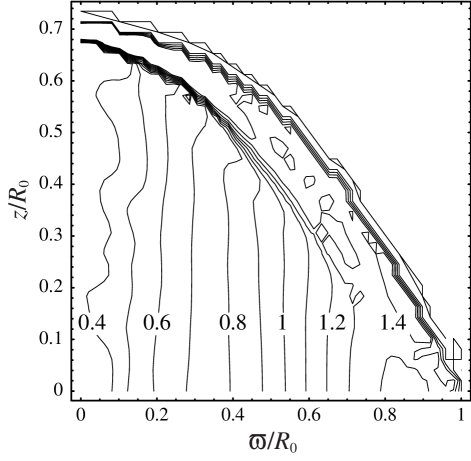
Figure 26: Meridional structure of differential rotation at the end of production run C4. This contour plot shows level contours for the value of the azimuthally averaged angular velocity $\Omega(\varpi,z)/\bar{\Omega}$, at time $t=42P_{0}$.

A second, probably more likely possibility is that, in the very noisy environment manifest in Figs. 23 and Figs. 24, the growing $r$-mode is unable to get locked in phase with the approximate expression for the driving force that we use here. The actual radiation reaction force [Eq. (17)] is a function of the frequency of the $r$-mode. Since we do not know exactly what this frequency is, we use the expression (11) to approximate it. This approximation works extremely well as long as the $r$-mode makes the dominant contribution to $J^{(1)}_{22}$; yet, in the turbulent post-spindown environment, the $r$-mode no longer dominates the evolution of $J_{22}$. Hence, our expression for the gravitational radiation reaction force is no longer correct: it fails to maintain phase coherence with the $r$-mode and so prevents the growth of the mode.

If the $r$-mode really does not exist in the chaotic post-spindown environment, then it will be necessary to wait for viscosity to damp differential rotation before the $r$-mode can grow again. However, viscosity might be unable to do this before the star cools so much that the $r$-mode is stabilized (either because the star forms a crust or because viscosity itself has grown too strong). This possibility is worrisome, because the same environmental conditions (strong differential rotation and generalized noise) that characterize the end of run C4 are likely to occur in the young supernova remnants where $r$-modes are expected to arise in nature. Still, we think it more likely that the absence of a second growth episode in our simulation is the result of our expression for the radiation reaction force, which is too simple for this chaotic situation.

IX Conclusions

We have completed a series of numerical 3D hydrodynamical simulations of the nonlinear evolution of the GR driven instability in the $r$-modes of rotating neutron stars. We have verified that the current-quadrupole GR reaction force implemented in our code is accurate by reproducing the analytical predictions (for slowly rotating stars) with our full 3D numerical integration code. In our simulations, the amplitude of the ($m=2$) $r$-mode is driven to a value of about three before nonlinear hydrodynamic forces stop its growth by the formation of shocks and breaking surface waves. We showed that the value of this maximum amplitude is insensitive to the strength of the GR driving force by repeating the simulation for different strengths and different initial fluid configurations. We also repeated our simulation using a coarser numerical grid to verify the robustness of our results (the maximum mode amplitude changes only by about 20% when the number of grid points is reduced by a factor of 8), and to show in particular that numerical viscosity is not playing a critical role in our simulations.

In our simulation we have artificially increased the strength of the GR reaction force in order to reduce the problem to one that can be studied with the available computer resources. We have shown, however, that the results of our simulation can be used to infer limits on the real physical problem as well. We used the results of our simulations to derive a lower limit of a few times $10^{-4}$ on the saturation amplitude of the $r$-mode in a real neutron star due to possible (but unseen) nonlinear mode–mode couplings. This lower limit applies to couplings with modes that are well described by our simulation: that is, the modes of a barotropic fluid with spatial structures larger than about 2% of the radius of the star.

Recent analysis of the effects of magnetic fields Rezzolla01 , and exotic forms of bulk viscosity Lindblom01b suggest that the $r$-mode instability may not play as important a role in astrophysical situations as was once thought. However, the considerable uncertainty that exists about both the macroscopic and microscopic states of a neutron star makes it impossible at the present time to conclude that the $r$-mode instability plays no astrophysical role. Thus it seems reasonable to us that some effort be put into gravitational wave searches for $r$-mode signals having forms qualitatively similar to those predicted by simulations such as this.

*

Appendix A Useful expressions in cylindrical coordinates

In this Appendix we give explicit expressions in cylindrical coordinates $(\varpi,z,\varphi)$ for a number of useful quantities used in our simulations. The components of the the initial $r$-mode velocity field used in our numerical evolutions are

$$v^{\varpi}=\alpha_{0}\sqrt{\frac{5}{16\pi}}\frac{\Omega_{0}}{R}z\varpi\sin 2\varphi,$$ (48)

$$v^{z}=-\alpha_{0}\sqrt{\frac{5}{16\pi}}\frac{\Omega_{0}}{R}\varpi^{2}\sin 2\varphi,$$ (49)

and

$$v^{\hat{\varphi}}=\Omega_{0}\varpi+\alpha_{0}\sqrt{\frac{5}{16\pi}}\frac{\Omega_{0}}{R}z\varpi\cos 2\varphi.$$ (50)

We refer the azimuthal component of the velocity to the orthonormal coordinate $\hat{\varphi}$, so that $v^{\hat{\varphi}}$ and $v_{\hat{\varphi}}$ have the same numerical value and we can use them interchangeably.

The integrals that determine $J_{22}$ and its first time-derivative $J^{(1)}_{22}$ are,

$$J_{22}=\sqrt{\frac{5}{16\pi}}\int\rho e^{-2i\varphi}[zv_{\hat{\varphi}}+i(zv_{\varpi}-\varpi v_{z})]\varpi^{2}d\varpi dzd\varphi,$$ (51)

and

$$J^{(1)}_{22}=\sqrt{\frac{5}{16\pi}}\int\rho e^{-2i\varphi}[T_{1}+iT_{2}]\varpi d\varpi dzd\varphi,$$ (52)

where

$$T_{1} \equiv 2zv_{\varpi}v_{\hat{\varphi}}-\varpi v_{z}v_{\hat{\varphi}}-z\frac{\partial\Phi}{\partial\varphi},$$ (53)

$$T_{2} \equiv z(v^{2}_{\varpi}-v^{2}_{\hat{\varphi}})-\varpi v_{\varpi}v_{z}+\varpi^{2}\frac{\partial\Phi}{\partial z}-z\varpi\frac{\partial\Phi}{\partial\varpi}.$$ (54)

The components of the radiation-reaction force in cylindrical coordinates are obtained from Eq. (17) by expressing the current multipole tensor $S_{jk}$ in terms of the current multipole moments $J_{2m}$ via Eqs. (19)–(21):

$$F^{\mathrm{GR}}_{z} = -\kappa\frac{16}{45}\sqrt{\frac{4\pi}{5}}\frac{G}{c^{7}}\rho\varpi$$

$$\times{\mathrm{Im}}\biggl{\{}e^{2i\varphi}\Bigl{[}3(v_{\varpi}+iv_{\hat{\varphi}})J^{(5)}_{22}+\varpi J^{(6)}_{22}\Bigr{]}\biggr{\}},$$

and

$$F^{\mathrm{GR}}_{\hat{\varphi}}-iF^{\mathrm{GR}}_{\varpi}=\kappa\frac{16}{45}\sqrt{\frac{4\pi}{5}}\frac{G}{c^{7}}\rho\varpi\,e^{2i\varphi}\Bigl{[}3v_{z}J^{(5)}_{22}+zJ^{(6)}_{22}\Bigr{]},$$ (56)

where $\kappa=1$ in general relativity theory. The fifth and sixth time derivatives of $J_{22}$ are obtained as $J^{(5)}_{22}=\omega^{4}J^{(1)}_{22}$, and $J^{(6)}_{22}=-\omega^{6}J_{22}$.

References

- (1) N. Andersson, Astrophys. J. 502, 708 (1998).
- (2) J. L. Friedman and S. M. Morsink, Astrophys. J. 502, 714 (1998).
- (3) L. Lindblom, B. J. Owen, and S. M. Morsink, Phys. Rev. Lett. 80, 4843 (1998).
- (4) L. Lindblom, and B. J. Owen, Phys. Rev. D(to be published).
- (5) B. J. Owen, L. Lindblom, C. Cutler, B. F. Schutz, A. Vecchio, and N. Andersson, Phys. Rev. D58, 084020 (1998).
- (6) L. Lindblom, J. Tohline, and M. Vallisneri, Phys. Rev. Lett. 86, 1152 (2001).
- (7) N. Stergioulas and J. A. Font, Phys. Rev. Lett. 86, 1148 (2001).
- (8) A. K. Schenk, P. Arras, É. É. Flanagan, S. A Teukolsky, and I. Wasserman, Phys. Rev. D65, 024001 (2002).
- (9) J. E. Tohline, “The Structure, Stability, and Dynamics of Self-Gravitating Systems” (work in progress), http://www.phys.lsu.edu/astro/H_Book.current/H_Book.shtml
- (10) K. C. B. New and J. E. Tohline, Astrophys. J. 490, 311 (1997); H. S. Cohl and J. E. Tohline, ibid. 527, 527 (1999); J. E. Cazes and J. E. Tohline, ibid. 532, 1051 (2000); P. Motl, J. E. Tohline, and J. Frank, Astrophys. J., Suppl. Ser. 138, 121 (2002).
- (11) J. M. Stone and M. L. Norman, Astrophys. J., Suppl. Ser. 80, 753 (1992).
- (12) J. Papaloizou and J. E. Pringle, Mon. Not. R. Astron. Soc. 182, 423 (1978).
- (13) L. Blanchet, Phys. Rev. D55, 714 (1997).
- (14) L. Rezzolla, M. Shibata, H. Asada, T. W. Baumgarte, and S. L. Shapiro, Astrophys. J. 525, 935 (1999).
- (15) I. Hachisu, Astrophys. J., Suppl. Ser. 61, 479 (1986); 62, 461 (1986).
- (16) S. Chandrasekhar, An Introduction to the Study of Stellar Structure (Dover, New York, 1967).
- (17) K. S. Thorne, Rev. Mod. Phys. 52, 299 (1980).
- (18) B. J. Owen, and L. Lindblom, Class. Quant. Grav. (to be published). eprint gr-qc/0111024
- (19) K. S. Thorne, Astrophys. J. 158, 997 (1969).
- (20) J. R. Ipser, and L. Lindblom, Astrophys. J. 373, 213 (1991).
- (21) W. Dziembowski, and M. Krolikowska, Acta Astron. 35, 5 (1985).
- (22) S. Karino, S. Yoshida, and Y. Eriguchi, Phys. Rev. D64, 024003 (2001).
- (23) L. Rezzolla, F. L. Lamb, D. Markovic, and S. L. Shapiro, Phys. Rev. D64, 104013 (2001); ibid. 64, 104014 (2001).