The Very Small Array

Abstract

The Very Small Array (VSA) is a fourteen-element interferometer designed to study the cosmic microwave background on angular scales of 2.4 to 0.2 degrees (angular multipoles $l$ = 150 to 1800). It operates at frequencies between 26 and 36 GHz, with a bandwidth of 1.5 GHz, and is situated at the Teide Observatory, Tenerife. The instrument also incorporates a single-baseline interferometer, with larger collecting area, operating simultaneously with and at the same frequency as the VSA main array. This provides accurate flux measurements of contaminating radio sources in the VSA observations. Since September 2000, the VSA has been making observations of primordial CMB fluctuations. We describe the instrument, observing strategy and current status of the first year of observations.

1 Introduction

	Compact Array	Extended Array
Mirror size /mm	143	322
Primary Beam (34 GHz)	4.6∘	2.0∘
Synthesised Beam (34 GHz)	$\sim$30′	$\sim$11′
$l$-range	150-700	300-1800
$\Delta$S (28$\times$7 hr) / mJy beam-1	30	6
$\Delta$T (28$\times$7 hr) / $\mu$K beam-1	33	33

Table 1: Basic VSA parameters

The Very Small Array (VSA) is a 14-element interferometer designed to make images of the cosmic microwave background (CMB) and to measure its power spectrum over angular scales of 2.4 to 0.2 degrees ($l$ = 150 to 1800). The telescope is located at the Teide Observatory, Tenerife at an altitude of 2400 m and, for observations in the region 26–36 GHz, the transparency at the site is approximately 98 percent. There is also negligible correlated emission from the atmosphere.

Interferometers are well-suited to measuring the power spectrum of the CMB since they directly sample the Fourier modes on the sky which can then be converted to a power spectrum. In addition they provide excellent rejection of systematics since only correlated signals are detected, reducing signals such as ground radiation and atmospheric emission. Interferometric systems also offer the opportunity to target a specific range of angular scales on the sky, determined by the spacing of the elements of the array.

In order to achieve constant temperature sensitivity over the full range of angular scales that the VSA is designed to measure, two separate, but scaled, array configurations are used. For measurement of the CMB power spectrum over $l$-values 150–700, a ‘compact array’ configuration is used. Each receiver is fitted with a 143 mm diameter antenna and typical baselines in this configuration range from approximately 30 cm to 120 cm. For mapping finer angular scales, the same receivers are re-fitted with larger antennas, 322 mm in diameter. The baselines of this ‘extended array’ are scaled by the same factor, thus allowing measurements to be made across the whole range of $l$ with constant temperature sensitivity. The specifications of these two arrays are given in Table 1.

The VSA project is a collaboration between the Cavendish Astrophysics Group, Cambridge, Jodrell Bank Obsevatory, Manchester, and the Instituto de Astrofisica de Canarias (IAC), Tenerife. Although the telescope can be operated remotely, on-site support is provided by the IAC. All three institutions are actively involved in the data analysis.

2 Design of the VSA

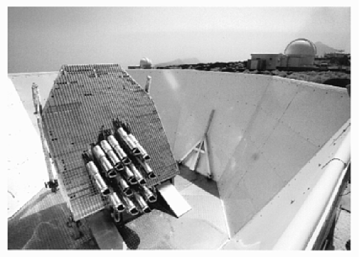
Figure 1: The VSA main array in its enclosure.

The basic design of the VSA is a development of the Cosmic Anisotropy Telescope (CAT) cat_inst , a three-element interferometer which operated at 15 GHz from a sea-level site in Cambridge. The VSA operates over the frequency range 26–36 GHz and has an observing bandwidth of 1.5 GHz. The front-end receivers are cryogenically cooled HEMT amplifiers and provide an overall system temperature of 25–35 K. Each receiver is fitted with a corrugated horn-reflector antenna in which the mirror can be rotated, providing tracking in one dimension. The fourteen VSA receivers are all mounted on a tip-table, providing pointing in a further dimension. Close packing of the array is achieved by mounting each element at 35^∘ to the table. The tracking range of the table in elevation is 0^∘–70^∘ resulting in a range of accessible declinations of $-7^{\circ}$ to $+63^{\circ}$. To eliminate ground radiation, the complete array is surrounded by a a 3.5 m high octagonal enclosure. Figure 1 shows the VSA main array in its enclosure.

Quasi-independent tracking of the VSA antennas is a key feature that distinguishes the VSA from other interferometric CMB experiments. Since each antenna tracks individually, the astronomical signal path to each antenna varies continuously during an observation. The rate of change of phase (or fringe rate) resulting from this continuous change in path can be calculated for each baseline configuration. The observed complex visibilities are then multiplied by the inverse of this expected fringe rate to give a quasi-constant signal. Since this is equivalent to applying a matched filter, all signals not varying at the expected fringe rate are removed. This rejection of systematics enables us not only to distinguish common systematics such as ground radiation or residual cross-talk between antenna elements but also to filter out the effects of bright sources such as the Sun and the Moon. We have been successful in removing the effects of both the Sun and Moon, even when they are as close as 30^∘ away from the VSA primary beam. The implementation and effectiveness of this filtering technique is discussed further by M. Jones in these proceedings.

A building alongside the main enclosure houses the VSA correlator and control room. The signal from each antenna is down-converted to 8.25–9.75 GHz on the table, with further down-conversion to baseband (0.25–1.75 GHz) before entering the control building. Phase-switching is provided at the first stage of down-conversion. Once inside a screened room, path compensation is provided, in increments of $\sim$ 7 mm, by a sequence of strip-line elements. Appropriate pairs of signals are then fed by a series of splitters to 182 correlators, providing the real and imaginary components of the correlated signal from each of the 91 baselines. The outputs of the correlator are sampled every second.

In addition to the VSA main array we operate a separate single-baseline interferometer, with much large collecting area, adjacent to the main enclosure. This 9-metre, north-south baseline operates simultaneously with and at the same frequency as the VSA, and forms part of our source-subtraction strategy described below.

3 Source Subtraction

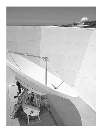
Figure 2: One of the 3.7m source-subtraction dishes.

Extragalactic radio sources are a major contaminant of CMB observations at centimetre wavelengths. Their population is not well known at frequencies higher than 10 GHz, and many are expected to be variable and/or have rising spectral indices, $\alpha$ (where S $\propto\nu^{-\alpha}$). On the angular scales of interest to primordial CMB work, such sources are also generally unresolved. We deal with this problem by observing all the contaminating radio sources in each VSA field at higher resolution than can be reached using the VSA. To achieve this, we implement a two-stage process.

First, prior to observation with the VSA, we survey all the VSA fields at 15 GHz using the Ryle Telescope (RT) in Cambridge. The RT, which uses five 13 m diameter antennas and gives a resolution of $\sim$30 arcsecs, is used in a raster scanning-mode and reaches an rms noise level of $\sigma$ = 4mJy waldram_iau . This allows us to identify all sources above 20 mJy at 15 GHz, and ensures that we find all sources above our source-confusion limit of 80 mJy at 34 GHz, even allowing for a spectral index as steep as $-$2 between 15 and 34 GHz.

Having identified the contaminating sources in each field, we monitor each source at 34 GHz using a separate single-baseline interferometer working simultaneously with the VSA. This single-baseline interferometer consists of two 3.7m dishes separated by 9 metres on a north-south baseline. Each dish is situated in an enclosure similar to that of the VSA (Fig. 2.) and is fitted with identical horn-reflector feeds and receivers as used on the main array. Every source identified in the 15 GHz survey is monitored daily and its contribution is subsequently subtracted in the $uv$ plane from VSA observations. The monitoring is done simultaneously with and at the same frequency as the VSA observation. This ensures that sources which are variable on time-scales as short as a few days can be subtracted accurately.

4 Observations

4.1 Field Selection

Figure 3: Plot of the VSA fields observed during our first year of observations. The hatched regions are fields which were observed using deep mosaicing. The remaining fields were observed as part of a shallow survey. Radio sources predicted to be brighter than 500 mJy are displayed as star symbols. A cut-off at galactic latitude b ¿ 20^∘ has been applied.

For practical CMB observation, it is important to choose fields which are relatively free from Galactic and extragalactic foregrounds. All the VSA fields are situated at Galactic latitudes greater than 20^∘ and have low Galactic synchrotron and free-free emission, as predicted by the 408-MHz all-sky radio survey of Haslam et. al. (1992)(408_mhz, ). The dust maps of Finkbeiner et. al. (1994) (dust, ) were used to select fields with relatively low dust contamination. To avoid large-scale structure and clusters we consulted the ROSAT catalogues (rosat, ),(xbacs, ). More importantly, all fields were chosen to be as free as possible of bright radio sources, since these are the major contaminant of CMB observations at 34 GHz. We used two low-frequency surveys, NVSS (nvss, ) at 1.4 GHz and Green Bank (gb6, ) at 4.85 GHz to select CMB fields in which there are predicted to be no sources brighter than 500 mJy at 34 GHz. Predictions were made by extrapolating the flux density of every source in the 4.8 GHz catalogue to 34 GHz on the basis of its spectral index between 1.4 and 15 GHz. A further practical consideration which affected the choice of CMB fields was the need to observe all fields for a reasonable length of time, from both Tenerife and Cambridge. This limited the declination range of our fields to +26^∘ – +54^∘. We also selected fields that are evenly spaced around the sky to enable 24-hour observing. In order to increase the $l$-resolution of our measurement of the CMB power spectrum, we selected regions of sky where we could mosaic several CMB fields. In each region of sky, mosaiced fields are separated by 2.75^∘. Our final choice of fields used during the first year of observation is shown in Fig. 3.

4.2 Observing strategy

During the first year of VSA observations, we have undertaken two distinct observation programs, each using a compact array. First, we have made deep mosaiced observations of eight fields in three evenly spaced regions of sky (hatched regions in Fig. 3.). Each mosaiced field was observed for $\sim$ 400 hours, reaching a thermal noise of approximately 30 mJy. Mosaicing in this way enables us to increase the $l$-resolution of our measurements whilst also reducing sample variance. However, the time taken for us to survey all fields with the Ryle Telescope prior to any observation with the VSA, has limited the area of sky that we can cover with deep mosaicing in this first year. Consequently, for $l$$\leq$ 300, our measurements of the CMB power spectrum are limited by sample variance. In order to achieve a good estimate of the CMB power spectrum in the region $l$$\leq$ 300, we have now completed the second stage of our observation program; a shallow survey in one area of sky. The shallow survey consists of 2 days observation on each of 30 mosaiced fields (Fig. 3 hexagonal region), and covers an area of approximately 180 sq. degrees. For this shallow survey, our source subtraction strategy no longer limits the area of sky we can observe with the VSA in a given time. Since we are only concerned with low-$l$ observations, where the contribution of point sources to the CMB power spectrum is known to be negligible, the need for prior surveying with the Ryle Telescope is not necessary. Instead, we choose only to monitor sources predicted to be greater than 100 mJy at 34 GHz on the basis of low-frequency survey information.

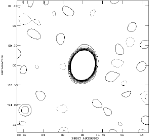
(a)        (b)

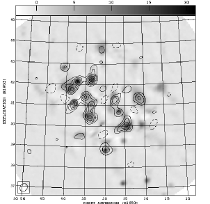
Figure 4: (a) An 80-minute observation of Jupiter, contoured at 0.3 Jy. The thermal noise level is 240 Jy (baseline $\times$ sec)^-1/2. (b) Commissioning observation of the Cygnus Loop. Contours (at 3 Jy) are VSA observations at 34 GHz. The grey scale is Green Bank, 4.85 GHz data cyg_loop .

4.3 Calibration

Absolute flux calibration of VSA observations is based on the flux scale of Mason et al. (1999) (mason_casscal, ). Flux calibrations are made each day using one of three primary calibrators – Tau A, Cass A and Jupiter. We also make daily observations of three fainter sources, 3C48, 3C273 and NGC7207 allowing us to check the quality of observations throughout the observing day. The measured flux ratios of these sources to our primary calibrators agree well with those reported by Mason et al., suggesting that the accuracy of our flux calibration is limited by that of Mason et al. to approximately 5 percent.

The overall gain of the telescope is also monitored via a noise injection system. A modulated noise signal is injected into each antenna and is later measured using phase-sensitive detection after the automatic gain control stage of the telescope. The relative contribution of the constant noise source to the total output power from each antenna varies inversely with system temperature, and thus a correction can be made to the overall flux calibration. This system allows us to account for both variations in the gain of the system and for atmospheric attenuation of the astronomical signal. It provides an excellent indication of the weather conditions and is used as a primary indicator for flagging data. For good observing conditions, the gain corrections applied using this system are typically less than a few percent.

Phase calibration of the VSA is also applied on a daily basis using the same three primary calibrators. We find that the VSA is relatively phase stable, with variations of less than 15 degrees per day. A typical calibration observation of Jupiter is shown in Fig. 4(a). This 80-minute observation, made early on in the observing program, also confirms that the telescope is achieving the required sensitivity, with a thermal noise level of approximately 240 Jy/(baseline$\times$sec)^1/2.

The pointing accuracy of the VSA is primarily determined by mechanical alignment tolerances, but we frequently make long observations of unresolved calibrators in order to check both the pointing and geometry of the array. Using these observations, and in conjunction with a model of the telescope, we employ a maximum-likelihood technique to simultaneously fit for $\sim$400 parameters. These include the $x$, $y$ and $z$ co-ordinate of each antenna, correlator gains for each of the 182 correlator channels and the effective observing bandwidth of each baseline. Further observations of offset sources and, for example, the Cygnus Loop, confirm the ability of the VSA to map known structure. Fig 4(b) shows the result of a 90-minute commissioning observation of the Cygnus Loop. Our observed 34 GHz flux contours are overlaid on 15 GHz Green Bank data cyg_loop . As shown in Fig. 4(b), there is good agreement between the structure observed at the two frequencies.

5 Current Status and Conclusions

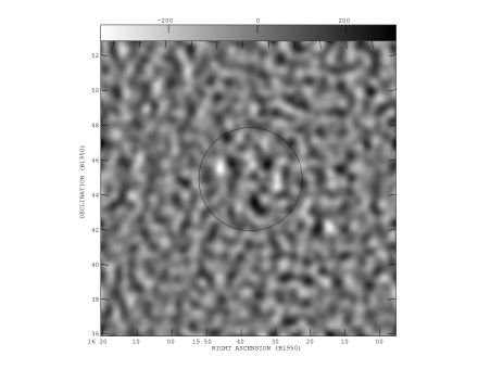
Figure 5: An example of a CMB field observed with the VSA. This map is the result of $\sim$ 400 hours of observation. The map has had a gaussian taper applied to enhance the CMB features present within the FWHM (black line) of the VSA primary beam.

The VSA has been making routine observations of CMB fields in its compact configuration since September 2000. Commissioning and calibration observations confirm that the instrument is working to specification. We have currently completed over 3000 hours of observations, having lost less than 10 percent of our observing time due to bad weather. A typical observation of one of our CMB fields is shown in Fig. 5. This map is the result of $\sim$ 400 hours of observation and, to enhance the CMB features present in the centre, a gaussian taper has been applied (1/e point = 60 $\lambda$). The resolution of the map is 31 $\times$ 25 arcmin. The map has not been source-subtracted.

Our observing program using the compact array was completed at the beginning of September 2001, and we are currently re-configuring and upgrading the array ready for observations in its extended configuration. The second season of observations with the new array will begin in October 2001. We will then be able to measure the CMB power spectrum for $l$-values up to $\sim$ 1800.

References

- (1) Robson, M., Yassin, G., Woan, G., Wilson, D. M. A., Scott, P. F., Lasenby, A. N., Kenderdine, S., and Duffett-Smith, P. J., A&A, 277, 314+ (1993).
- (2) Waldram, E. M., and Pooley, G. G., “Surveying the foreground sources for the VSA with the Ryle telescope at 15 GHz”, in IAU Symposium, in press, vol. 201.
- (3) Haslam, C. G. T., Stoffel, H., Salter, C. J., and Wilson, W. E., A&AS, 47, 1+ (1982).
- (4) Schlegel, D. J., Finkbeiner, D. P., and Davis, M., ApJ, 500, 525+ (1998).
- (5) Ebeling, H., Edge, A. C., Bohringer, H., Allen, S. W., Crawford, C. S., Fabian, A. C., Voges, W., and Huchra, J. P., MNRAS, 301, 881–914 (1998).
- (6) Ebeling, H., Voges, W., Bohringer, H., Edge, A. C., Huchra, J. P., and Briel, U. G., MNRAS, 281, 799–829 (1996).
- (7) Condon, J. J., Cotton, W. D., Greisen, E. W., Yin, Q. F., Perley, R. A., Taylor, G. B., and Broderick, J. J., AJ, 115, 1693–1716 (1998).
- (8) Gregory, P. C., Scott, W. K., Douglas, K., and Condon, J. J., ApJS, 103, 427+ (1996).
- (9) Langston, G., Minter, A., D’Addario, L., Eberhardt, K., Koski, K., and Zuber, J., AJ, 119, 2801–2827 (2000).
- (10) Mason, B. S., Leitch, E. M., Myers, S. T., Cartwright, J. K., and Readhead, A. C. S., AJ, 118, 2908–2918 (1999).