Reconnection in pulsar winds

Abstract

The spin-down power of a pulsar is thought to be carried away in an MHD wind in which, at least close to the star, the energy transport is dominated by Poynting flux. The pulsar drives a low-frequency wave in this wind, consisting of stripes of toroidal magnetic field of alternating polarity, propagating in a region around the equatorial plane. The current implied by this configuration falls off more slowly with radius than the number of charged particles available to carry it, so that the MHD picture must, at some point, fail. Recently, magnetic reconnection in such a structure has been shown to accelerate the wind significantly. This reduces the magnetic field in the comoving frame and, consequently, the required current, enabling the solution to extend to much larger radius. This scenario is discussed and, for the Crab Nebula, the range of validity of the MHD solution is compared with the radius at which the flow appears to terminate. For sufficiently high particle densities, it is shown that a low frequency entropy wave can propagate out to the termination point. In this case, the ‘termination shock’ itself must be responsible for dissipating the wave.
Dedicated to Don Melrose on his 60th birthday

1 Introduction

The supply of relativistic electrons and magnetic field needed to provide the synchrotron radiation observed from the Crab Nebula has long been thought to originate in a central star (Piddington 1957; Kardashev 1964). With the identification of this star as a pulsar, the earlier suggestion (Pacini 1967) that the star also emits a wave, whose energy is presumably released into the Nebula, attracted considerable attention (Ostriker & Gunn 1969; Rees & Gunn 1974). As an energy source for its environment, the Crab pulsar is by no means unique. The pulses of electromagnetic radiation emitted by other pulsars contain only a fraction of the power which the neutron star is apparently releasing from its store of rotational energy. In several cases, nebular emission is observed to surround the pulsar, but, even where it is not, it is generally thought that most of the spin-down power is carried away from the star by a relativistic wind consisting of a mixture of particles, waves and magnetic field. Attempts to provide a consistent description of this wind touch upon a fundamental problem in electrodynamics — the dichotomy between a single particle approach and a continuum description. In the pulsar wind case, one can either start from the solution describing a rotating magnetised object, compute individual particle trajectories and treat their combined effect as a perturbation, or, alternatively, consider the particles as a fluid and construct, for example, a solution with an ideal MHD wind emerging from a magnetised rotating star.

In the former case, it has been found that the wave component of the vacuum fields transfer energy rapidly to the particles. The resulting damping is strong and the wave will not propagate if the particle density exceeds a critical value (Asseo et al 1978; Leboeuf et al 1982; Melatos & Melrose 1996). Since the particle density decreases as the radius increases, the vacuum wave-like solution exists only outside a critical radius. In the fluid case, one faces the difficulty of formulating a generalised Ohm’s law. The simplest choice of infinite conductivity corresponds to ideal MHD, but has the problem that it may imply currents too large to be carried by the finite number of charged particles in the fluid. Given the structure of the magnetic field, the current densities can be computed from Ampère’s law. These generally decrease with radius less rapidly than the decrease in the density of charged particles available to carry the current (Usov 1975; Michel 1982). Since the velocity of the current carriers cannot exceed that of light, the MHD approach is valid only inside a critical radius. Thus, there are theoretical methods to describe both the inner and the outer parts of a pulsar driven wind. However, as yet, no way has been found of linking these two regimes.

In the case of the Crab Nebula, observations suggest that the wind energy is dissipated into relativistic particles at a radius $r\approx 10^{9}r_{\rm L}$, where $r_{\rm L}=c/\Omega$ is the radius of the light cylinder and $\Omega$ the angular velocity of the neutron star. The physics of this region (which we will term ‘termination shock’) is clearly an important problem. As a preliminary step, it is of interest to examine whether the wind solutions enable one to make a statement about the properties of the flow immediately before entering the shock region. This is the problem we address in this paper. We discuss a highly simplified non-axisymmetric ideal MHD wind — a ‘striped wind’ — and describe how a model of magnetic reconnection (Coroniti 1990; Michel 1994) modifies the wind dynamics (Lyubarsky & Kirk 2001, henceforth LK). As a result, the range of validity of the MHD solution is extended. Applying the results to the Crab pulsar wind, we find that for sufficiently high particle densities the solution is valid up to the location of the termination shock. We then speculate that the crucial physical process at work in the shock is the dissipation of the wave energy carried by the MHD wind.

2 The MHD wind

An exact analytic solution for an MHD pulsar wind has been found only for the idealised case of a monopole magnetic field in the force-free limit (Michel 1973). This solution has a very simple structure: the flow does not collimate, i.e., both the velocity and the magnetic field have purely radial components in the meridional plane, $B_{\theta}=0$, $v_{\theta}=0$ and there exist no closed field lines. A more realistic case would allow for closed field lines near the star, but, outside this region, it might be expected that the flow along open field lines mimics the monopole case, perhaps with a modified dependence on latitude. The obvious inconsistency of using a magnetic monopole as a source can be lifted by introducing the ‘split monopole’. In this case the system retains axial symmetry; the sign of each magnetic field component changes at the equator of the star, all other quantities remaining the same. A current sheet is then implied, which lies in the equatorial plane and separates the oppositely directed toroidal field components in the northern and southern hemispheres. It is also possible to lift the force-free approximation, replacing it by an ultra-relativistic approximation (Bogovalov 1997) to find that highly super-Alfvénic, relativistic winds also collimate only very slightly and the radial velocity pattern remains a good approximation, even when particle inertia is taken into account (Beskin et al 1998; Chiueh et al 1998; Bogovalov & Tsinganos 1999).

In a radial wind, the outward pressure gradient exerted by the magnetic field is precisely compensated by the inward tension force, so that the wind speed remains constant, as does the quantity $\sigma$, defined as the ratio of the Poynting flux to the energy flux in particles. Thus, a steady MHD wind driven by a magnetised neutron star carries energy predominantly in the form of Poynting flux, which is not converted into kinetic energy anywhere in the flow. This is a major difficulty, because modelling of the synchrotron emission of the Crab Nebula (Rees & Gunn 1974; Kennel & Coroniti 1984; Emmering & Chevalier 1987) suggests that if the wind terminates at a relativistic MHD shock, the energy flux must be carried predominantly by particles.

The rotating neutron star of a pulsar does not have an axisymmetric magnetic field, so that an axisymmetric wind is quite possibly a poor approximation. Non-axisymmetric solutions are, of course, very much more difficult to find. Fortunately, however, the technique of replacing a monopole source by a split monopole can also be used when the magnetic axis does not lie along the rotation axis (Bogovalov 1999). The solution is essentially the same as in the monopole case: the velocity field is unchanged, the pattern of the magnetic field lines is the same, but the direction (sign) of the field depends on the hemisphere in which the field line has its anchor point on the star. The current sheet, which lies in the equatorial plane in the axisymmetric case, takes on the form of an outward moving, spiral corrugation, as shown in Fig. 1.

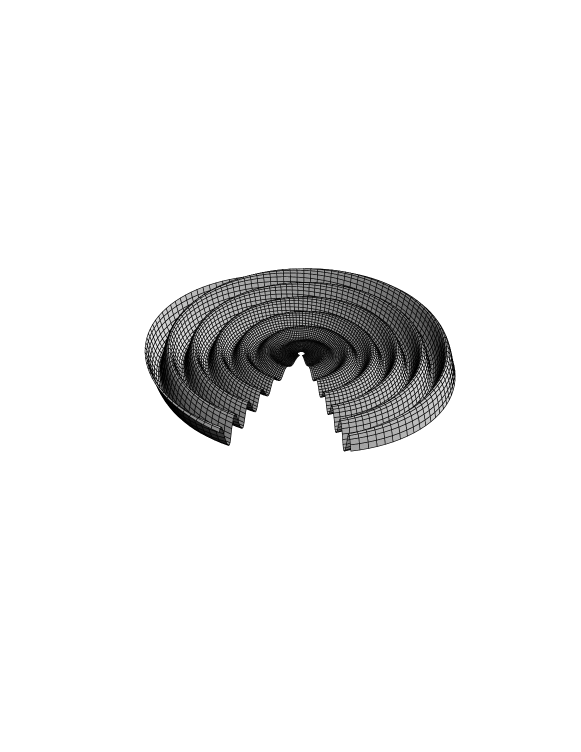
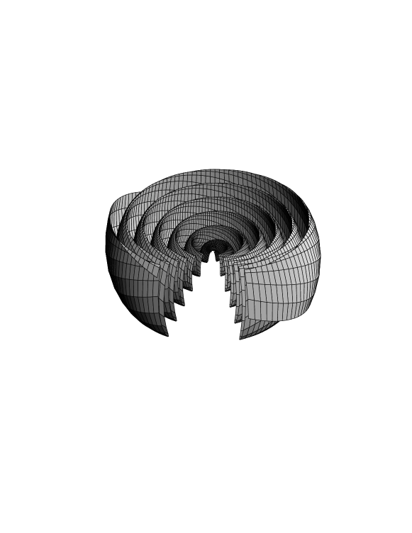
Figure 1: The current sheet in the split-monopole solution for a radial relativistic wind. The sheet has been truncated at a distance from the axis of $40r_{\rm L}$, and a sector has been removed for clarity. The wavelength of the corrugation is $2\pi r_{\rm L}$. The upper figure displays the sheet for an inclination angle $\chi$ between the rotation and magnetic axes of $6^{\rm o}$, the lower for an inclination angle of $26^{\rm o}$.

In the ultra-relativistic, highly super-Alfvénic limit, the solution in terms of spherical polar coordinates $(r,\theta,\phi)$ is given by:

$$\begin{array}[]{lll}u_{r}=\beta\gamma_{\rm L}&u_{\theta}=0&u_{\phi}=0\\ B_{r}=\pm B_{0}(r_{\rm L}/r)^{2}&B_{\theta}=0&B_{\phi}=\mp(r_{\rm L}\sin\theta/\beta r)B_{0}\\ E_{r}=0&E_{\theta}=\mp B_{0}\sin\theta(r_{\rm L}/r)&E_{\phi}=0\end{array}$$ (4)

(Bogovalov 1999), where $u_{r,\theta,\phi}$ are components of the four velocity, $B$ and $E$ are the magnetic and electric fields and $B_{0}$ is the magnitude of the radial component of ${\bf B}$ at the light cylinder, $r=r_{\rm L}$. The signs of $B_{r}$, $B_{\phi}$ and $E_{\theta}$ depend on whether the field line lies above (upper sign) or below (lower sign) the current sheet. Associated with this solution are distributed (‘body’) currents and charges as well as surface currents and charges located in the sheet. The body current is found from the curl of ${\bf B}$, (since the displacement current vanishes outside the sheet) and the body charge follows from Poisson’s equation:

$$\begin{array}[]{lll}j_{r}=-\left(cB_{0}\cos\theta/2\pi\beta r_{\rm L}\right)\left(r_{\rm L}/r\right)^{2}&j_{\theta}=0&j_{\phi}=0\\ \rho=\beta j_{r}/c\end{array}$$ (7)

The current sheet is located at the position $\Phi({\bf r})=0$, with

$$\Phi = \cos\chi\cos\theta+\sin\chi\sin\theta\cos\left({r-\beta ct\over\beta r_{\rm L}}+\phi\right)$$ (8)

where $\chi$ is the angle between the magnetic symmetry axis and the rotation axis and $\beta c\approx c$ is the 3-velocity of the wind. The surface current carried in the sheet is directed perpendicular to the adjacent magnetic field, and has the magnitude

$$k={c[1-\beta^{2}({\bf\hat{n}}\cdot{\bf\hat{r}})^{2}]\over 2\pi}\left|{\bf\hat{n}}\times{\bf B}\right|$$ (9)

where ${\bf\hat{n}}={\bf\nabla}\Phi/|{\bf\nabla}\Phi|$ is a unit vector normal to the sheet [e.g., Jackson (1975), pp 20–22]. Except at points where the sheet normal is perpendicular to ${\bf\hat{r}}$, the surface current scales with $1/r$, whereas the body current scales according to $j_{r}\propto 1/r^{2}$. The particle density in the wind drops off as $1/r^{2}$, so that the charge carriers can maintain the body currents without an increase in velocity. To maintain the surface currents, however, an increase with radius of either the surface density of charge carriers, or of their velocity is required. The MHD solution fails if equation (9) requires a current too large to be carried even if the particles contained in the sheet move at the speed of light.

3 Reconnection

At large radius, the corrugated current sheet described above resembles locally, a set of concentric nested spheres, when viewed at latitudes close to the equator ($|90^{\rm o}-\theta|\ll\chi$). The dynamics of the sheet may then be considered using a one-dimensional (radial) treatment. In the equatorial plane, the sheets of opposite polarity are evenly spaced. A sketch of the configuration at $r\gg r_{\rm L}$ is shown in Fig. 2.

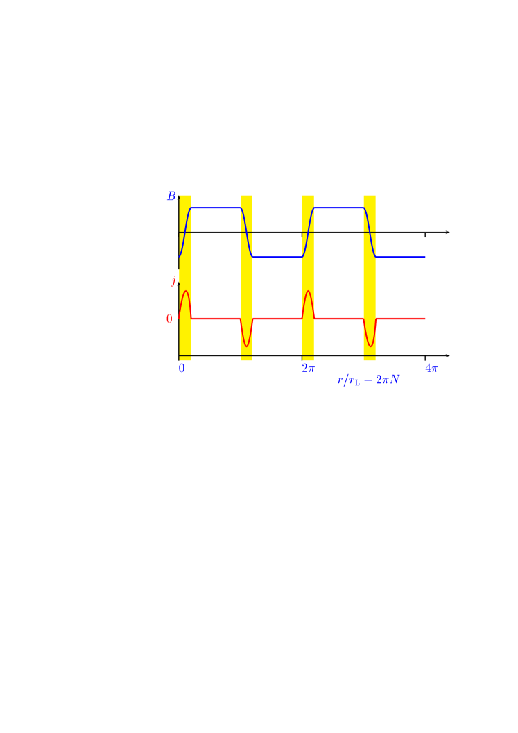
Figure 2: A schematic sketch of the radial structure of the magnetic field and current density in the wind far outside the light-cylinder ($N\gg 1$). In the equatorial plane, the current sheets are equally spaced, as shown. However, except in the singular case $\chi=90^{\rm o}$, the intersheet spacing depends on the magnetic polarity away from the equator and the sheets vanish altogether for $|90^{\rm o}-\theta|>\chi$

.

According to Ampère’s law, the integral of the current density across a current sheet is proportional to the change in magnetic field strength, measured in the comoving frame. In a radial wind, the toroidal field drops as $1/r$, and the particle density as $1/r^{2}$, when both quantities are measured in the lab. frame. Thus, in a wind of constant speed, the charge carriers in the sheet are forced to counter-stream with higher and higher velocities as the plasma moves outwards. This situation is likely to lead to instability, which could, in turn, provide an anomalous resistivity and hence magnetic reconnection. Coroniti (1990) [see also Michel (1994)] proposed a simple picture intended to capture the physics of magnetic reconnection in the sheets. The suggestion is that the sheets attain a minimum thickness equal to the gyro-radius which a particle in the hottest part of the sheet would have, if it were moving in the magnetic field adjacent to the sheets. Equivalently (to within a factor of order unity), the thickness can be set by demanding that the maximum current density in the sheets is equal to the product of the particle density, the electronic charge and the velocity of light. This enables one to formulate a system of equations for a wind that consists of two phases: a hot unmagnetised phase (corresponding to the current sheets) and a cold magnetised phase. From Fig. 1, it can be seen that, for an oblique rotator, the points at which a radius vector cuts the current sheet are equally spaced only in the equatorial plane. At other latitudes, the cold phase of one polarity dominates. In order to maintain pressure equilibrium, the magnetic field strength in the cold phase must remain constant on the scale of a wavelength, so that the cold phase of the dominant polarity is thicker than that of the opposite polarity. At a critical latitude ($\theta=90^{\rm o}-\chi$) the radius vector grazes the current sheet, and for $|90^{\rm o}-\theta|>\chi$ the hot phase is absent.

In Coroniti’s original work, the density in the hot and cold phases was assumed equal. However, this leads to inconsistencies and an incorrect picture of the evolution of the wind. Recently, Lyubarsky & Kirk (LK) have used a short wavelength approximation to analyse the evolution of the pattern of hot and cold phases, which is simply an entropy wave in the wind plasma. Reconnection at the sheet boundaries starts at a certain radius $r=r_{\rm start}$, which depends on how many particles are contained in the current sheet initially. The short wavelength approximation consists in assuming this radius to lie well outside the light-cylinder: $\varepsilon\equiv r_{\rm L}/r_{\rm start}\ll 1$. The slow evolution of the wave is governed by a set of five equations. Three of these are conveniently written in differential form. These are the conservation of particle number and of energy,

$${\partial\over\partial R}\left\{R^{2}\gamma_{0}v_{0}\left[\left(1-\Delta\right)n^{\prime}_{\rm c}+\Delta n^{\prime}_{\rm h}\right]\right\} = 0$$ (10)

$${\partial\over\partial R}\left\{R^{2}\gamma_{0}^{2}v_{0}mc^{2}\left[\left(1-\Delta\right)n^{\prime}_{\rm c}+\Delta n^{\prime}_{\rm h}\right]+2R^{2}\gamma_{0}^{2}v_{0}\left(1+\Delta\right){B^{\prime 2}\over 8\pi}\right\} = 0$$ (11)

and the entropy equation

$${4\Delta B^{\prime 2}\over R^{2}}{\partial\over\partial R}\left(R^{2}\gamma_{0}v_{0}\right)+3\gamma_{0}v_{0}{\partial\over\partial R}\left(\Delta B^{\prime 2}\right)+$$

$${v_{0}\over\gamma_{0}}{\partial\over\partial R}\left[\gamma_{0}^{2}\left(1-\Delta\right)B^{\prime 2}\right]+{2\gamma_{0}B^{\prime 2}\left(1-\Delta\right)\over R}{\partial\over\partial R}\left(Rv_{0}\right) = 0\enspace.$$ (12)

Here, $\gamma_{0}(R)$ and $v_{0}(R)$ are the zeroth order (in terms of $\varepsilon$) Lorentz factor and (3–)velocity of the flow, the dimensionless radius variable is $R=r/r_{\rm start}$, $\Delta(R)$ is the fraction of a wavelength occupied by the sheets, $n^{\prime}_{\rm c}(R)$ and $n^{\prime}_{\rm h}(R)$ are the (zeroth order) proper number densities in the cold and hot phases, respectively, and $B(R)=\gamma_{0}B^{\prime}(R)$ is the (zeroth order) magnetic field in the cold phase (the prime indicates a quantity measured in the plasma rest frame). The condition of ideal MHD (flux freezing) in the cold phase:

$${B\over rn_{\rm c}} = {\rm constant}$$ (13)

follows from the zeroth order equation of continuity, $r^{2}v_{0}n^{\prime}_{\rm c}={\rm constant}$ and the zeroth order Faraday equation, ${1\over r}{\partial\over\partial r}rE=-{1\over c}{\partial\over\partial t}B=0$ together with the ideal MHD condition $E=-vB$. The remaining equation stems from the requirement that the sheet thickness equal the gyro radius:

$$\Delta = {rn^{\prime}_{\rm c}c\over 4\pi n^{\prime}_{\rm h}\gamma_{0}v_{0}r_{\rm L}\kappa}$$ (14)

In this equation, we have introduced the multiplicity parameter $\kappa$, which is a dimensionless measure of the number density in the cold phase of the wind, in terms of the Goldreich-Julian density (see LK):

$$\kappa = {ecn_{\rm L}\over B_{\rm L}P}$$ (15)

where $P$ is the pulsar period, $n_{\rm L}=n_{i}/\varepsilon^{2}$ and $B_{\rm L}=B_{i}/\varepsilon$ are the density (in the cold phase) and magnetic field, extrapolated back to the light cylinder, in terms of the values $n_{i}$, $B_{i}$ at $r=r_{\rm start}$.

The set of differential equations (10), (11) and (12) together with (13) and (14) have been solved by LK. The solution is specified by three parameters, for example, the Lorentz factor $\gamma_{\rm L}$, the multiplicity $\kappa$ and the ratio of the particle gyro frequency $\omega_{\rm L}$ at $r=r_{\rm L}$ to the rotation frequency of the pulsar $\omega_{\rm L}/\Omega$. The values of the first two parameters are uncertain, but $\omega_{\rm L}/\Omega$ is more or less directly accessible from observation and is, to within a factor of a few, equal to the potential difference generated across open field lines, in units of the electron rest mass. (For the Crab pulsar $\omega_{\rm L}/\Omega\approx 10^{11}$.) As an alternative to the multiplicity, one may use the magnetisation parameter $\sigma_{\rm L}$, defined as the ratio at the light-cylinder of Poynting flux to particle energy flux in the cold phase of the wind, and related to the above parameters by $\sigma_{\rm L}=\omega_{\rm L}/(2\kappa\gamma_{\rm L}\Omega)$. In addition, the initial condition $r_{\rm rstart}$ must be given.

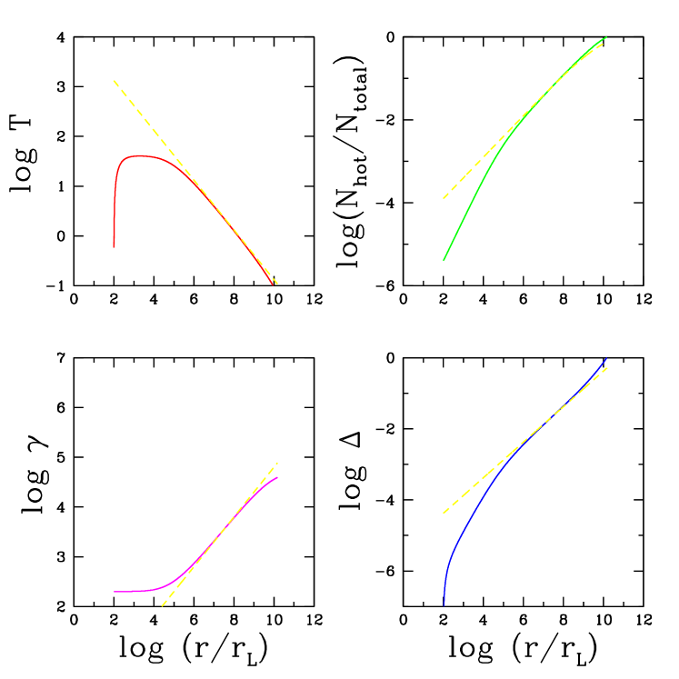
Figure 3: A numerical solution of the reconnecting striped wind problem, using parameters appropriate for the Crab pulsar: $\omega_{\rm L}/\Omega=10^{11}$, $\kappa=10^{5}$, $\gamma_{\rm L}=100$, corresponding to $\sigma_{\rm L}=5000$, and assuming reconnection starts at $r_{\rm start}=100r_{\rm L}$. The dashed line shows the asymptotic solution of LK.

In Fig. 3 we display an example of a solution appropriate for a pulsar that generates a maximum potential equal to that of the Crab pulsar: $\omega_{\rm L}/\Omega=10^{11}$. The multiplicity is chosen to be $\kappa=10^{5}$, and the initial Lorentz factor is $\gamma_{\rm L}=100$, (corresponding to $\sigma_{\rm L}=5000$). Reconnection is assumed to commence at $r_{\rm start}=100r_{\rm L}$, i.e., $\varepsilon=0.01$. As the magnetic flux is dissipated, the hot phase expands and performs work on the wind, causing it to accelerate. The system quickly approaches the asymptotic solution given by LK and shown as dashed lines. This solution reads:

$$\gamma = {1\over\kappa}\sqrt{\omega_{\rm L}r\over 8\pi\Omega r_{\rm L}}$$ (16)

$$\Delta = \sqrt{r\Omega\over 18\pi r_{\rm L}\omega_{\rm L}}$$ (17)

$${T^{\prime}\over mc^{2}} = \sqrt{\pi\omega_{\rm L}r_{\rm L}\over 18\Omega r}$$ (18)

$$p^{\prime} = 8\pi\left({B_{\rm L}^{2}\over 8\pi}\right)\left({r\over r_{\rm L}}\right)^{-3}\kappa^{2}\left({\omega_{\rm L}\over\Omega}\right)^{-1}$$ (19)

where $p^{\prime}=B^{\prime 2}/8\pi$ is the pressure of the hot phase and $T^{\prime}$ its temperature, in energy units.

4 Validity of the solution

The ideal MHD part of the solution, in which the radial velocity is constant and no magnetic flux is dissipated, is valid, by assumption, for $r<r_{\rm start}$. This range is determined by the surface density of charges assumed to be present in the quasi-spherical current sheets when they are first established. For $r<r_{\rm start}$ the current sheet contains a sufficient number of particles to supply the required current. Provided the initial surface density is small compared to the surface density of particles in the cold, magnetised phase (i.e., the integral of $n_{\rm h}$ over one wavelength) the sheets are able to maintain the required current at $r>r_{\rm start}$ by expanding and absorbing particles from the cold phase. In this way, the MHD picture of the wind retains validity, although the flow necessarily contains non-ideal regions in which oppositely directed magnetic flux is steadily annihilated. The solutions can be followed until the current sheets — as seen in the one-dimensional description — appear to merge. In the equatorial plane, this occurs at a radius given approximately by

$$r_{\rm max} \approx {\omega_{\rm L}\over\Omega}r_{\rm L}$$ (20)

and implies the complete annihilation of the magnetic field. Above and below the equatorial plane, the current sheets are not equally spaced, and the total magnetic flux passing through one complete wavelength of the pattern is non-zero. Since this flux is conserved in our picture, reconnection leaves behind a residual magnetic field, whose magnitude can be found from Eq. (8) and is

$$B_{\rm res} = {r_{\rm L}B_{\rm L}\over r}\left({2\arccos(\cot\chi\cot\theta)\over\pi}-1\right)$$ (21)

Beyond $r_{\rm max}$, the ‘current sheet’ is no longer corrugated, but lies in the equatorial plane. Since the toroidal magnetic field goes smoothly to zero as this plane is approached, the current it carries is proportional to the radial component of the field, which varies as $r^{-2}$. As in the axisymmetric, split-monopole case, the MHD picture is still valid, since the number of available particles is always sufficient to provide this current.

However, there are two limitations which restrict the validity of this solution at large radius. The first is the assumption, implicit in Eq. (14), that the electrons in the hot phase are relativistic. This is a relatively minor technical limitation of the treatment, which is encountered for radii more than a few percent of $r_{\rm max}$. The second limitation is more subtle, and can be stated in a number of ways. It also arises from Eq. (14). In prescribing the thickness of the sheet in terms of the densities in the two phases and the wind velocity, the movement of the sheet edge is decoupled from the local wave speeds, and can even move superluminally. Clearly, a physically realistic prescription would involve, at the very least, an additional dissipation of energy into waves when the velocity of the sheet edge approaches $c$. This point is reached when

$$v_{\rm edge} = v_{0}\left(1+{\pi r_{\rm L}\over 2}{{\rm d}\Delta\over{\rm d}r}\right)\,=\,c$$ (22)

which can be written, using Eq. (17)

$$\Delta = {2r\over\pi\gamma_{0}^{2}r_{\rm L}}$$ (23)

To within a factor of the order of unity, this is coincident with the limit discussed in LK [Eq. (36)]. Using the asymptotic solution, the critical distance $r_{\rm cr}$ beyond which the solution fails is

$$r_{\rm cr} = 1.5\times 10^{3}\kappa^{4}r_{\rm L}\left({\omega_{\rm L}\over\Omega}\right)^{-1}$$ (24)

Combining this with equation (20), we find

$${r_{\rm cr}\over r_{\rm max}} = 1.5\times 10^{3}\kappa^{4}\left({\omega_{\rm L}\over\Omega}\right)^{-2}$$ (25)

5 Discussion

The inclusion of non-ideal MHD effects — albeit phenomenologically — results in a substantial extension beyond $r_{\rm start}$ of the range of validity of the ‘inner’ wind solution, which can be described using a continuum picture. Starting with an entropy wave outside the light cylinder, this solution can exist up to a maximum radius $\sim r_{\rm max}$ (Eq. 20) and convert a substantial part of the total energy flux into bulk kinetic energy of the particles, provided $\kappa\,\raisebox{-1.72218pt}{$\stackrel{{\scriptstyle>}}{{\scriptstyle\sim}}$}\,0.1\sqrt{\omega_{\rm L}/\Omega}$ [see eq. (25)]. The situation in the outer parts of the wind then resembles the axisymmetric, split monopole solution, except that the magnitude of the toroidal component of the magnetic field passes smoothly through zero on crossing the equatorial plane. However, if $\kappa\,\raisebox{-1.72218pt}{$\stackrel{{\scriptstyle<}}{{\scriptstyle\sim}}$}\,0.1\sqrt{\omega_{\rm L}/\Omega}$, the solution loses validity at $r\sim r_{\rm cr}$ (Eq. 24) and the energy contained in the non-axisymmetric or (entropy) wave component must be channelled into another type of wave and/or into the particles.

In reality, the wind driven by a pulsar is confined by the surrounding medium, which may disrupt the solution either before reconnection is complete or before the MHD approach loses validity. Usually, disruption is envisaged to occur at a ‘termination shock’ where the flow makes an abrupt transition from supersonic to subsonic velocity. In the case of the Crab Nebula, this transition can be identified with a sharp increase in the synchrotron emissivity at a radius of approximately $r_{\rm shock}\equiv 10^{9}r_{\rm L}$. The Crab pulsar has $\omega_{\rm L}/\Omega=10^{11}$, so that, according to Eq. (20), $r_{\rm max}\gg r_{\rm shock}$ and very little of the striped magnetic flux has time to reconnect. For the MHD solution to remain valid up to $r_{\rm shock}$ a minimum number of particles is required. From Eq. (24) this may be expressed as a condition on the multiplicity parameter: $\kappa\,\raisebox{-1.72218pt}{$\stackrel{{\scriptstyle>}}{{\scriptstyle\sim}}$}\,1.6\times 10^{4}$. Assuming that this condition is satisfied, the region $r<r_{\rm shock}$ can be described by the striped MHD wind. Close to the equator, most of the energy flux is carried by the magnetic field of this entropy wave. If, in this region, the termination shock is to dissipate a substantial fraction of the wind energy, it must not only decelerate the wind to subsonic velocity, but also damp the oscillating component of the magnetic field. This conclusion is consistent with the constraints from modelling the synchrotron emission of the nebula, which indicate that the energy density of the plasma downstream of the shock is not dominated by the magnetic field. The physics of such a transition is at present unclear, but is likely to have profound implications for particle acceleration.

References

- Arons (1983) Arons J., 1983 in Electron-Positron Pairs in Astrophysics Eds. M.L. Burns, A.K. Harding, R. Ramaty (New York: American Institute of Physics), p. 163
- Asseo et al (1978) Asseo E., Kennel C.F., Pellat R. 1978 A&A 65, 401
- Beskin et al (1998) Beskin V.S., Kuznetsova I.V., Rafikov R.R., 1998 MNRAS 299, 341
- Bogovalov (1997) Bogovalov S.V., 1997 A&A 327, 662
- Bogovalov (1999) Bogovalov S.V., 1999 A&A 349, 1017
- Bogovalov & Tsinganos (1999) Bogovalov S.V., Tsinganos K. 1999 MNRAS 305, 211
- Chiueh et al (1998) Chiueh T., Li Z.Y., Begelman M.C., 1998 ApJ 505, 835
- Coroniti (1990) Coroniti F.V. 1990 ApJ 349, 538
- Emmering & Chevalier (1987) Emmering R.T., Chevalier R.A. 1987 ApJ 321, 334
- Jackson (1975) Jackson J.D. 1975 “Classical Electrodynamics” second edition, (John Wiley & Sons, New York), pp 20–22.
- Kardashev (1964) Kardashev N.S., 1964 Astron Zh. 41, 807 — translated in Sov. Astron. AJ 8, 643 (1965)
- Kennel & Coroniti (1984) Kennel C.F., Coroniti F.V., 1984 ApJ 283, 694
- Leboeuf et al (1982) Leboeuf J.N., Ashour-Abdalla M., Tajima T., Kennel C.F., Coroniti F.V., Dawson J.M., 1982 Phys. Rev. A25, 1023
- Lyubarsky & Kirk (2001) Lyubarsky Y.E., Kirk J.G. 2001 ApJ 547, 437 (“LK” in text)
- Melatos & Melrose (1996) Melatos A., Melrose D.B. 1996 MNRAS 279, 1168
- Michel (1973) Michel, F.C., 1973 ApJ Letts. 180, L133
- Michel (1982) Michel, F.C., 1982 Rev. Mod. Phys. 54, 1
- Michel (1994) Michel, F.C., 1994 ApJ 431, 397
- Ostriker & Gunn (1969) Ostriker J.P., Gunn J.E., 1969 ApJ 157, 1395
- Pacini (1967) Pacini F., 1967 Nature 216, 567
- Piddington (1957) Piddington J.H. 1957 Aust. J. Phys. 10, 530
- Rees & Gunn (1974) Rees M.J., Gunn J.E., 1974 MNRAS 167, 1
- Usov (1975) Usov V.V., 1975 Astrophys. & Space Sci. 32, 375