PINOCCHIO: pinpointing orbit-crossing collapsed hierarchical objects in a linear density field.

Abstract

PINOCCHIO (PINpointing Orbit-Crossing Collapsed Hierarchical Objects) is a new algorithm for identifying dark matter halos in a given numerical realisation of the linear density field in a hierarchical universe (Monaco et al. 2001). Mass elements are assumed to have collapsed after undergoing orbit crossing, as computed using perturbation theory. It is shown that Lagrangian perturbation theory, and in particular its ellipsoidal truncation, is able to predict accurately the collapse, in the orbit-crossing sense, of generic mass elements. Collapsed points are grouped into halos using an algorithm that mimics the hierarchical growth of structure through accretion and mergers. Some points that have undergone orbit crossing are assigned to the network of filaments and sheets that connects the halos; it is demonstrated that this network resembles closely that found in N-body simulations. The code generates a catalogue of dark matter halos with known mass, position, velocity, merging history and angular momentum. It is shown that the predictions of the code are very accurate when compared with the results of large $N$-body simulations that cover a range of cosmological models, box sizes and numerical resolutions. The mass function is recovered with an accuracy of better than 10 per cent in number density for halos with at least $30-50$ particles. A similar accuracy is reached in the estimate of the correlation length $r_{0}$. The good agreement is still valid on the object-by-object level, with 70-100 per cent of the objects with more than 50 particles in the simulations also identified by our algorithm. For these objects the masses are recovered with an error of 20-40 per cent, and positions and velocities with a root mean square error of $\sim$1-2 Mpc (0.5-2 grid lengths) and $\sim$100 km/s, respectively. The recovery of the angular momentum of halos is considerably noisier and accuracy at the statistical level is achieved only by introducing free parameters. The algorithm requires negligible computer time as compared with performing a numerical $N$-body simulation.

1 Introduction

In Dark Matter (DM) dominated cosmological models, structure grows through the gravitational amplification and collapse of small primordial perturbations, imprinted at very early times by some mechanism such as inflation. In particular in the case of Cold Dark Matter (CDM), the formation of structure follows a hierarchical pattern, with more massive halos forming from accretion of mass and mergers of smaller objects (see e.g. Padmanabhan 1993 for a general introduction). Galaxies form following the collapse of gas into these dark matter potential wells (see, e.g., White 1996 for a review). An accurate description of the non-linear evolution of perturbations in the DM field is thus important for modeling the formation and evolution of astrophysical objects within a cosmological setting.

The gravitational formation of dark matter halos is usually addressed by means of $N$-body simulations. However, a number of analytic or semi-analytic techniques based on Eulerian or Lagrangian perturbation theory (Bouchet 1997; Buchert 1997), for example the Press & Schechter (1974, PS) and similar techniques (see e.g. Monaco 1998 for a recent review), were devised to approximate some aspects of the gravitational problem. Analytic techniques have the advantage of being both fast and flexible, thereby giving insight into the dynamics of the gravitational collapse. In particular, Lagrangian Perturbation Theory (LPT; Moutarde et al. 1992; Buchert & Ehlers 1993; Catelan 1995) and more specifically its linear term, the Zel’dovich (1970) approximation, were used to compute many properties of the density and velocity fields in the ‘mildly non-linear regime’  when the density contrast is not very high, and particle trajectories still retain some memory of the initial conditions. The PS and extended PS approaches (Peacock & Heavens 1990; Bond et al. 1991; Lacey & Cole 1993) were used to generate merger histories of DM halos. Extensions of the PS approach to the non-linear regime were attempted by many authors (Cavaliere, Colafrancesco & Menci 1992; Monaco 1995, 1997a,b; Cavaliere, Menci & Tozzi 1996; Audit, Teyssier & Alimi 1997; Lee & Shandarin 1999; Sheth & Tormen 1999, 2001; Sheth, Mo & Tormen 2001). Alternative approaches assumed objects to form at the peaks of the linear density field (Peacock & Heavens 1985; Bardeen et al. 1986; Manrique & Salvador-Solè 1995; Bond & Myers 1996a,b; Hanami 1999), or applied the Zel’dovich approximation to smoothed initial conditions (truncated Zel’dovich approximation, Coles, Melott & Shandarin 1993; Borgani, Coles & Moscardini 1994), or used the second-order LPT solution for the density field (Scoccimarro & Sheth 2001), or joined linear-theory predictions with Monte-Carlo methods such as the block-model (Cole & Kaiser 1988) and merging-cell model (Rodrigues & Thomas 1996; Nagashima & Gouda 1998; Lanzoni, Mamon & Guiderdoni 2000).

These approaches are limited to the linear or mildly non-linear regime and are generally unable to recover accurately the wealth of information available with a large numerical simulation. In particular, although PS provides a reasonable first approximation to the mass function of halos (Efstathiou et al. 1988; Lacey & Cole 1994), it underestimates the number of massive objects and overestimates the number of low mass ones (see, e.g., Gelb & Bertschinger 1994; Governato et al. 1999; Jenkins et al. 2001; Bode et al. 2000). Similarly, the merger history of DM halos is reasonably well reproduced by the extended PS approach, but there are systematic differences when compared with simulations, and also some theoretical inconsistencies (Lacey & Cole 1993; Somerville & Kolatt 1999; Sheth & Lemson 1999). The clustering of halos of given mass in the PS approach can be obtained analytically (Mo & White 1996; Catelan et al. 1998; Porciani, Catelan & Lacey 1999; Sheth & Tormen 1999; Sheth et al. 2001; Colberg et al. 2001), but the extended PS approach is not able to produce both spatial information and merger histories at the same time. This is true also for many of the non-linear extensions of the PS approach mentioned above. The merging cell model can provide spatial information on the halos (Lanzoni et al. 2000), but only in the space of initial conditions (Lagrangian space), while the truncated Zel’dovich approximation, though able to predict correlation functions in the Eulerian space, is not accurate in predicting the masses of the single objects (Borgani et al. 1994). Finally, the peak-patch approach (Bond & Myers 1996a,b) can also generate catalogues of halos with spatial information, but has never been extended to predict the merging histories.

Semi-analytical models of galaxy formation assume that the properties of a galaxy depend on the merger history of its associated DM halo. So in order to make predictions of the clustering properties of galaxies of a given type, one needs to be able to compute the merger history and spatial clustering simultaneously. Given the limitations of the analytic techniques discussed above, such models have usually resorted to analysing large $N$-body simulations with very many snapshots to reconstruct the merger histories (see. e.g., Diaferio et al. 1999). Alternatively, the extended PS approach is used to compute the merger histories, but $N$-body simulations to obtain the spatial information on the halos statistically (e.g., Benson et al. 2000).

A new approach for obtaining the spatial information and the merger history simultaneously for many halos was recently proposed by Monaco et al. (2001, hereafter paper I; see also Monaco 1999 for preliminary results). In the PINOCCHIO (PINpointing Orbit-Crossing Collapsed HIerarchical Objects) formalism, LPT is used in the context of the extended PS approach, as in Monaco (1995; 1997a,b) and Monaco & Murante (1999), to provide predictions for the collapse of fluid elements in a given numerical realisation of a linear density field. Mass elements are assumed to have collapsed after undergoing orbit crossing. Such points are then grouped into halos using an algorithm that mimics the hierarchical growth of structure through accretion and mergers. The Zel’dovich approximation is used to compute the Eulerian positions of halos at a given time. Some points that have undergone orbit crossing are assigned to the network of filaments and sheets that connects the halos. Paper I contained a preliminary comparison to simulations, demonstrating that PINOCCHIO can accurately reproduce many properties of the DM halos from a large $N$-body simulations that started from the same initial density field. The good agreement is not only for statistical quantities such as the mass or the correlation function, but extends to the object-by-object comparison. PINOCCHIO thus provides a significant improvement over the extended PS approach, which is known to be approximately valid only in a statistical sense (Bond et al. 1991; White 1996).

In this paper, the PINOCCHIO code is described in more detail, focusing on some aspects that were neglected in paper I, in particular the validity of orbit crossing as definition of collapse, the ability to disentangle halos from the filament web, a complete description of the free parameters involved in the model, its validity at galactic scales, and its extension to predicting the angular momentum of DM halos. An accompanying paper (Taffoni, Monaco & Theuns 2001) focuses on the ability of PINOCCHIO to recover the merging histories of DM halos. The paper is organised as follows. Section 2 presents the first step of PINOCCHIO, the prediction of collapse time for generic mass elements. This prediction is directly compared with the results of two different N-body simulations. Section 3 presents the second step of PINOCCHIO, the fragmentation algorithm, with attention to the ability of separating filaments from relaxed halos. In section 4 PINOCCHIO is applied to the initial conditions of the two simulations mentioned above. The results of PINOCCHIO are compared with the N-body ones in terms of statistical quantities (mass and correlation functions), on a particle-by-particle basis (mass fields) and on an object-by-object basis (mass, position and velocity). In Section 5 PINOCCHIO is extended to predict the angular momentum of the DM halos. Section 6 discusses the relation of PINOCCHIO to previous analytic and semi-analytic approximations to the gravitational problem. Section 7 gives the conclusions.

2 Predicting the collapse time from orbit crossing

2.1 The definition of collapse

Linear theory is unable to treat the later stages of gravitational collapse, because the density grows at a constant rate and hence never becomes very high. Therefore, it is usually assumed that collapse takes place when the density contrast $\delta\equiv(\rho-\bar{\rho})/\bar{\rho}$ reaches values $\sim 1$ (here $\bar{\rho}(t)$ is the density of the background cosmological model). In the special case of a spherical top-hat perturbation, a singularity (a region of infinite density) forms when the corresponding linear extrapolation of the density contrast reaches a value $\delta_{c}\simeq 1.686$. It is usually argued that the formation of the singularity corresponds to the formation of the corresponding DM halo.

When more general cases than the spherical model are considered, the very definition of collapse becomes somewhat arbitrary. Both in LPT and in the evolution of ellipsoidal perturbations (White & Silk 1979; Monaco 1995, 1997a; Bond & Myers 1996), collapse takes place along the three different directions defined by the eigen vectors of the deformation tensor, at three different times (see below). Therefore, several definitions of collapse have been proposed, one related to first-axis collapse (Bertschinger & Jain 1994; Monaco 1995; Kerscher, Buchert & Futamase 2000), and another related to third-axis collapse (Bond & Myers 1996; Audit et al. 1997; Lee & Shandarin 1998; Sheth et al. 2001). The difference between these two definitions is discussed in detail in Section 5.1.

In the Lagrangian picture of fluid dynamics the Eulerian (comoving) position ${\bf x}$ of a fluid element (or equivalently of a mass particle) is related to the initial (Lagrangian) position ${\bf q}$ through the relation:

$${\bf x}({\bf q},t)={\bf q}+{\bf S}({\bf q},t),$$ (1)

where ${\bf S}({\bf q},t)$ is the displacement field. The Euler-Poisson system of equations (see Padmanabhan 1993) can be recast into an equivalent set of equations for ${\bf S}$ (see, e.g., Catelan 1995). LPT is a perturbative solution to that system of equations, whose first-order term is the well-known Zel’dovich approximation (Zel’dovich 1970; Buchert 1992):

$$S_{a}({\bf q},t)=-b(t)\,\varphi_{,a}({\bf q}).$$ (2)

Here and below, commas denote differentiation with respect to ${\bf q}$, $b(t)$ is the linear growing mode, and $\varphi({\bf q})$ is the rescaled peculiar gravitational potential, which obeys the Poisson equation:

$$\nabla^{2}\varphi({\bf q})=\delta({\bf q},t_{i})/b(t_{i})\equiv\delta_{l}({\bf q}),$$ (3)

where $t_{i}$ is an initial time at which linear theory holds. The quantity $\delta_{l}({\bf q})$ does not depend on the initial time. It is called linear contrast, as it is equal to the linear extrapolation of the density contrast to the time defined by $b(t_{0})=1$, which can be taken to be the present time (i.e., $b(z=0)=1$).

As the fluid element contains by construction a fixed but vanishingly small mass, its density can be written as the inverse of the Jacobian determinant of the transformation given in equation 1:

$$1+\delta({\bf q},t)=\det\left(x_{a,b}\right)^{-1}=\det\left(\delta^{K}_{ab}+S_{a,b}\right)^{-1}.$$ (4)

(Here $\delta^{K}_{ab}$ is the Kronecker symbol). When the Jacobian determinant vanishes, the density formally goes to infinity. This corresponds to the formation of a caustic, a process discussed in detail by Shandarin & Zel’dovich (1989). At this time, the transformation ${\bf x}\rightarrow{\bf q}$ becomes multi-valued, and particle trajectories undergo orbit crossing (OC).

Because the density becomes high at OC, we identify this moment as the collapse time (Monaco 1995; 1997a). In this way, collapse is well defined and easy to compute using LPT which remains valid up to that point but breaks down afterwards. We note that this definition corresponds to first-axis collapse as discussed at the beginning of this Section. This definition of collapse does not require the introduction of any free parameters. However, a drawback of this definition is that it does not guarantee that the mass element is going to flow into a relaxed DM halo. Indeed, a fraction of particles that undergo OC remain in low density filaments instead of collapsed halos.

The calculation of collapse times is presented in Monaco (1997a), to which we refer for all details. LPT converges in predicting the collapse time of a generic fluid element, as long as not more than 50 per cent of mass has collapsed. First-order LPT, i.e. the Zel’dovich approximation, is exact (up to OC) in the case of planar symmetry, but in the spherical limit, relevant for the collapse of high peaks, it overestimates the growing mode at collapse time by nearly a factor of two (the value of $\delta_{l}$ for spherical collapse is 3, compared with 1.686), while second-order LPT is ill-behaved in under densities. Thus third-order LPT must be used to calculate the collapse time of generic mass elements.

The Lagrangian perturbative series can be truncated so as to resemble formally the collapse of an ellipsoid in an external shear field (see also Bond & Myers 1996a). When the peculiar gravitational potential (equation 3) is expanded into a Taylor series around a generic position (taken to be the origin of the ${\bf q}$ frame), the first term relevant for the deformation of the fluid element is the quadratic one, $\varphi({\bf q})\simeq\varphi_{,ab}q_{a}q_{b}/2$. In the principal frame of $\varphi_{,ab}$ this can be written as:

$$\varphi({\bf q})=\frac{1}{2}(\lambda_{1}q_{1}^{2}+\lambda_{2}q_{2}^{2}+\lambda_{3}q_{3}^{2}),$$ (5)

where $\lambda_{i}$ are the three eigenvalues of $\varphi_{,ab}$. The initial conditions for the ellipsoid semi axes $a_{i}$ at the initial time $t_{i}$ are:

$$a_{i}=a(t_{i})(1-b(t_{i})\lambda_{i}),$$ (6)

where $a(t)$ is the scale factor. Note that at the initial time the ellipsoid is an infinitesimally perturbed sphere. With these initial conditions, the exact equations of ellipsoidal collapse can be integrated numerically (Monaco 1995; Bond & Myers 1996a). However, it easier to solve exactly the third-order LPT equations in the ellipsoidal case of equation 5, as only first and second derivatives of the peculiar potential are retained. This LPT solution gives a very good approximation to the numerical integration in all cases with the exception of the spherical limit. A small numerical correction is sufficient to recover properly this limit; this is described in Appendix B of Monaco (1997a). Apart from describing accurately the collapse of an ellipsoid, this solution gives a general approximation for the LPT evolution of a mass element under the action of gravity. This approximation, which will be denoted by ELL in the following, is easy to implement as it requires only the computation of the deformation tensor, while full third-order LPT requires the solution of many Poisson equations, thereby introducing numerical noise. Moreover, 3rd-order LPT still under predicts the quasi-spherical collapse of the highest peaks (a simple correction, as in the ELL case, is not feasible in this case), and consequently also the high-mass tail of the mass function. In general, ELL is an adequate approximation to compute the OC collapse time of generic mass elements.

In conclusion, it is worth stressing again that in this context ELL is purely a convenient truncation of LPT; no constraint is put on the shape of the collapsing objects, nor on the ‘shape’ of the mass elements (which is simply a meaningless concept).

	$N_{\rm part}$	$L_{\rm box}$ (Mpc/h)	$\Omega_{0}$	$\Omega_{\Lambda}$	h	$\Gamma$	$\sigma_{8}(z=0)$	$M_{\rm part}$ ($M_{\odot}$)
SCDM	3603	500	1.0	0.0	0.5	0.5	1.0	$1.49\times 10^{12}$
$\Lambda$CDM	2563	100	0.3	0.7	0.65	0.195	0.9	$7.64\times 10^{9}$
$\Lambda$CDM128	1283	100	0.3	0.7	0.65	0.195	0.9	$6.11\times 10^{10}$

Table 1: Simulations used for the analysis.

2.2 Testing OC as definition of collapse

Before using OC as collapse prediction, it is necessary to decide whether LPT (and ELL in particular) is accurate enough to reproduce the OC-collapsed regions, and how these are related to the relaxed halos. This can be done by applying LPT to the initial conditions of a large $N$-body simulation, and comparing the LPT OC regions to those computed by the simulation.

For this and further comparisons we use two collision less simulations. The first, a standard CDM model (SCDM), has been performed with the PKDGRAV code, and consists of 360³ ($\sim$46$\times$10⁶) DM particles (Governato et al. 1999); it was also used in paper I. The second simulation has been performed with the Hydra code (Couchman, Thomas & Pearce 1995), and consists of 256³ DM particles in a flat Universe with cosmological constant ($\Lambda$CDM). In order to test for resolution effects, the same simulation has been run with 128³ particles, resampling the initial displacements on the coarser grid (we will refer to it as $\Lambda$CDM128). The main characteristics of the simulations are summarised in Table 1. These simulations allow us to test PINOCCHIO for different cosmologies, different resolutions, and different N-body codes, reaching a range of at least 5 orders of magnitude in mass with good statistics in terms of both numbers of halos and numbers of particles per halo. The PKDGRAV simulation samples a very large volume, making it suitable for testing the high mass tail of the mass function. The Hydra simulation samples a much smaller volume but at higher resolution, so we can test the power-law part of the mass function at small masses. Note that in all the simulations the particles are initially placed on a regular cubic grid. We have compared our results with another $\Lambda$CDM simulation performed with PKDGRAV, with the same box (in Mpc/h) and number of particles as the SCDM one. The comparison confirms all the results given in this paper, and is not presented here.

The predictions of collapse are performed as follows. The linear contrast $\delta_{l}$ is obtained from the initial displacements of the simulation using the relation (see equations 2 and 3):

$$${\bf S}$_{a,a}({\bf q},t_{i})=-\delta_{l}({\bf q})b(t_{i}).$$ (7)

For the SCDM simulation the displacements are first resampled on a $256^{3}$ grid for computational ease. In this case, as well as throughout the paper, differentiations are performed with Fast Fourier Transforms (FFTs). This procedure allows one to recover the linear contrast with minimum noise and no bias. The linear contrast $\delta_{l}$ is then FFT-transformed and smoothed on many scales $R$ with a Gaussian window function in Fourier space:

$$\tilde{W}(kR)=\exp\left(-k^{2}R^{2}/2\right).$$ (8)

The smoothing radii are equally spaced in $\log R$, except for the smallest smoothing radius which is set to 0 in order to recover all the variance at the grid scale. The largest smoothing radius is set such that the variance of the linear density contrast $\sigma(R_{\rm max})=1.686/6$, making the collapse of a halo at this smoothing scale approximately a 6 $\sigma$ event. The smallest non-zero smoothing radius is set to a third of $R_{\rm max}$. Because of the stability of Gaussian smoothing, 25 smoothing radii in addition to $R=0$ give adequate sampling for a $256^{3}$ realisation (we use 15+1 smoothing radii for 128³ grids). For each smoothing radius $R$ the deformation tensor, $\varphi_{a,b}({\bf q},R)$, is obtained in the Fourier space from the FFT-transformed, smoothed linear density contrast $\tilde{\delta}_{l}({\bf k};R)$ as $\tilde{\varphi}_{a,b}({\bf k};R)=-k_{a}k_{b}/k^{2}\ \tilde{\delta}_{l}({\bf k};R)$, and then transformed back to real space, again with FFT. Double precision is required in this calculation to obtain sufficiently accurate results. The ELL collapse times are computed for each grid point from the value of the deformation tensor as described in Section 2.1 and Appendix B of Monaco (1997a).

It is convenient to use the growing mode $b(t)$ as time variable, because with this choice the dynamics of gravitational collapse is (almost) independent of the background cosmology (see, e.g., Monaco 1998). For this reason, in place of the collapse time $t_{c}$ we record the growing mode at collapse, $b_{c}=b(t_{c})$. With the procedure outlined above, a collapse time is computed for each grid vertex ${\bf q}$ and for each smoothing radius $R$, i.e. $b_{c}=b_{c}({\bf q};R)$. We define the inverse collapse time field $F$ as:

$$F({\bf q};R)\equiv 1/b_{c}({\bf q};R).$$ (9)

In the case of linear theory $F=\delta_{l}/\delta_{c}$. The values of the $F$-field at a single point ${\bf q}$ correspond to the trajectories in the $F-R$ plane (or equivalently the $F-\sigma^{2}(R)$ plane) used in the excursion set approach to compute the mass function. In fact, as shown by Monaco (1997b), this quantity is obtained from the absorption rate of the $F(R)$ trajectories by a barrier put at a level $F_{c}$. As the smoothing filter is Gaussian, these trajectories are not random walks but are strongly correlated. In general, the computation of the absorption rate requires no free parameter as long as the collapse condition does not. To solve the cloud-in-cloud problem, we record for each grid point the largest radius $R_{c}$ at which the inverse collapse time overtakes $F_{c}$; the grid point is assumed to be collapsed at all smaller scales. We call this radius $R_{c}({\bf q})$, the collapse radius field (Monaco & Murante 1999). $R_{c}$ depends on the height of the barrier as well as on time.

The $R_{c}$ field for the simulations is obtained as follows. The displacement field ${\bf S}^{\rm sim}$ (i.e. the displacement of N-body particles from their initial position on the grid) is smoothed in the Lagrangian space ${\bf q}$ with the same set of smoothing radii. (Also here, we resample the large 360³ simulation to a 256³ grid using nearest grid point interpolation.) Each smoothed field is differentiated using FFTs along the three spatial directions and the Jacobian determinant $\det(\delta^{K}_{ab}+S^{\rm sim}_{a,b})$ is computed for each grid vertex. For each grid point, we again record the largest smoothing radius $R_{c}^{\rm sim}({\bf q})$ at which the Jacobian determinant first becomes negative (hence passing through 0).

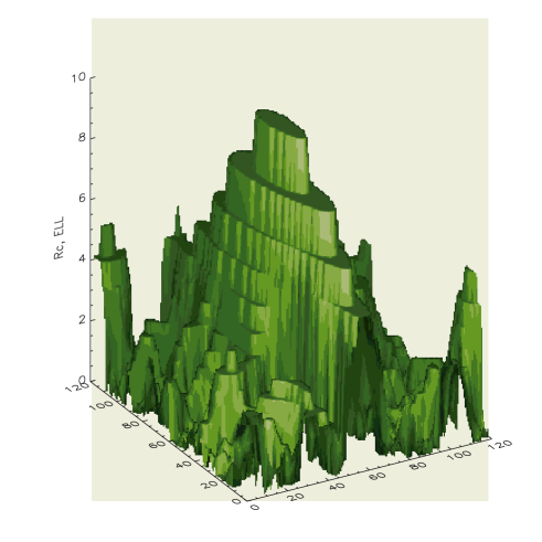
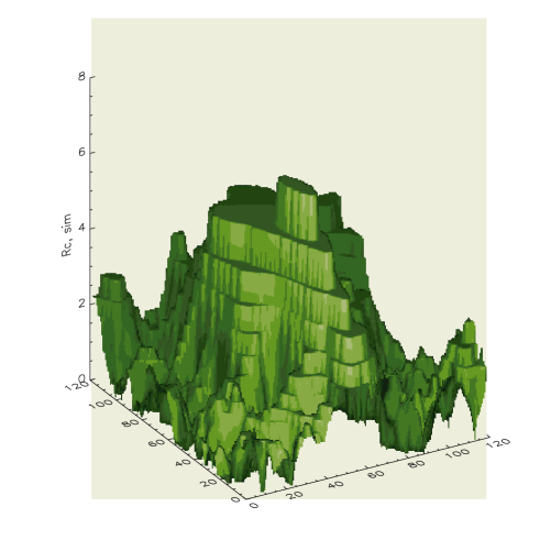
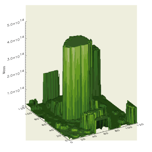
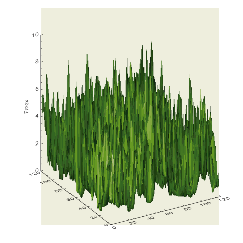
Figure 1: Upper panels: collapse radius fields $R_{c}$ for a section of the Lagrangian space of the $\Lambda$CDM simulation at redshift $z=0$. In the left panel we show the ELL prediction, and in the right panel the results from the simulation. Lower left panel: mass field for the same section; the mass field gives for each particle the mass of the halo it belongs to at $z=0$. Ungrouped particles are assigned 0 mass. Lower right panel: inverse collapse time $F_{\rm max}$ for the same section.

The $R_{c}$ field computed using LPT and obtained from the simulations at redshift $z=0$ are compared in figure 1. The two fields are remarkably similar, exhibiting the same structure of broad peaks, with the difference that the peaks of the simulation are lower, as anticipated by Monaco (1999). In figure 2 we show a more quantitative point-by-point comparison between the two fields. For display purposes, some random noise has been added to the discrete values of $R_{c}$; in this way the values lie in squares instead of points. There is a reasonably tight correlation between the predicted and numerical collapse-radius fields, which confirms the power of LPT to predict the mildly non-linear evolution of perturbations; it is noteworthy that this comparison does not involve free parameters. The correlation is quantified by the well-known Spearman rank correlation coefficient $r_{S}$ and Pearson’s linear correlation coefficient $r_{P}$, both reported in the panels of figure 1. (A high value of $r_{S}$ indicates the existence of a relation with moderate scatter, a high value of $r_{P}$ indicates the existence of a good linear relation.) The coefficients take rather high values of $\sim 0.8$, confirming in an objective and quantitative way the correlation.

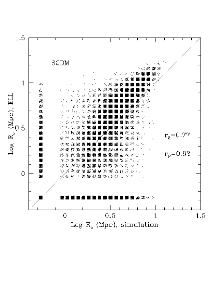
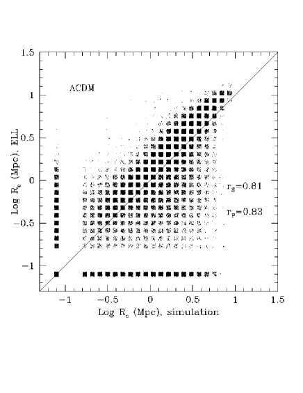
Figure 2: Comparison of the collapse radius fields $R_{c}$, as predicted by ELL, with the values found in the simulations, for a random sample of $\sim$20000 points for the SCDM model (left panel), and the $\Lambda$CDM model (right panel). For clarity some random noise has been added to the discrete $R_{c}$ values, so that they lie on squares instead of points.

However, as noted also in figure 1, the relation between the two $R_{c}$ fields is not unbiased: the simulated $R_{c}$ field is lower than the ELL one, especially at large $R$-values. The cause of this behaviour can be understood as follows. LPT predicts that after OC particles do not remain bound to the caustic region but move away from it, in contrast to what happens in the simulations. Therefore, as in this analysis particles are not explicitly restricted to the pre-OC (single stream) regime, the displacements in the simulation are always smaller than those predicted by LPT. As a consequence, the collapse radius obtained by the smoothed displacements of the simulation is lower than that predicted by LPT. This bias disappears at small radii, which are however dominated by numerical noise.

The difference between the LPT and simulation fields $R_{c}$ can also be quantified by the cumulative distribution of the $R_{c}$ fields as a function of $R$, or equivalently of the variance $\sigma^{2}(R)$. We will denote this function by $\Omega(<\sigma^{2})$, since it is also the fraction of mass collapsed on a scale $\geq R$ where the rms is smaller than $\sigma$. This quantity is used in the PS approach to obtain the mass function

$$Mn(M)dM=\bar{\rho}\frac{d\Omega}{d\sigma^{2}}\left|\frac{d\sigma^{2}}{dM}\right|dM.$$ (10)

The functions $\Omega(<\sigma^{2})$ from ELL and the simulations are compared in figure 3. The LPT curves are by construction independent of time and cosmology, so that only the $z=0$ LPT prediction in shown. In contrast, the $\Omega$ curves obtained from the simulations change with time. At late times, particles have crossed the structure they belong to many times and the numerical displacements differ more and more from the LPT ones. This is confirmed by the fact that the point of intersection between the $\Omega(<\sigma^{2})$ obtained from LPT and simulation roughly scales as $b(t)^{2}$. Most notably, the difference between predictions and simulations tends to vanish for the highest redshifts; in this case the particles have not had time to cross the structures, and their trajectories are very similar to the LPT ones. In all cases we notice that the numerical $\Omega(<\sigma^{2})$ functions become larger than the LPT ones at the smallest, unsmoothed scales, especially in the SCDM case and at higher redshift. This is most likely due to numerical noise present in the simulation, that enhances the level of non-linearity of the displacements, and in the SCDM case to the resampling from 360³ to 256³ grids.

Figure 3: Cumulative distributions $\Omega(<\sigma^{2})$ of the $R_{c}$ fields for the SCDM and $\Lambda$CDM simulations.

For comparison, we show in figure 3 also $\Omega(<\sigma^{2})$ from linear theory with $\delta_{c}=1.686$, which falls short of both the ELL prediction and the simulations. We have verified that linear theory (with Gaussian smoothing!) misses the collapse of many mass points that belong to filaments or to low mass halos. Decreasing $\delta_{c}$ to 1.5 improves the agreement only at the largest masses, but does not solve the problem at small masses. The Zel’dovich approximation severely under predicts $\Omega(<\sigma^{2})$ at large masses, but approaches the ELL curve for lower mass (Monaco 1997a). Consequently, using either linear theory or the Zel’dovich approximation instead of ellipsoidal collapse, would significantly decrease the accuracy of PINOCCHIO

We have also computed the $R_{c}$ field using full 3rd-order LPT. With respect to ELL, the fraction of collapsed points increases at small scales $R$, but decrease at large radii, because of the already mentioned inability of 3rd-order LPT to reproduce the spherical limit correctly (Monaco 1997a). We have verified that the correlation with the numerical $R_{c}$ field is noisier, and that the additional small-scale contribution of collapsed matter consists mainly of particles in filaments. Moreover, the computation is much more demanding than the ELL case. We conclude that there is no advantage in using the full 3rd-order LPT solution.

2.3 $R_{c}$ and the simulated halos

Having demonstrated the ability of LPT in predicting collapse in the OC sense (without free parameters), we need to decide whether OC may be of any use to predict which mass elements are going to end up in relaxed halos. In order to do so, we compute the ‘mass field’  from the simulation, which assigns to each grid vertex in the initial conditions, the mass of the halo that the corresponding particle ends-up in. Halos have been identified in the simulation using a standard friends-of-friends (FOF) algorithm, with a linking length 0.2 times the mean inter particle distance. The mass field is shown in figure 1c for the same slice of the $\Lambda$CDM simulation as the other panels. A FOF halo looks like a plateau, with the plateau’s height giving the halo’s mass. There is a broad agreement between the peaks in the $R_{c}$ and mass fields, because massive (low mass) objects are generally associated with large (small) smoothing radii. Consequently, there certainly is some connection between orbit crossed regions and relaxed halos. However, there are some important differences as well.

Not all the FOF points fall within the boundaries of the $R_{c}$ contours. This fact was already addressed by Monaco & Murante (1999), and is expected because the OC criterion tends to miss those infalling particles that have not made their first crossing of the structure. In fact, strictly speaking those should not be counted as belonging to the relaxed halo anyway. For SCDM, the fraction of FOF particles not predicted to be OC-collapsed ranges from $\sim$10 per cent at large masses to $\sim$20 per cent at smaller masses; smaller values are obtained for $\Lambda$CDM, where the fraction of collapsed mass is higher. This has a modest impact on the results, and is hardly noticeable in figure 1.

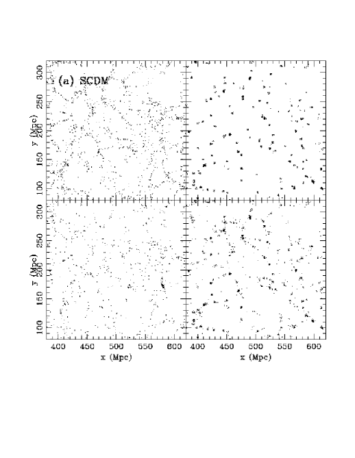
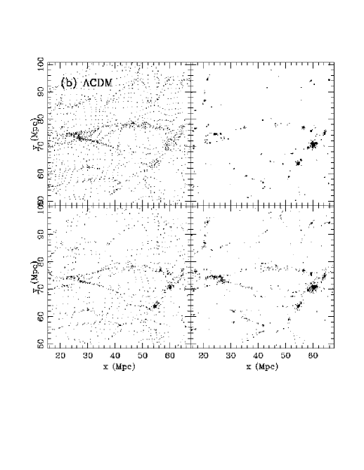
Figure 4: Final positions of particles at $z=0$ from a slice of the initial conditions for the SCDM model (plot a) and the $\Lambda$CDM model (plot b). In each plot, the left panels show those particles that are in filaments (i.e. that have undergone OC but are not assigned to a halo), the right panels show particles that are assigned to halos. Upper panels are obtained from the simulations, lower panels refer to PINOCCHIO.The large visual difference between the two cosmologies is mostly due to the very different box size used.

More importantly, the reverse is true as well: many particles assigned non-vanishing or even high $R_{c}$ values do not belong to a halo. These particles are in the moderately over dense filaments and sheets that connect the relaxed halos. These structures, although indeed in the multi-stream regime, are in a relaxation state very different from that of the halos. It is apparent that the removal of such sheets and filaments (hereafter referred to as filaments) is an important issue that needs to be addressed.

2.4 Computing the collapse time

Another feature apparent when comparing the mass and $R_{c}$ fields (figure 1) is that many FOF halos may correspond to a single broad peak of $R_{c}$. This makes the time-dependent $R_{c}$ field unsuitable for addressing the fragmentation of matter into halos and filaments. It is more convenient to follow a procedure similar to the merging cell model (Rodrigues & Thomas 1996; Lanzoni et al. 2000), i.e. recording for each mass point the largest $F$-value it reaches, or, in other words, the highest redshift at which the point is predicted to collapses in the OC sense (for SCDM it is simply $F=(1+z_{c})$, where $z_{c}$ is the collapse redshift). This is another way to solve the so-called cloud-in-cloud problem (Bond et al. 1991): a point that collapses at some redshift is assumed to be collapsed at all lower redshifts. We therefore record the following quantity:

$$F_{\rm max}({\bf q})\equiv\max_{R}[F({\bf q};R)].$$ (11)

Together with $F_{\rm max}$  we also store for each point the smoothing radius $R_{\rm max}$ at which $F=F_{\rm max}$, and the corresponding Zel’dovich velocity ${\bf v}_{\rm max}$ computed at the time $b(t)=1/F_{\rm max}$ appropriate for the smoothing radius $R_{\rm max}$.

In contrast to $R_{c}$, the inverse collapse time $F_{\rm max}$ evidently does not depend on time, while it does depend on the smoothing radius. The excursion set of those points where $F_{\rm max}$ is greater than some level $F_{c}$ gives the mass that has collapsed before the time $t_{c}$ that corresponds to $F_{c}$, at the highest resolution on the grid (i.e. without smoothing, $R=0$). The lower right panel of figure 1 plots the $F_{\rm max}$ field for the same section as the other panels. Within each large object identified in the mass field, $F_{c}$ has many small peaks that correspond to objects forming at higher redshifts. These peaks are modulated by modes on a larger scale that follow the excursions of the $R_{c}$ field. Those large scale modulations are ultimately responsible for the later merging of these small peaks into the massive object identified at late times. In this way, PINOCCHIO combines the information on the progenitors to reconstruct the merger history of objects, as described in detail in the next section.

3 Identification and merger history of halos

In the PS and excursion set approaches the mass of the objects that form at a scale R is simply estimated as

$$M\simeq\frac{4\pi}{3}\bar{\rho}R^{3}.$$ (12)

A more detailed treatment of the complex processes that determine the shape of the Lagrangian region to collapse into a single halo is required to get an improved description of the formation of the objects, and thus an improved agreement with simulations at the object-by-object level. In PINOCCHIO, this is done by generating realisations of the density field on a regular grid, computing the $F_{\rm max}$ field as explained above, and then ‘fragmenting’  the collapsed medium into halos and filaments by considering the fate of each particle separately. To enable a detailed comparison with the simulation, we will perform these steps on the initial conditions of the runs. Therefore, we can compare the properties of individual halos between the simulations and PINOCCHIO, not just the statistics of halos. Of course. PINOCCHIO can be applied to any realisation of a density field, including non-cubic grids and non-Gaussian perturbation fields. The fragmentation algorithm can even be applied to non-regular and non-periodic grids, if the FFT-based calculation of $F_{\rm max}$ is suitably modified.

Figure 5: Mass functions for the $\Lambda$CDM model at different redshifts indicated in the panel. Error bars denote Poissonian errors for the simulated mass function, continuous lines are the PINOCCHIO predictions, dotted and dashed lines are the PS and ST predictions, respectively.

The fragmentation code mimics the two main processes of hierarchical clustering, that is the accretion of mass onto halos and the merging of halos. The particles of the realisation are considered in order of descending $F_{\rm max}$-value, i.e. in chronological order of collapse. At a given time the particles that have already collapsed will be either assigned to a specific halo, or associated with filaments. Because of the continuity of the transformation between Lagrangian and Eulerian coordinates, equation 1, a particle must touch a halo in the Lagrangian space if it is to accrete on it. Thus a collapsing particle can accrete only onto those halos that are ‘touched’ by it, i.e. that already contain one of its 6 nearest neighbours in the Lagrangian space of initial conditions (we call these particles Lagrangian neighbours). To decide whether the particle does accrete onto a touching halo, we displace it to the Eulerian space according to its ${\bf v}_{\rm max}$ velocity. The halo is displaced to its Eulerian position at the time of accretion, using the average velocity of all its constituent particles. In the following we express sizes and distances in terms of the grid spacing. The size $R_{\rm N}$ of a halo of $N$ particles is taken to be

$$R_{\rm N}=N^{1/3}.$$ (13)

The collapsing particle is assumed to accrete onto the halo, if the Eulerian (comoving) distance $d$ between particle and halo is smaller than a fraction of the halo’s size $R_{\rm N}$

$$d<f_{\rm a}\times R_{\rm N}.$$ (14)

The free parameter $f_{\rm a}$, which is smaller than one, controls the over density that the halo reaches in the Eulerian space, $1+\delta_{\rm halo}\sim 3/4\pi f_{\rm a}^{3}$. Therefore, this criterion selects halos at a given over density, making it similar to the usual FOF or similar selection criteria. The value of the $f_{\rm a}$ parameter is fixed in Appendix A to $\sim 0.25$. Then, the halos reach a much lower over density than the value $\sim 200$ used in simulations; Zel’dovich velocities (and LPT velocities in general) are not accurate enough to reproduce such high densities for the relaxed halos. However, PINOCCHIO only attempts to identify the halos, not compute their internal density profile as well.

Figure 6: Eulerian correlation function (upper panels) and Lagrangian correlation function (lower panels) for the $\Lambda$CDM models at three redshifts indicated in the panel, and for two mass ranges. Symbols refer to simulation results, lines to PINOCCHIO predictions. Filled squares and continuous lines: correlation function for low mass halos (mass $M$ from $6.3\times 10^{11}$ to $3\times 10^{12}\ M_{\odot}$), open squares and dashed lines: correlation function for massive halos ($M>3\times 10^{12}\ M_{\odot}$).

When a collapsing particle touches two (or more) halos in the Lagrangian space, then we use the following criterion to decide whether the two halos should merge. We compute the Eulerian distance $d$ between the two halos at the suspected merger time using the halo velocities described above. The halos are deemed to merge when $d$ is smaller than a fraction of the Lagrangian radius of the larger halo:

$$d<f_{\rm m}\times\max(R_{\rm N1},R_{\rm N2}).$$ (15)

This condition amounts to requiring that the centre of mass of the smaller halo, say halo 2, is within a distance $f_{\rm m}R_{\rm N1}$ of the centre of mass of the larger halo 1. The value of the $f_{\rm m}$ parameter is fixed in Appendix A to 0.35.

We note that PINOCCHIO is not restricted to binary mergers. In principle, a particle has 6 Lagrangian neighbours so up to 6 halos may merge at the same time. In practice binary mergers are the most frequent, but ternary mergers also occur, while mergers of four halos or more are rare.

In more detail, the fragmentation code works as follows. We keep track of halo (or filament) assignment for all particles. For each collapsing particle we consider the halo assignment of all Lagrangian neighbours; touching halos are those to which a Lagrangian neighbour has been assigned. The following cases are considered:

(i) If none of the neighbours have collapsed, then the particle is a local maximum of $F_{\rm max}$. This particle is a seed for a new halo of unit mass, created at the particle’s position.

(ii) If the particle touches only one halo, then the accretion condition is checked. If it is satisfied, then the particle is added to the halo, otherwise it is marked as belonging to a filament. The particles that only touch filaments are marked as filaments as well.

(iii) If the particle touches more than one halo, then the merging condition is checked for all the touching halo pairs, and the pairs that satisfy the conditions are merged together. The accretion condition for the particle is checked for all the touching halos both before and after merging (when necessary). If the particle can accrete to both halos, but the halos do not merge, then we assign it to that halo for which $d/R_{\rm N}$ is the smaller. Occasionally, particles fail to accrete even though the halos merge.

(iv) When a particle is accreted onto a halo, all filament particles that neighbour it are accreted as well. This is done in order to mimic the accretion of filaments onto the halos. Notice that up to 5 filament particles can flow into a halo at each accretion event.

This fragmentation code runs extremely quickly, in a time almost linearly proportional to the number of particles. At late times, slightly more time is spent in updating the halo assignment lists in case of mergers, but this does not slow down the code much.

In high density regions where most of the matter has collapsed, it can happen that pairs of halos that are able to merge are not touched by newly collapsing particles for a long time. This problem can be solved by keeping track of all the pairs of touching halos that have not merged yet, and checking the merging condition explicitly at some time intervals. Such a check slows the code down significantly, and has only a moderate impact on the results when the fraction of collapsed mass at the grid scale is large. Similarly, the accretion of filament particles on to halos can be checked at some given time intervals, but again, the impact is modest on the results but the increase in computer time may be substantial

Figure 7: Count-in-cell analysis of the halo catalogues at $z=0$. Left and right panels show results for the mass ranges indicated. Symbols refer to simulation results, lines to PINOCCHIO predictions. Continuous, dotted and dashed lines (or squares, stars and circles) refer to cell sizes of 2, 5 and 10 Mpc (1.3, 3.25 and 6.5 Mpc/h).

While the dynamical estimate of collapse time does not introduce any free parameter, the fragmentation process does. The same happens in the simulation, where any halo-finding algorithm has at least one free parameter, such as the linking length for FOF halos. This is because the definition of what constitutes a DM halo is somewhat arbitrary, and hence also the corresponding mass function is not unique (Monaco 1999). Fortunately, different clump-finding algorithms usually give similar results, so that this ambiguity is in general not a real problem. In the following, the best fit parameters for PINOCCHIO will be chosen so as to reproduce the mass function of the FOF halos of the simulations, with linking length equal to 0.2 times the inter-particle distance, at many redshifts. We have checked with one SCDM output that the differences in the halos as defined by the HOP (Eisenstein & Hut 1998) and SO (Lacey & Cole 1994) algorithms are much smaller than the accuracy with which we are able to recover the FOF halos.

The five free parameters of the fragmentation code, and the determination of their best-fit values, are described in Appendix A. Note that the results shown paper I use a more limited set of three free parameters, which is adequate to describe large-volume realisations such as that of the SCDM simulation, while the larger set of parameters described in Appendix A has a more general validity.

The ability of PINOCCHIO to distinguish OC particles that collapse into halos versus those that remain in filaments, is shown in figure 4. In this figure we plot the final position of the particles, as given by the simulation output at redshift $z=0$, for a section of the initial conditions of the SCDM and $\Lambda$CDM simulations. Left panels show only the filament particles, defined as those which are in OC according to $R_{c}$ but do not belong to any halo. Right panels show only those particles that are in halos. Upper panels show the result from the simulation, lower panels the PINOCCHIO predictions. Clearly, PINOCCHIO is able to distinguish accurately halos from filaments, even though some filament particles are interpreted as halo particles and vice versa. When compared with figures 6 and 7 of Bond et al. (1991), figure 4 shows the marked improvement of PINOCCHIO with respect to the extended PS approach. We want to stress that filaments are important in their own right. For example, most of the Lyman-$\alpha$ absorption lines seen in the spectra of distant quasars are produced in filaments (e.g. Theuns et al. 1998), so it will be useful to be able to generate catalogues of halos and filaments.

4 Detailed comparison to simulations.

4.1 Statistical comparison

The comparisons of PINOCCHIO and FOF mass and correlation functions for the SCDM simulation were presented in paper I, using the more limited set of three free parameters. The results with the full five-parameter set are very similar and are not shown here. In figure 5, we compare the mass function computed using PINOCCHIO and the $\Lambda$CDM $N$-body simulation. The FOF halos were identified as explained above. For reference, we also plotted the PS and Sheth & Tormen (1999, hereafter ST) mass functions. The choice of parameters reported in Appendix A produces a PINOCCHIO mass function which falls to within $\sim$5 per cent of the simulated one from $z=5$ to $z=0$, for all mass bins with more than 30-50 particles per halo and for which the Poisson error bars are small. The only residual systematic is a modest, $\sim$10-20 per cent underestimate at the highest-mass bins and highest redshift. An accuracy of better than 10 per cent on the mass function for a given realisation is perfectly adequate for most applications, as it is usually smaller than the typical sample variance as well as the intrinsic accuracy of $\sim 20-30$ per cent with which the mass function of N-body simulations is defined. Because PINOCCHIO is calculated for the same initial conditions as the simulation, Poisson error bars are not the correct errors to use for this comparison (notice that the Poisson error bars of the PINOCCHIO mass function are obviously very similar to those of the numerical one). We show them both for comparison with PS and ST and to understand which mass bins are affected by small number statistics.

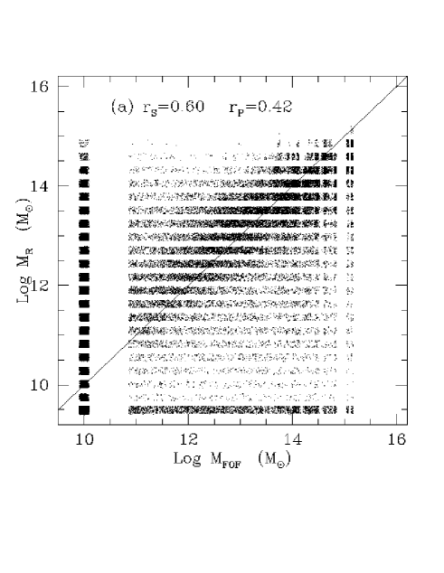
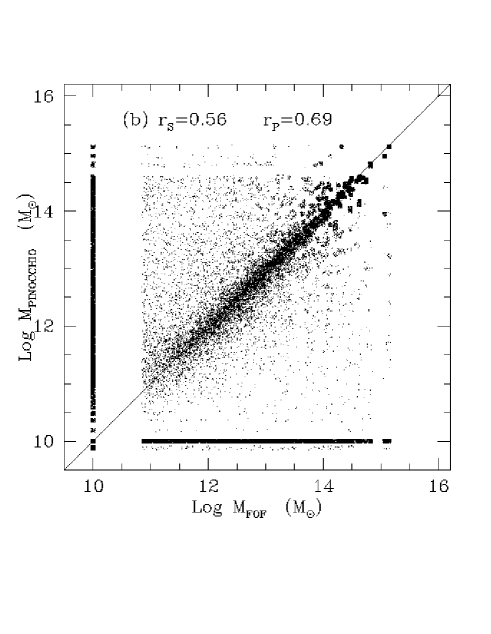
Figure 8: Comparison of the mass fields for FOF halos identified in the $\Lambda$CDM simulation with that obtained from the $R_{c}$ field using the PS mass-radius relation (equation 12, left panel) and using PINOCCHIO (right panel). For clarity some random noise has been added to the mass field values, especially to that obtained from the discrete $R_{c}$ field.

Taking the ST mass function (or the analytic fit of Jenkins et al. 2001) as a bona fide estimate, we have checked the validity of PINOCCHIO in reproducing the mass function of halos in a wide variety of cosmologies and box sizes (see Appendix A). The fit of the mass function is found to be still good even for halo masses as small as $10^{5}$ M_⊙ ($\Lambda$CDM cosmology), at a redshift high enough to avoid that the whole box goes non-linear.

Strictly speaking the agreement between the mass functions of PINOCCHIO and the simulated ones is not a proper comparison of prediction with numerical experiment, as the fit is achieved by tuning the free parameters discussed in Section 3. However, the very existence of a limited set of parameters that allows to achieve such a good agreement in different cases (SCDM and $\Lambda$CDM, PKDGRAV and Hydra, small and large boxes) is a very important result. As shown also in figure 5, PINOCCHIO improves the fit with respect to PS, giving an accuracy very similar to the ST fit. Jenkins et al. (2001) showed that the ST fit underestimates the knee of the FOF mass function by $\sim$10-20 per cent; we have verified that when this difference is evident the best fit PINOCCHIO mass function is more similar to the numerical one and to the Jenkins et al. (2001) fit than to the ST mass function. This is evident in figure 1 of paper I (where the residuals of the $z=0$ mass functions are shown), but is hardly noticeable in figure 5, where Poisson errorbars are larger. The comparison with the $\Lambda$CDM simulation shows that the fit is very good also down to the low mass tail $M\sim 10^{11}\ M_{\odot}$ or $M/M_{*}\sim 10^{-2}$ ($M_{*}$ denotes the characteristic mass of the PS mass function, such that $\sigma^{2}(M_{*})=\delta_{c}^{2}$; see, e.g., Monaco 1998).

In the PS and excursion set approaches, the mass function is ‘universal’ when expressed in terms of the variable $\Omega(<\sigma^{2})$ already defined in Section 2.2 (equation 10), which in this case gives the fraction of mass collapsed into objects larger than $M(\sigma^{2})$ (with the mass given by equation 12). The mass functions obtained from a large set of numerical simulations is indeed found to be universal to within $\sim$30 per cent (Jenkins et al. 2001). The PINOCCHIO mass function is not by construction universal, yet we find it to be nearly universal once the resolution effects described in Appendix A are taken into account.

However, the mass function of the Governato et al. (1999) SCDM simulation used here shows an excess of massive halos at high redshift. This was already noticed by Governato et al., and quantified as a drift of the $\delta_{c}$ parameter from $\sim$1.5 at high redshift to $\sim$1.6 at $z=0$. This trend is not confirmed by other simulations (Jenkins et al. 2001), nor by our $\Lambda$CDM simulation presented here. We find that PINOCCHIO reproduces the weak trend of Governato et al. (1999) in the SCDM simulation, but also the lack of such a trend in the $\Lambda$CDM one. We conclude therefore that this effect is likely to be linked to the initial conditions generator, which is different for the two realisations (see Appendix A for more details). Recall that the PINOCCHIO mass functions refer to the same initial conditions as were use to perform the simulations.

In figure 6 we show the correlation function of halos as a function of mass, both in Eulerian and in Lagrangian space. The correlation function has been computed using a standard pair counting algorithm. The agreement between PINOCCHIO and the simulation is very good down to scales of a few grid cells, i.e. $\sim$1-2 comoving Mpc/h (larger for rarer objects), below which the PINOCCHIO correlation functions become negative. This is in agreement with what found in paper I for the SCDM simulation. The differences are of order $\sim$10-20 per cent in amplitude and $\la$10 per cent in terms of scale at which a fixed amplitude is reached. This means that both the correlation length $r_{0}$, at which $\xi(r_{0})=1$, and the length at which $\xi=0$ are reproduced with an accuracy of better than 10 per cent. This is an improvement with respect to the ST formalism, where the accuracy is of order $\sim$20 per cent (Colberg et al. 2001). More importantly, the trends of increased correlation for the more massive halos, or for halos of a given mass with increasing redshift, are both well reproduced. The correlation functions in the Lagrangian space are noisier, and are reproduced with somewhat larger error, especially at $z=0$ where they are slightly overestimated; however this error does not seem to propagate to the Eulerian correlation functions.

The two-point correlation function gives only a low-order statistics of the spatial distribution of a set of objects. To probe the accuracy of the PINOCCHIO results at higher orders, we have performed a count-in-cell analysis of the halo distribution, which, at variance with the correlation function, depends also on the phases of the space distribution of the halos. This is shown in figure 7 for galactic-sized ($10^{12}M_{\odot}\leq M\leq 10^{13}M_{\odot}$) and group-sized ($M\geq 10^{13}M_{\odot}$) halos of the $\Lambda$CDM realisation, and cell sizes of 2, 5 and 10 Mpc (corresponding to 1.3, 3.25 and 6.5 Mpc/h). The count-in-cells curves are well reproduced by PINOCCHIO, although their skewness is slightly underestimated, especially for larger cells and smaller masses. In particular, the void probability $P_{0}$ of finding no halos in the cell is reproduced with an accuracy no worse that a few percent when it takes values in excess of 0.6.

4.2 Point-by-point and object-by-object comparison

The PINOCCHIO approach is not just limited to making accurate predictions for statistical quantities such as the mass and correlation functions, but is also able to predict halo properties that correspond in detail to those obtained from simulations. This is in contrast to the PS approach, where the object-by-object agreement is very poor (White 1996, but see Sheth et al. 2001 for a different view).

Figure 9: Comparison on an object-by-object level of halos identified by PINOCCHIO and found in the $\Lambda$CDM simulation, using a variety of statistics. Continuous, dotted, short-dashed and long-dashed lines refer respectively to redshifts $z=0$, 1, 2 and 4. Top panel: fraction $f_{\rm cl}$ of cleanly assigned objects; middle panel: fraction $f_{\rm split}$ of non-cleanly assigned objects; bottom panel: average overlap $f_{\rm ov}$ for cleanly assigned objects. The vertical lines in the top panel indicate halos with 10, 100, 10³, 10⁴ and 10⁵ particles (heavy lines) or 50, 500, 5$\times$10³ and 5$\times$10⁴ particles (light lines).

Agreement at the ‘point-by-point level’  requires that each particle is predicted to reside in the correct halo with the correct mass. Whether this agreement holds can be checked by comparing the mass fields already defined in section 2.2 (an example of which is shown in figure 1c). We note that this type of analysis is similar to that of Section 2.2, where the point-by-point agreement was checked for the $R_{c}$ fields. In the PS approach, the mass of the halo to which a particle belongs is estimated as in equation 12, with the $4\pi/3$ valid for top-hat smoothing (or sometimes left as a free parameter). In this case the mass field is simply related to the $R_{c}$ field. A comparison between the mass fields obtained from the same $R_{c}$ field of figure 2 (with arbitrary normalisation) and that of the simulation, $M_{\rm FOF}$, reveals only a poor correlation, as shown shown in figure 8 (left panel) for a random sample of $\sim$20000 particles extracted from the $\Lambda$CDM simulation. The tightness of the correlation is again quantified by the $r_{S}$ and $r_{P}$ coefficients. This figure is similar to figure 8 of White (1996) and figure 2 of Sheth et al. (2001), with the difference that here the $R_{c}$ curve were computed with ELL instead of with linear theory (and Gaussian smoothing instead of top-hat). The point-by-point agreement is much better with PINOCCHIO (right hand panel), where the linear correlation coefficients $r_{P}$ jumps from 0.42 to 0.69, demonstrating the increase in accuracy. Clearly, the improvement of PINOCCHIO in the point-by-point comparison is not primarily due to the more accurate dynamical description of collapse. Rather it is due to the much more accurate description of the shape of the collapsing region, which is not restricted to the simple PS relation of equation 12.

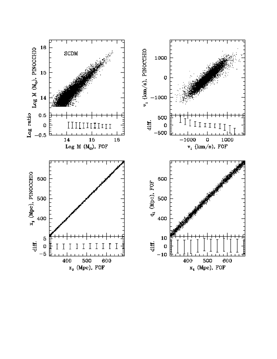
Figure 10: Difference in mass, position and velocity, $\log M$, $x_{1}$ and $v_{1}$ respectively, as estimated by PINOCCHIO and found from the simulation, for cleanly assigned halos. The scatter around the mean is plotted below each panel. The lower right panels show for comparison the displacement of halos according to the simulation. The first set of panels refer to the SCDM simulation, the second to the $\Lambda$CDM one

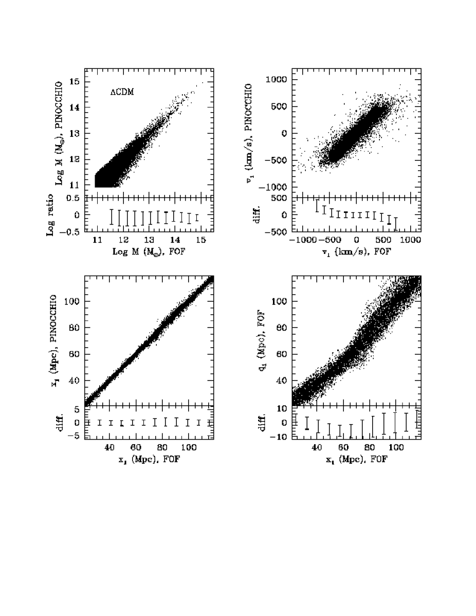
Figure 10: (continued)

While the linear correlation coefficients improves significantly going from $R_{c}$ to the PINOCCHIO mass field, the Spearman correlation coefficient $r_{S}$ does not change much, since both panels contain a large number of outliers. These are particles that lie at the border of halos, and are assigned to a halo by the simulation but not by PINOCCHIO, or vice versa. Such outliers are expected whenever the boundaries of halos in the Lagrangian space are not perfectly recovered. On the other hand the presence of such outliers is not very important when the catalogue of objects is considered.

We next investigate the agreement of PINOCCHIO with the simulations at the object-by-object level, a coarser level of agreement but more relevant in practice. The degree of matching between halo catalogues is quantified as in paper I. For each object of one catalogue, the objects of the other catalogue that overlap for at least 30 per cent of the Lagrangian volume are considered. Two halos from different catalogues are ‘cleanly assigned’  to each other, when each overlaps the other more than any other halo. The fraction of halos not cleanly assigned is $f_{\rm split}$. The remainder 1–$f_{\rm cl}$–$f_{\rm split}$ is the fraction of objects of one catalogue that does not overlap with any halo in the other catalogue. These fractions quantify the level to which two catalogues describe the same set of halos. Another useful quantity is $f_{\rm ov}$, the average fraction that halos overlap when they are cleanly assigned. All these estimators depend on whether PINOCCHIO is compared with simulations or vice-versa, but in general that difference is small as long as the comparison is good.

In figure 9 we show the values of these three indicators of the agreement between the two halo catalogues as a function of halo mass, for $\Lambda$CDM model; the SCDM case was shown in paper I. The agreement is very good at higher redshift with $\sim$80-90 per cent of objects cleanly assigned when the halos have at least 50 particles. The degree of splitting is only $\la$5 per cent, while the average overlap of cleanly-assigned objects $f_{\rm ov}$ ranges from 60 per cent to 70 per cent nearly independent of mass and encouragingly larger than the 30 per cent lower limit. These results are in agreement with the SCDM ones presented in paper I. The agreement is slightly worse at lower redshift, with $f_{\rm cl}$$\ga$70 per cent for halos with at least 100 particles, and a $f_{\rm split}$$\sim$5–10 per cent. Within perturbative approaches there is obviously no advantage in going to higher resolution, as the accuracy of LPT worsens with the degree of non-linearity (see figure 15) and with it all the results. Anyway, the agreement is still very significant for the last output, with a high fraction of cleanly assigned objects and a modest degree of splitting. In any case the results always improve with increasing number of particles. Monaco (1997a) estimated that LPT would break down when $\sim$50 per cent of the mass has undergone OC. Therefore, the agreement shown in figure 9 (and also in figure 4) is better than expected.

Figure 11: The effects of numerical resolution for simulations and for PINOCCHIO. Halo masses for a random set of particles from the $256^{3}$ $\Lambda$CDM realisation as determined from the simulation and by PINOCCHIO (left and right panels respectively) are compared with the masses from the $\Lambda$CDM128 simulation.

In figure 10 we show the accuracy with which PINOCCHIO is able to estimate mass, Eulerian position and velocity of the cleanly assigned objects. In particular, we show both for SCDM and $\Lambda$CDM the scatter plots of the masses, and of velocity and position along one coordinate axis. For comparison, the scatter plot of the displacements of FOF halos from the initial to the final positions are shown as well. Masses are recovered with an accuracy of $\sim$30 per cent for SCDM and $\sim$40 per cent for $\Lambda$CDM, nearly independent of mass. The average value is slightly biased, which results from our constraint in reproducing the mass function. Positions are recovered with a 1D accuracy of $\sim$1 Mpc, slightly depending on the box size and much smaller than the typical displacements, while velocities are recovered with a 1D accuracy of $\sim$150 or 100 km/s for SCDM or $\Lambda$CDM. In general, the velocities of the fastest moving halos are underestimated. This could be fixed by extending the calculation of velocities to third order LPT, although a straightforward extension has been found not to work.

The comprehensive analysis of the statistical properties of the PINOCCHIO halos and their merger histories, presented here and in Taffoni et al. (2001), demonstrate that the statistical properties of halos are always well reproduced for $N>30-50$ particles, so that the degrading of quality of the object-by-object comparison with time (non-linearity) is due to random noise, which does not induce significant systematics and thus does not hamper the validity of the halo catalogues.

We stress that these comparisons are pure predictions of PINOCCHIO, in the sense that the free parameters of the method are constrained by the $z=0$ mass function alone. The good agreement with the numerical simulations confirms that PINOCCHIO is a successful approximation to the gravitational collapse problem in a cosmological and hierarchical context.

4.3 Resolution effects

As discussed above, PINOCCHIO halos resemble the FOF ones closely if they possess a minimum number of particles of around 30-100. Statistical quantities are well reproduced for halos with at least 30-50 particles. These limits are comfortably similar to the minimum number of particles needed by a simulation to produce reliable halos. To show this we plot in figure 11, for a random set of particles, the mass fields (i.e. the mass of the halo the particle belongs to) as determined by the 128³ or 256³ $\Lambda$CDM runs, both for the simulations and for PINOCCHIO. The result is shown at $z=0$. There is considerable scatter between the masses of the halos determined from simulations with different resolutions. This scatter is less than between PINOCCHIO and simulations, but not by much. This result is similar at higher redshifts. More details are given in Appendix B, where it is shown that the match of the $\Lambda$CDM and $\Lambda$CDM128 halo catalogues shows a drop in the number of cleanly assignments for halos smaller than $\sim$30 particles (figure 16a), very similar to that shown in figure 9.

This results suggests that resolution affects PINOCCHIO in a similar way as it affects numerical simulations. Better resolution leads to increased scatter in the identification of halos, since the structures become more non-linear. For instance, we have verified that more massive halos are reconstructed slightly better by the 128³ PINOCCHIO run than by the 256³ one. This is because at higher resolution, PINOCCHIO may decide to break-up a more massive halo in two. The degrading of the quality is modest and amounts to increased random noise which does not bias significantly the statistics of the halos.

5 Angular momentum of the DM halos

Halos are thought to acquire their angular momentum from tidal torques exerted by the large-scale shear field while they are still in the mildly non-linear regime (Hoyle 1949; Peebles 1969; White 1984; Barnes & Efstathiou 1987; Heavens & Peacock 1988). In this hypothesis it is possible to estimate the angular momentum of halos using the Zel’dovich (1970) approximation or higher-order LPT (Catelan & Theuns 1996a,b). The biggest difficulty in this calculation is to identify the Lagrangian patch that is going to become a halo.

However, it was recently shown by Porciani, Hoffmann & Dekel (2001a,b) that the Zel’dovich approximation is unable to give very accurate predictions of the spin of halos, as the highly non-linear interactions of neighbouring halos tend to randomize their spins. Assuming to know exactly which particles are going to flow into a halo at $z=0$ and using the Zeld’ovich approximation to compute the large-scale shear field, Porciani et al. (2001a) were able to recover the final angular momentum of the DM halos with an average alignment angle (defined as the angle between true and reconstructed spins) of no better than $\sim$40^∘.

Their analysis highlights the difficulty in predicting a higher-order quantity such as the spin of DM halos. The same calculation of spin with N-body simulations is subject to debate. Comparing our $\Lambda$CDM and $\Lambda$CDM128 simulations, we show in Appendix B that for an order-of-magnitude estimation of angular momentum at least 100 particles per groups are required, while a more robust estimation requires at least ten times more particles. This is at variance with other quantities, such as halo mass and velocity, that converge more rapidly. In the following we will restrict our analysis to groups larger than 100 particles.

With respect to the analysis of Porciani et al (2001a), the PINOCCHIO code presents the advantage of predicting with good accuracy the instant at which particles get into the halo, while the actual shape of the halo in the Lagrangian space is recovered with some noise, especially in the external borders that in fact contribute most to the angular momentum. We have verified that the direction of the largest axis of the inertia tensor of the halos in the Lagrangian space is recovered within an alignment angle of $\sim$20^∘, while ellipticity and prolateness are correctly reproduced, although with much scatter.

The estimate of the angular momentum of halos is easily performed within the fragmentation code, with negligible impact on its speed. When two halos with angular momenta ${\bf L}_{1}$ and ${\bf L}_{2}$ merge, the spin ${\bf L}_{\rm merg}$ of the merger is estimated as:

$${\bf L}_{\rm merg}={\bf L}_{1}+{\bf L}_{2}+{\bf L}_{\rm orb},$$ (16)

where ${\bf L}_{\rm orb}$ is the orbital angular momentum of the two halos:

$${\bf L}_{\rm orb}=M_{1}(\Delta{\bf q}_{1}\times\Delta{\bf v}_{1})+M_{2}(\Delta{\bf q}_{2}\times\Delta{\bf v}_{2}).$$ (17)

Here $\Delta{\bf q}_{i}\equiv{\bf q}_{i}-{\bf q}_{\rm cm}$, $\Delta{\bf v}_{i}\equiv{\bf v}_{i}-{\bf v}_{\rm cm}$, with $i=1,2$, ${\bf q}_{\rm cm}$ and ${\bf v}_{\rm cm}$ the position and velocity of the centre of mass. It is worth noticing that the use of Lagrangian coordinates ${\bf q}$ is justified by the parallelism of displacements and velocities. Following Catelan & Theuns (1997a), we stop the linear growth of velocities not at the time of merger $t_{\rm merge}$ but at the time $t_{\rm grow}$ defined as:

$$t_{\rm grow}=0.5t_{\rm merge}$$ (18)

where $t$ is physical time. This is a suitable generalisation of the concept of ‘detaching’ of the perturbation from the Hubble flow. The case of accretion is treated as a merger with a 1-particle halo which carries zero spin.

The so-obtained angular momenta obey a mass–spin relation which is roughly consistent with that of the FOF groups. This is shown in the left panels of figure 12 for the $\Lambda$CDM simulation. Although qualitatively similar, the PINOCCHIO relation overestimates the FOF one by some factor which is larger for the smaller halos. If the lower value of the spin is due to the higher degree of non-linear shuffling suffered by halos because of tidal interaction with neighbours, this trend of having lower-mass halos more randomized than higher-mass ones is in agreement with that suggested by Porciani et al. (2001a).

It is useful to improve this prediction, so as to obtain angular momenta for the halos with accurate statistical properties. To this aim we decrease each component of the spin at random, following the simple rule:

$$L_{i}^{\rm new}=L_{i}\times((1-f_{\rm spin})+f_{\rm spin}\times f_{\rm rand}),$$ (19)

where $f_{\rm spin}=f_{0}+f_{1}(M/M_{*}(z))$ (forced to $0\leq f_{\rm spin}\leq 1$) and $f_{\rm rand}$ is a random number ($0<f_{\rm rand}<1$). The two parameters $f_{0}$ and $f_{1}$ are fixed so as to reproduce at best the mass–spin relation of figure 12. Optimal values are $f_{0}=0.8$ and $f_{1}=0.15$. The right panels of figure 12 show the resulting mass–spin relations, which agrees fairly well with the FOF ones.

Figure 12: Mass–spin relation for dark-matter halos. Contour lines trace the levels of 0.2, 1, 2 and 4 halos per decade in $\log M$ ($M_{\odot}$) and $\log L/M$ (km/s Mpc, physical units). Continuous and dotted lines show the contours for FOF and PINOCCHIO halos respectively. Dashed lines give the scaling $L\propto M^{5/3}$ (Catelan & Theuns 1996a). Upper panels: $z=0$; lower panels: $z=3$. Left panels: no correction; right panels: spin corrected as in equation 19.

Apart from the mass–spin correlation shown in figure 12, the angular momentum is known to be nearly independent of other halo properties (Ueda et al. 1994; Cole & Lacey 1996; Nagashima & Gouda 1998; Lemson & Kauffman 1999; Bullock et al. 2001; Gardner 2001; Antonuccio-Delogu et al. 2001), with the exception of a weak dependence with the merger history of the halos. The dependence of spin on the environment is still debated (Lemson & Kauffman 1999; Antonuccio-Delogu et al. 2001). Gardner (2001) has shown that halos that have suffered a major merger tend to have higher spin. In figure 13 we show that this trend is successfully reproduced by PINOCCHIO halos. Merged halos at $z=0$ have been selected by requiring that the second largest progenitor halo at $z=0.25$ is larger than 0.3 times the final halo mass. To extract the mass–spin relation, we define the quantity $\lambda\equiv LogL-1.5(LogM/M_{*})$. As apparent in figure 13, the $\lambda$-distribution of the merged halos is biased toward larger $\lambda$-values both for the simulation and for the PINOCCHIO halos, although the trend may be slightly underestimated by PINOCCHIO.

The agreement at the object-by-object level is in line with the intrinsic limits of perturbative theories found by Porciani et al. (2001a). Figure 14 shows the alignment angle $\theta$ for the spins of cleanly matched FOF and PINOCCHIO halos, and their average values computed in bins of mass (error flags indicate the rms around the mean). While the left panel shows all halos, the right panel is restricted to those pairs of halos that overlap by more than 70 per cent. The average angle is significantly smaller than 90^∘, highlighting a significant correlation of PINOCCHIO and FOF spins. However, the alignment is at best as high as $\sim$60^∘. This is mostly due to errors in the definition of the halo, as shown by the right panel, where the best reconstructed halos with more than 1000 particles show an average alignment angle of $\sim$30–40^∘, consistent with the intrinsic limit quoted by Porciani et al. (2001a).

To conclude, the prediction of angular momentum of halos is severely hampered by the intrinsic limits of linear theory described by Porciani et al. (2001a) and further worsened by the error made by PINOCCHIO in assigning particles to halos. The correct statistics is reproduced only by introducing two more ‘fudge’ free parameters, while the object-by-object agreement is poor although significant. However, even N-body simulations do not converge rapidly in estimating this quantity (see Appendix B). Moreover, the important spin–merger correlation is recovered naturally. Although we do not claim this result as a big success, we notice that PINOCCHIO is, to our knowledge, the only perturbative algorithm able to predict the spin of halos at the object-by-object level. Moreover, the prediction of spins comes at almost no additional computational cost, and the whole acquisition history of angular momentum can be followed for each halo. Thus, we regard the use of the angular momenta provided by PINOCCHIO as a viable alternative to drawing them at random from some distribution that fits N-body simulations (Cole et at. 2000; Vitvitsaka et al. 2001; Maller, Dekel & Somerville 2001).

Figure 13: Correlation between spin and merging history. Continuous lines: all halos; dashed lines: halos that have suffered a major merger. Left panels: PINOCCHIO predictions; right panels: simulation. Upper panels: halos with $M\geq 10^{12}\ M_{\odot}$; lower panels: halos with $M\geq 10^{13}\ M_{\odot}$.

6 Discussion

PINOCCHIO is an approximation to the full non-linear gravitational problem of hierarchical structure formation in a cosmological setting, in contrast to the mostly statistical approaches such as the PS prescription. The good agreement in detail between PINOCCHIO and FOF halos identified in simulations, explains the ability of the method to generate reliable halo catalogues. It also demonstrates that the underlying dynamical approximations work well. With respect to the results of Monaco (1995; 1997a,b), PINOCCHIO addresses successfully the geometrical problem of the fragmentation of the collapsed medium into objects and filaments.

While a direct analytical rendering of the fragmentation prescription as used in PINOCCHIO seems very complex, because it requires knowledge of spatial correlations to high order, analytical progress might nevertheless be possible. For instance, Monaco & Murante (1998) proposed to generalise the mass-radius relation of PS, to allow a more general distribution of masses to form at a given smoothing radius. This was formulated in terms of a ‘growing’  curve for the objects, that gives the fraction of mass acquired by the object at a given smoothing radius. The mass function is then obtained by a deconvolution of the $\Omega(<\sigma^{2})$ function (as obtained from ELL collapse, like in figure 3) with the growing curve of the objects. This growing curve could be estimated from the results of PINOCCHIO, giving an improved analytical expression for the mass function. But in the case of Gaussian smoothing merging histories cannot be computed from the excursion set formalism, because the trajectories are strongly correlated (Peacock & Heavens 1990; Bond et al. 1991), so that the random walk formalism cannot be used. Moreover, it is impossible from such an approach to have full information on the spatial distribution of objects. So, such analytic extensions of PINOCCHIO would not be as powerful as the full analysis. Besides, analytic formalisms based on peaks (Manrique & Salvador Sole 1995; Hanami 1999) are manageable only when linear theory is used. We therefore regard methods like PINOCCHIO which are based on an actual realisation of the linear density field, as a good compromise between performing a simulation, and getting only statistical information from a PS like approximation.

As mentioned in the introduction, similar methods have been proposed in the literature, such as the peak-patch method of Bond & Myers (1996a), the block model of Cole & Kaiser (1988), and the merging cell model of Rodrigues & Thomas (1996) and Lanzoni et al. (2000). A qualitative comparison with peak-patch reveals a similar accuracy in reproducing the masses of the objects. From figure 10 of Bond & Myers (1996b) it is apparent that, in a context analogous to our SCDM simulation, masses are recovered with an accuracy of $\sim$0.2 dex, not much worse than the one given in our figure 10 for SCDM. Unfortunately, it is not clear from the Bond & Myers papers to which extent the agreement can be pushed down to galactic masses. As linear theory under predicts the fraction of collapsed mass when the variance is large, a deficit of peaks corresponding to smaller masses is possible. The objects selected by peak-patch are constrained to be spherical in the Lagrangian space (they collapse like ellipsoids but start-off as spheres perturbed by the tidal field), while PINOCCHIO is not restricted in this sense and is able to reproduce the orientation of the objects in the Lagrangian space, as mentioned in Section 5. Moreover, PINOCCHIO is not affected by the problem of peaks overlapping in the Lagrangian space. Finally, peak-patch has never been extended, to the best of our knowledge, to predict the merger histories of objects.

Figure 14: Alignment angle $\theta$ for pairs of cleanly assigned halos at $z=0$ as a function of mass. The errorbars denote averages in mass bins, errorbars give the rms of the mean. (a) all halos, (b) halos with $f_{\rm ov}>0.7$.

The merging cell model of Lanzoni et al. (2000) shares some properties with PINOCCHIO, in particular the fact that both codes build-up halos through mergers and accretion. However, the non-linear ellipsoidal collapse of PINOCCHIO is an important improvement, as is the use of Gaussian filters instead of box car smoothing. Also, the size of the merging objects tend to be quite large in the merging cell model, whereas PINOCCHIO allows accretion of single particles. We have been able to compare our results directly with those of Lanzoni et al. (2000). The halos identified in the merging cell model do not accurately reproduce those from the simulations. This poorer level of agreement is partly due to the cubic shape of the cells and to the coarse resolution of the box car smoothing. As a consequences of these choices, massive halos appear as big square boxes, and the mass function shows fluctuations with spacing of factors of two that reflect the smoothing.

6.1 First-axis versus third-axis collapse

Recently there has been extensive discussion in the literature about whether the collapse of the first axis is enough to characterise gravitational collapse, or whether all three axes should reach vanishing size (Bond & Myers 1996a; Audit et al. 1997; Lee & Shandarin 1999; Sheth et al. 2001). Here we try to clarify this issue, showing that apparently contradictory claims result from different interpretations of ellipsoidal collapse, and from the choice of smoothing window.

As described in section 2.1, ellipsoidal collapse can be considered as a truncation of LPT, a convenient description of the dynamical evolution of a mass element. In other words, ELL does not attempt to describe the collapse of an extended ellipsoidal peak, rather, it operates on the infinitesimal level. Given this, OC appears as the most sensible choice for the collapse condition, for the reasons already outlined in Section 2.1, and with the caveat that the mass undergoing OC may end up either in halos or in filaments. OC corresponds to collapse along the first axis, which means that the ellipsoid has undergone pancake collapse. However, this does not imply that the extended region is flattened as well. Indeed, as the example in Monaco (1998) illustrates, in the collapse of a spherical peak with decreasing density profile, all mass elements (except for the one in the centre) collapse as needles pointing to the centre. This is because the spherical symmetry guarantees that the first and second axis collapse together. Yet the collapse of the peak is not that of a filament but of a sphere. This shows how misleading the local geometry of collapse is for understanding the global geometrical properties of the collapsing matter.

Alternatively, ellipsoidal collapse can be used to model extended regions associated to a particular set of points, such as density peaks (Bond & Myers 1996; Sheth et al. 2001). In this case, first-axis collapse truly corresponds to the formation of a flattened structure, while third-axis collapse corresponds to the formation of a spheroidal object. For instance, in the case of the spherical peak mentioned above, the peak point is collapsing in a spherical way both locally and globally. It is clear that in such cases a satisfactory definition of collapse must be related to third-axis collapse. Sheth et al. (2001) showed that indeed this collapse condition improves the agreement with simulations when the centres of mass of FOF objects are considered (a particular set of points analogous to the peaks), but does not help much when general unconstrained points are considered.

The two definitions of collapse are very different from many points of view. First-axis collapse is on average faster than the spherical one (Bertschinger & Jain 1994), while third-axis collapse is correspondingly slower. Moreover, while 50 per cent of mass is predicted to collapse at very late times by linear theory (starting from a density field with finite variance and not taking into account the cloud-in-cloud problem), $23/25\sim$ 92 per cent of mass is predicted to undergo first-axis collapse, but only 8 per cent third-axis collapse. This is very important when computing the mass function with a PS-like approach: while first-axis collapse more or less reproduces the correct normalisation (Monaco 1997b), third-axis collapse requires a large ‘fudge factor’ $\sim$12 (Lee & Shandarin 1998), as only 8 per cent of mass is available for collapse.

Whithin the framework of the excursion set approach, it is interesting to understand whether the introduction of ellipsoidal collapse is going to improve the statistical agreement between simulations and PS. Monaco (1997b) and Sheth et al. (2001) showed that ellipsoidal collapse can be introduced through a ‘moving’ barrier which depends on the variance $\sigma^{2}$ of the smoothed field. Third-axis collapse gives longer collapse times than spherical collapse, and this corresponds to a barrier which rises with $\sigma^{2}$, while the opposite is true for first-axis collapse. In the case of sharp $k$-space smoothing, the fixed barrier reproduces the PS mass function and hence overestimates the number of low mass objects. Sheth et al. (2001) showed that using the moving barrier appropriate for third-axis collapse leads to the formation of fewer low mass objects, and hence improves the mass function. However, when Gaussian smoothing is used, the fixed-barrier solution is different from PS, and the number of small mass halos is now severely underestimated. Monaco (1997b, 1998b) showed that in this case first-axis collapse (with no free parameter to tune) produces a reasonable fit to the simulations, with some improvement with respect to PS.

From these considerations, it is clear that a successful definition of collapse depends on many technical details, such as the kind of dynamics considered (mass elements versus extended regions) and the type of smoothing used (sharp $k$-space versus Gaussian smoothing). We choose to consider Gaussian smoothing and first-axis collapse (OC) applied to mass elements. These choices are consistent with the excursion set approach, but need to be supplemented by an algorithm to fragment the collapsed medium into halos and filaments. This is because the collapse definition operates on mass elements and does not specify the larger structures that collapse together. Moreover, the strong correlation of Gaussian trajectories in the $F-R$ plane implies that merger histories cannot be recovered with the same simple and elegant algorithm used by Bond et al. (1991) and Lacey & Cole (1993). The alternative algorithm proposed by Sheth et al. (2001), based on sharp $k$-space smoothing, has the advantadge of being analytical and simpler than PINOCCHIO. However, the choice of third-axis collapse is physically motivated by comparing the collapse of the centres of mass of FOF halos to the simulations, but the probability distribution used in the excursion set approach is the unconstrained one of the general points. Moreover the mass of the objects is still estimated as if top-hat smoothing were used. So, we regard Sheth et al. (2001) as another phenomenological model, yet improved with respect to PS and very effective in providing statistical information.

7 Conclusions

We have presented a detailed description of PINOCCHIO, a fast and perturbative approach for generating catalogues of DM halos in hierarchical cosmologies. Given a set of initial conditions, PINOCCHIO produces masses, positions, velocities and angular momenta for a catalogue of halos. Because PINOCCHIO is based on reconstructing the mergers of halos, accurate information on the progenitors of halos is available automatically (Taffoni et al. 2001). We have compared in detail these catalogues with two N-body simulations which use different cosmologies, resolutions, mass ranges and N-body codes. The match is very good, both for statistical quantities, which are recovered with a $\sim$5 per cent accuracy for the mass function and $\sim$20 per cent for the correlation function ($\sim$10 per cent error in $r_{0}$), and at the object-by-object level, whereas a $\sim$20-40 per cent accuracy in halo mass is reached for $>$70-100 per cent of the objects that have at least 30–100 particles. These results show that PINOCCHIO is a proper approximation of the gravitational problem, and not simply a phenomenological model able to reproduce some particular aspects of gravitational collapse.

PINOCCHIO consists of two steps. In the first step, the estimate of collapse time, no free parameter is introduced, as collapse is defined as OC. The second step addresses the geometrical problem of the fragmentation of the collapsed medium into objects and the disentanglement of the filament web. This is analogous to the process of clump finding in N-body simulations, and requires the introduction of free parameters, at least one to specify the level of overdensity at which halos are selected (indeed, while algorithms like FOF or SO introduce only one parameter, others like HOP introduce more than one). In fact five free parameters (that are not independent) are introduced, two to characterize the events of merging and accretion, and the others for fixing resolution effects. They are tuned by reproducing the FOF numerical mass function with linking length equal to 0.2.

PINOCCHIO is fast and can be run even with small computers: all the tests presented in this paper were run with a simple PC with Pentium III 450MHz processor and 512M of RAM. For a grid of 256³ particles the first step runs in $\sim$6 hours independent of the degree of non-linearity, while the second step requires only a few minutes. The typical outcome of such a run is a catalogue of many thousands of objects with known positions, merger histories and angular momenta. With a supercomputer one could run tens of large, say 512³, realisations in a fraction of the time required by a single one to be run with a standard N-body code, and obtain all the merger histories without the expensive post-processing analysis required in the case of simulations.

The results of PINOCCHIO are suitable for studies of astrophysical events in a cosmological context, as they give essentially most of the information that a large-volume N-body simulation can give. In particular, the availability of catalogues with final positions, merger histories and angular momentum makes PINOCCHIO a suitable tool to be used in the context of galay formation. A public version of PINOCCHIO is available at the web site http://www.daut.univ.trieste.it/pinocchio.

Appendix A parameters for merging and accretion

The accretion and merging conditions given in equations 14 and 15 work well when the halos contain sufficiently many particles. However, for smaller halos, the limiting distance $f_{\rm a}R_{\rm N}$ or $f_{\rm m}R_{\rm N}$ may be comparable to the grid spacing. In this case, the Zel’dovich velocity ${\bf v}_{\rm max}$ needs to be very accurate in order that accretion or merging to take place, and this may lead PINOCCHIO to underestimate the number of very low mass objects. The simplest solution to this problem is to add a constant $f_{\rm r}$ to the right hand side of equations 14 and 15, of order of the grid spacing, as was done in paper I. This brings the number of parameters in PINOCCHIO to three, $f_{\rm a}=0.18$, $f_{\rm m}=0.35$ and $f_{\rm r}=0.70$.

However, when applied to the $\Lambda$CDM simulation, this choice produces a systematic excess of low mass objects at high redshift, of order $\sim$20 per cent at $z=4$ for objects of 30 particles. This excess is barely noticeable in the SCDM simulation at $z=1.13$ (see figure 1 of paper I). The origin of this systematic effect is the following. The accuracy of LPT in estimating the velocities is not constant in time, but depends on the degree of non-linearity reached, worsening at later times. It can be measured by comparing the Zel’dovich displacements with those from the simulation, for particles that are just experiencing OC collapse, according to the $F_{\rm max}$ field.

In figure 15 we show that the error in the displacement increases as the field becomes more non-linear. The rate of increase is very similar for the two cosmological models plotted. The errors in the displacements are much smaller than the displacements themselves, demonstarting the power of the Zel’dovich approximation. While the average displacement grows as $b(t)$, its error grows as $b(t)^{1.7}$.

The fact that displacements are computed more accurately at earlier times has two important consequences. Firstly, the accuracy of the reconstruction of particle position will degrade with time, as we illustrated in Section 4. Secondly, objects at higher redshifts will tend to accrete mass more easily than at later times, for a given set of parameters $f_{\rm a}$, $f_{\rm m}$ and $f_{\rm r}$. The reason is that, if a particle should accrete onto a halo at late times, we need to make these parameters sufficiently genereous so that the particle falls within $d$ of the halo according to Eq. 14, even though we are unable to compute the position of the particle very accurately. But as a result, this may lead to too much accretion at earlier times, when the positions are more accurate.

It is possible to improve PINOCCHIO to correct for this numerical problem. What is relevant in the fragmentation code is not the absolute displacement of a particle, but the displacement relative to that of the halo. The distance between a collapsing particle and the centre of mass of a group is $d\sim S_{a,b}\times R_{\rm N}$. Considering that $S_{a,b}\propto b$, its variance scales as the variance $\sigma^{2}$ of the linear density and the relative error on $S_{a,b}$ grows $\propto b(t)^{0.7}$, we can estimate the uncertainty on $d$, given the errors in reconstructing positions as

$$\delta d=f_{\rm s}\sigma(R_{\rm N})R_{\rm N}b(t)[\sigma(R_{\rm N})b(t)]^{0.7}.$$ (20)

Here, $f_{\rm s}$ is another free parameter. We only introduce this extra parameter in the accretion condition, since the results do not improve when we apply a similar correctio to the merger condition. The accretion and merging conditions are then:

$$d<f_{\rm a}\times R_{\rm N}+f_{ra}+\delta d$$ (21)

$$d<f_{\rm m}\times\max(R_{\rm N1},R_{\rm N2})+f_{rm}.$$ (22)

We note that the resolution parameter $f_{\rm r}$ is now different for accretion and for merging.

Our algorithm now contains five parameters. The best fit values have been determined by generating many realisations of Gaussian fields (including the initial conditions of the SCDM, $\Lambda$CDM and $\Lambda$CDM128 simulations used here) for different cosmological models, box sizes and resolutions, and determining for each realisation those parameters that best fit corresponding mass function. We used the analytical mass function of Jenkins et al. (2001) as template. The best fit is easily achieved, as the effects of small variations of only one parameter are rather simple. In particular, $f_{\rm m}$ determines the overall slope of the mass function, $f_{\rm rm}$ the slope at low masses, $f_{\rm a}$ the normalisation, $f_{\rm ra}$ the abundance of low mass halos and $f_{\rm s}$ the abundance of low mass halos at low redshifts.

The best fit values are $f_{\rm m}=0.35$ and $f_{\rm rm}=0.7$, as in paper I. The parameters for accretion are found to be correlated,

$$f_{\rm ra}=0.40-3.5\,(f_{\rm a}-0.22)\,.$$ (23)

In addition, $f_{\rm ra}$ correlates with the degree of non-linearity, as quantified by $\Sigma\equiv\sigma(R=0)/l_{\rm grid}$. Here, $\sigma(R=0)$ is the variance at the level of the grid and $l_{\rm grid}$ the grid spacing. $\Sigma$ is sensitive to both the degree of non-linearity reached and the level of accuracy of the Zel’dovich displacements. The best fit for $f_{\rm a}$ is

$$f_{\rm a}=0.22+(\log\Sigma-0.36)*0.11\,.$$ (24)

We also demand that $0.22\leq f_{\rm a}\leq 0.26$. The best fit $f_{\rm s}=0.06$. (In all cases a change in the last significant digit gives differences in the mass function appreciable at the 5 per cent level).

Unfortunately, these parameters are sensitive to the algorithm used to generate initial conditions, in particular they depend on how the small scale power close to the Nyquist frequency is quenched. For the $\Lambda$CDM models, we used the initial conditions generator distributed with HYDRA (Couchman et al. 1995), where power below the Nyquist frequency (on a grid with unit grid spacing, taken to be $k_{e}=0.8\pi$), is quenched exponentially $\propto\exp(-(k/k_{e})^{16})$. The parameters for PINOCCHIO apply for this type of initial conditions generator. In contrast, the initial conditions for the 360³ SCDM simulation were generated on a 180³ grid, without an additional cut-off of small scale power. The corresponding PINOCCHIO parameters are $f_{\rm a}=0.19$, $f_{\rm ra}=0.60$ and $f_{\rm s}=0.04$.

It is possible there are other degeneracies amongst these parameters. We have verified through extensive analysis that the object-by-object agreement is rather insensitive to the precise values, once the mass function fits well, the object-by-object agreement is good too. We have tried many other recipes for the parameters, but this one is adequate for generating reliable halo catalogues for a wide variety of cosmological models.

Figure 15: Error in the estimate of the Zel’dovich displacements for particles that have just undergone orbit crossing, as function of the growing mode $b$. Continuous lines are the average displacement of the collapsing particles, dashed lines are the error in the estimate of these displacements, as computed by comparing with the simulation results. Thick lines are obtained from the $\Lambda$CDM simulation, thin lines from the $\Lambda$CDM128 simulation.

Appendix B Reliable estimate of the angular momentum of a DM halo

It was mentioned in Section 5 that a reliable estimate of the angular momentum of an N-body halo requires at least 100 particles. As this matter is of interest to many N-body simulators, we give here details of the analysis we have performed.

This matter can be addressed by using our $\Lambda$CDM and $\Lambda$CDM128 simulations, recalling that $\Lambda$CDM128 is run on the same initial conditions as $\Lambda$CDM, resampled on the coarser grid. We consider the $z=0$ outputs of the two simulations and match the halo catalogues in exactly the same way as done in the object-by-object comparison of PINOCCHIO and N-body catalogues. In practice, the 256³ linking list is resampled to 128³ by nearest grid assignment, i.e. simply by considering 1 particle over 8 and skipping the others. Notice that this resampling is used only to match halo pairs, the halo properties are computed from the complete lists of particles. In the following we will assume the properties of the 256³ groups as bona fide estimate, and will interpret the difference between 128³ and 256³ as the error on the lower-resolution groups.

Figure 16a shows the fractions $f_{\rm cl}$, $f_{\rm split}$ and $f_{\rm ov}$ for the matching of the two catalogues, as a function of the mass of the halo according to the $\Lambda$CDM128 simulation. In this and subsequent panels the vertical line marks the groups of 100 particles (128³). The matching of the two catalogues is excellent for groups larger than 100 particles, but still reasonable for groups as small as $\sim$30 particles. Mass estimates are pretty stable (figure 16b), with an error of 30-40 per cent for the smallest groups, decreasing to the high-mass end.

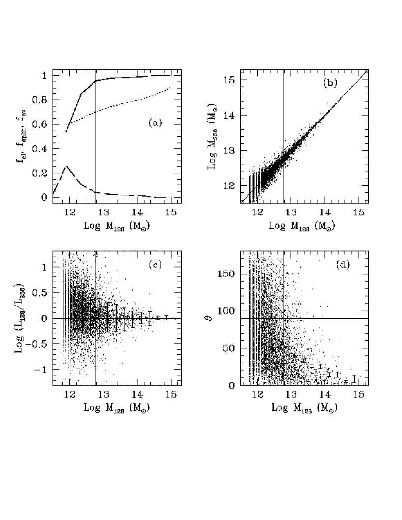
Figure 16: In all the panels the vertical line marks groups of 100 particles in the $\Lambda$CDM128 simulation. (a) Matching of the $\Lambda$CDM and $\Lambda$CDM128 halo catalogues. Continuous line: $f_{\rm cl}$; dashed line: $f_{\rm split}$; dotted line: $f_{\rm ov}$. (b) Correlation of masses for the cleanly assigned objects.(c) Fractional difference of angular momenta for the cleanly assigned objects, as a function of mass. Error bars give the rms difference in bins of mass. (d) Alignment angle between the angualr momenta of cleanly assigned objects. Error bars give the rms of the mean of the alignment angles in bins of mass.

Conversely, the error on the spin estimate turns out to be much larger. Figure 16c shows the fractional difference between halo spins as a function of mass (the rms difference is also shown), while figure 16d shows the alignment angles of the spins (the rms of the mean is shown in this case, as in figure 14). The rms difference is still in excess of a a factor of two for halos of 100 particles, and even larger for smaller halos. Moreover, the spin directions of small halos are very poorly correlated for halos with less than 100 particles. We conclude that the lower limit for a correct order-of-magnitude estimate of the angular momentum of a halo is 100 particles, while a more precise estimate will require at least ten times more particles.

References

- [] Antonuccio-Delogu V., Becciani U., Pagliaro A., van Kampen E., Colafrancesco S., Germanà A., Gambera M., 2001, MNRAS, in press (astro-ph/0009495)
- [] Audit E., Teyssier R., Alimi J.M.,1997, A&A, 325, 439
- [] Bardeen J.M., Bond J.R., Kaiser N., Szalay A.S., 1986, ApJ, 304, 15
- [] Barnes J., Efstathiou G. P., 1987, ApJ, 319, 575
- [] Benson A.J., Cole S., Frenk C.S., Baugh C.M., Lacey C.G,. 2000, MNRAS, 311, 793
- [] Bertschinger E., Jain B., 1994, ApJ, 431, 486
- [] Bode P., Bahcall N.A., Ford E.B., Ostriker J.P., 2000, submitted to ApJ (astro-ph/0011376)
- [] Bond J.R., Cole S., Efstathiou G., Kaiser N., 1991, ApJ, 379, 440
- [] Bond J.R., Myers S.T., 1996a, ApJS, 103, 1
- [] Bond J.R., Myers S.T., 1996b, ApJS, 103, 41
- [] Borgani S., Coles P., Moscardini L., 1994, MNRAS, 271, 223
- [] Bouchet F., 1996, in Dark Matter in the Universe, ed. S. Bonometto et al. IOS, Amsterdam
- [] Buchert T., 1992, A&A, MNRAS, 254, 729
- [] Buchert T., 1996, in Dark Matter in the Universe, ed. S. Bonometto et al. IOS, Amsterdam
- [] Buchert T., Ehlers J., 1993, MNRAS 264, 375
- [] Bullock J.S., Dekel A., Kolatt T.S., Kravtsov A.V., Klypin A.A., Porciani A., Primack J.R., 2001, ApJ, 555, 240
- [] Catelan P., 1995, MNRAS, 276, 115
- [] Catelan P., Lucchin F., Matarrese S., Porciani C., 1998, MNRAS, 297, 692
- [] Catelan P., Theuns T., 1996a, MNRAS, 282, 436
- [] Catelan P., Theuns T., 1996b, MNRAS, 282, 455
- [] Cavaliere A., Colafrancesco S., Menci N., 1992, ApJ, 392, 41
- [] Cavaliere A., Menci N., Tozzi P., 1996, ApJ, 464, 44
- [] Cole S., Kaiser N., 1988, MNRAS, 233, 637
- [] Cole S., Lacey C.G., 1996, MNRAS, 281, 716
- [] Cole S., Lacey C.G., Baugh C.M., Frenk C.S., 2000, MNRAS, 319, 168
- [] Coles P. Melott A.L., Shandarin S.F., 1993, MNRAS, 260, 765
- [] Couchman H., Thomas P., Pearce F., 1995, ApJ 452 797
- [] iaferio A., Kauffmann G., Colberg J.M., White S.D.M., 1999, MNRAS, 307, 537
- [] Efstathiou, G., Frenk, C.S., White, S.D.M., Davis, M., 1988, MNRAS, 235, 715
- [] Eisenstein D.J., Hut P., 1998, ApJ, 498, 137
- [] Gardner J.P., 2001, ApJ, 557, 616
- [] Governato F., Babul A., Quinn T., Tozzi P., Baugh C.M., Katz N., Lake G., 1999, MNRAS, 307, 949
- [] Hanami H., 1999, submitted to MNRAS (astro-ph/9910033)
- [] Heavens A., Peacock J., 1988, MNRAS, 232, 339
- [] Hoyle F., 1949, in Burgers J.M., van der Hulst H.C., eds., Problems of Cosmical Aerodynamics, Central Air Document Office, Dayton. p. 195
- [] Jenkins A., Frenk C.S., White S.D.M., Colberg J.M., Cole S., Evrard A.E., Couchman H.M.P., Yoshida N., 2001, MNRAS, 321, 372
- [] Kerscher M., Buchert T., Futamase T., 2000, submitted to ApJ (astro-ph/0007284)
- [] Lacey C., Cole S., 1993, MNRAS, 262, 627
- [] Lacey C., Cole S., 1994, MNRAS, 271, 676
- [] Lanzoni B., Mamon G.A., Guiderdoni B., 2000, MNRAS, 312, 781
- [] Lemson G., Kauffmann G., 1998, MNRAS, 302, 111
- [] Lee J., Shandarin S.F., 1998, ApJ, 500, 14
- [] Maller A.H., Dekel A., Somerville R.S., 2001, MNRAS, in press (astro-ph/0105168)
- [] Manrique A., Salvador-Solé E., 1995, ApJ, 453, 6
- [] Mo H., White S.D.M., 1996, MNRAS, 282, 189
- [] Mo H., Mao S., White S. D. M., 1998, MNRAS, 295, 319
- [] Monaco P., 1995, ApJ, 447, 23
- [] Monaco P., 1997a, MNRAS, 287, 753
- [] Monaco P., 1997b, MNRAS, 287, 753
- [] Monaco P., 1998, Fund. Cosm. Phys., 19, 153
- [] Monaco P., 1999, in Observational Cosmology: the development of galaxy systems, ed. G. Giuricin, M. Mezetti & P. Salucci. ASP Conf. Ser. 176. Pag. 186
- [] Monaco P., Murante G., 1999, Phys. Rev. D, 60, 0635XX
- [] Monaco P., Theuns T., Taffoni G., Governato F., Quinn T., Stadel J., 2001, ApJ, in press (paper I)
- [] Moutarde F.,Alimi J. M. ,Bouchet F. R.,Pellat R., Ramani A., 1991, ApJ 382, 377
- [] Nagashima M., Gouda N., 1998, MNRAS, 301, 849
- [] Padmanabhan T., 1993, Structure Formation in the Universe. Cambridge University Press
- [] Peacock J. A. Heavens A. F., 1985, MNRAS, 217, 805
- [] Peacock J. A. Heavens A. F., 1990, MNRAS, 243, 133
- [] Peebles P.J.E., 1993, Principles of Physical Cosmology, Princeton Univeristy Press, Princeton
- [] Porciani C., Catelan P., Lacey C., 1999, ApJ, 513, L99
- [] Porciani C., Dekel A., Hoffmann Y., 2001a, MNRAS, in press (astro-ph/0105123)
- [] Porciani C., Dekel A., Hoffmann Y., 2001b, MNRAS, in press (astro-ph/0105165)
- [] Press W.H., Schechter P., 1974, ApJ, 187, 425
- [] Rodrigues D.D.C., Thomas P.A., 1996, MNRAS, 282, 631
- [] Scoccimarro R., Sheth R.K., 2001, submitted to MNRAS (astro-ph/0106120)
- [] Shandarin S.F., Zel’dovich Ya.B.,1989, Rev. Mod. Phys., 61, 185
- [] Sheth R.K., Lemson G., 1999, MNRAS, 305, 946
- [] Sheth R.K., Mo H., Tormen G., 2001, MNRAS, in press
- [] Sheth R.K., Tormen G., 1999, MNRAS, 308, 119
- [] Sheth R.K., Tormen G., 2001, MNRAS, in press (astro-ph/0105113)
- [] Somerville R.S., Kolatt T.S., 1999, MNRAS, 305, 1
- [] Somerville R.S., Primack J.R., 1999, MNRAS, 310, 1087
- [] Taffoni G., Monaco P., Theuns T., 2001, MNRAS, submitted
- [] Theuns T., Leonard A., Efstathiou G., Pearce F.R., Thomas P.A., 1998, MNRAS, 301, 478
- [] Theuns T., Taffoni G., Monaco P., 2001, submitted to MNRAS
- [] Ueda H., Shimasaku K., Suginohara T., Suto Y., 1994, PASJ, 46, 319
- [] Vitvitsaka M., Klypin A.A., Kravtsov A.V., Bullock J.S., Wechsler R.H., Primack J.R., astro-ph/0105349
- [] White S.D.M., 1984, ApJ, 286, 38
- [] White S.D.M., 1996, in Schaeffer R. et al., eds, Cosmology & Large-scale structure, Proc. 60th Les Houches School, Elsevier, p. 349
- [] White S.D.M., Frenk C.S., 1991, ApJ, 379, 52
- [] White S.D.M., Silk J., 1979, ApJ, 232, 1
- [] Zel’dovich YA. B., 1970, Astrofizika, 6, 319 (translated in Astrophysics, 6, 164 [1973])