Bounds on the possible evolution of the Gravitational Constant
from Cosmological Type-Ia Supernovae

Abstract

Recent high-redshift Type Ia supernovae results can be used to set new bounds on a possible variation of the gravitational constant $G$. If the local value of $G$ at the space-time location of distant supernovae is different, it would change both the kinetic energy release and the amount of ⁵⁶Ni synthesized in the supernova outburst. Both effects are related to a change in the Chandrasekhar mass $M_{\rm Ch}\propto G^{-3/2}$. In addition, the integrated variation of $G$ with time would also affect the cosmic evolution and therefore the luminosity distance relation. We show that the later effect in the magnitudes of Type Ia supernovae is typically several times smaller than the change produced by the corresponding variation of the Chandrasekhar mass. We investigate in a consistent way how a varying $G$ could modify the Hubble diagram of Type Ia supernovae and how these results can be used to set upper bounds to a hypothetical variation of $G$. We find $G/G_{0}\mathrel{\mathchoice{\lower 3.6pt\vbox{\halign{$\mathsurround=0pt\displaystyle\hfill#\hfil$\cr<\crcr\sim\crcr}}}{\lower 3.6pt\vbox{\halign{$\mathsurround=0pt\textstyle\hfill#\hfil$\cr<\crcr\sim\crcr}}}{\lower 3.6pt\vbox{\halign{$\mathsurround=0pt\scriptstyle\hfill#\hfil$\cr<\crcr\sim\crcr}}}{\lower 3.6pt\vbox{\halign{$\mathsurround=0pt\scriptscriptstyle\hfill#\hfil$\cr<\crcr\sim\crcr}}}}1.1$ and $\dot{G}/G\mathrel{\mathchoice{\lower 3.6pt\vbox{\halign{$\mathsurround=0pt\displaystyle\hfill#\hfil$\cr<\crcr\sim\crcr}}}{\lower 3.6pt\vbox{\halign{$\mathsurround=0pt\textstyle\hfill#\hfil$\cr<\crcr\sim\crcr}}}{\lower 3.6pt\vbox{\halign{$\mathsurround=0pt\scriptstyle\hfill#\hfil$\cr<\crcr\sim\crcr}}}{\lower 3.6pt\vbox{\halign{$\mathsurround=0pt\scriptscriptstyle\hfill#\hfil$\cr<\crcr\sim\crcr}}}}10^{-11}{\rm yr}^{-1}$ at redshifts $z\simeq 0.5$. These new bounds extend the currently available constrains on the evolution of $G$ all the way from solar and stellar distances to typical scales of Gpc/Gyr, i.e. by more than 15 orders of magnitudes in time and distance.

]

I Introduction

One of the most important challenges of modern physics is the quantization of the gravitational force. The undergoing attempts to create such theories has re-opened the subject of varying fundamental constants. To this regard it is worth noticing that the constancy of the fundamental constants, and of the gravitational constant in particular, has been questioned for a long time [1, 2, 3, 4, 5] and that early attempts to unify gravity with electromagnetism [6, 7] predicted such kind of variations. Although modern theories, like the string theory and the M-theory (see [8] for a recent review), do not necessarily require a variation of the fundamental constants they provide a natural and self-consistent framework for such variations (see [9] and [10] for excellent descriptions of the theoretical background). As a general result, modern theories predict that in the ordinary three-dimensional subspace, gauge couplings like the fine structure constant $\alpha$ or the gravitational constant $G$ should vary as the inverse square of the mean scale of the extra dimensions. Hence, the evolution of the scale size of the additional dimensions is related to the variation of fundamental constants [11, 12, 13]. Moreover it has been recently shown [13] that a cosmological variation of $\alpha$ may proceed at different rates at different locations in space-time. The way in which the time variations of $\alpha$ and $G$ are linked is model dependent but a typical relation is: $\Delta\alpha/\alpha^{2}\sim\Delta G/G$. There have been several attempts to measure the rate of variation of $\alpha$, providing different results for different look-back times. For instance, [14] used the recently released CMB anisotropy data to set up early-universe constraints on a time-varying $\alpha$ and found no evidence for such a change, whereas [10, 15] used high resolution spectroscopy of QSO absorption systems to find statistical evidences for a smaller $\alpha$ at a redshift range $0.5<z<3.5$. Of course, since a cosmological variation of $\alpha$ (and, consequently, of $G$) can proceed at different rates for different redshifts [13] both studies are not necessarily in conflict. There have been also many attempts to measure a time variation of the gravitational constant which will be discussed later in §V. For the moment it is important to mention here that most of these bounds come either from local measurements (the sun, our solar system or the solar neighborhood) or from very early times measurements (namely Big-Bang nucleosynthesis), whereas at intermediate look-back times there are not such measurements.

Type Ia supernovae (SNIa) are supposed to be one of the best examples of standard candles. This is because, although the nature of their progenitors and the detailed mechanism of explosion are still the subject of a strong debate, their observational light curves are relatively well understood and their individual intrinsic differences can be accounted for. Under these assumptions, thermonuclear supernovae are well suited objects to study the Universe at large, especially at high redshifts $(z\sim 1.0)$, where the rest of standard candles fail in deriving reliable distances, thus providing an unique tool for determining cosmological parameters or discriminating among different alternative cosmological theories.

Using the observations of high redshift Type Ia supernovae $(z>0.1)$ and low redshift $(z<0.1)$ supernovae, both the Supernova Cosmology Project [16] and the High-$z$ Supernova Search Team [17] found that the peak luminosities of distant supernovae appear to be $\sim 0.20$ magnitude fainter than predicted for an empty universe and 0.25 magnitude fainter than predicted by a standard decelerating universe, with a presumed mass density $\Omega_{M}\simeq 0.3$. To be more precise, at the $1\sigma$ confidence level, the results of both groups can be well approximated by the relation:

$$0.8\,\Omega_{M}-0.6\,\Omega_{\Lambda}=-0.2\pm 0.1.$$ (1)

However these conclusions rely on the assumption that there is no mechanism able to produce an evolution of the observed light curves over cosmological distances. In other words: both teams assumed that the relation between the intrinsic peak luminosity and the time scales of the light curve were exactly the same for both the low-$z$ and the high-$z$ supernovae. The possible consequences for evolutionary effects in SNIa due to changes in the zero age mass and metalicity of the progenitor star have been explored by several authors [18, 19, 20], who found that changes in the underlying population cause a change in the maximum brightness by about 0.1-0.2 magnitudes.

The SNIa results have already motivated a significant number of papers that search for bounds on the variation in fundamental constants [21, 22, 23, 24, 25] or new cosmological scenarios, such as quintessence models [26] and scalar-field cosmologies [27]. This burst of interest is due to the conceptual problems that arise from infering the existence of a cosmological constant $\Lambda\simeq 10^{-122}c^{3}/G/\hbar$ or facing the cosmic (dark) matter problem (see [28] and references therein). There have been many suggestions that the apparent complications that arise can be eliminated by modifying the laws of gravity [29, 30, 31, 32, 33, 34, 35, 36].

Recent cosmological observations, such as the lastest CMB Boomerang and Maxima data [37, 38] indicate a flat Universe: $\Omega_{R}=0$, i.e. $\Omega_{M}+\Omega_{\Lambda}=1$. This result, together with the above equation 1 points in the direction of a non-cero $\Lambda$, although other interpretations are also possible [39, 40].

The purpose of this paper is to analyze the effect of varying $G$ in the current interpretation of the Hubble diagram of distant SNIa and to use this analysis to set upper bounds on its rate of change. The paper is organized as follows: in §II we describe the effects of a varying $G$ on the physics of supernovae; in §III and in the Appendix, we analyze the effects of a varying $G$ on the luminosity distance of distant supernovae. In §IV we present a likelihood analysis of the SNIa data which is then used to set upper bounds in the evolution of $G$. Finally in section V we discuss our results and draw our conclusions.

II The effects of a varying $G$ on the physics of supernovae

Simple analytical models of light curve (see, for instance, [41]) predict that the peak luminosity is proportional to the mass of nickel synthesized, which in turn, to a good approximation, is a fixed fraction of the Chandrasekhar mass $(M_{\rm Ni}\propto M_{\rm Ch})$, which depends on the value of gravitational constant as: $M_{\rm Ch}\propto G^{-3/2}$. The actual fraction varies when different specific SNIa scenarios are considered (e.g. [42, 43]), but the physical mechanisms relevant for type Ia supernovae naturally relates the energy yield to the Chandrasekhar mass. Here we will only focus on Chandrasekhar mass models since there are growing evidences that the sub-Chandrasekhar mass models do not fit well the observations (see, for instance, [44]). In summary, whatever the actual scenario is, we will assume that the same mechanism for the ignition and the propagation of the burning front is valid for SNIa at high and low redshifts. Thus, since the peak luminosity is proportional to the total amount of nickel synthesized in the supernova outburst we have $L\propto G^{-3/2}$, and, therefore, for a slow decrease of $G$ with time, distant supernovae should be dimmer than predicted for a standard scenario. Under this assumptions, we have:

$$M-M_{0}=\frac{15}{4}\log\Big{(}\frac{G}{G_{0}}\Big{)}$$ (2)

where $M$ stands, as usual, for the absolute magnitude, $G$ for the precise value of the gravitational constant at a given redshift and the subscript 0 denotes their local values. Note that the above equation does not require knowledge of the (unknown) proportionality constant relating the supernova luminosity with the Chandrasekhar mass. This dependence factorizes out under the assumptions above, and the final differential result is only sensitive to the values of $G$. From this equation we can see that in order to reduce the apparent luminosity of distant supernovae by $\Delta m\simeq 0.2$ a dramatic change of $G$ is required: $G/G_{0}\simeq 1.13$. This value should be regarded as an upper bound in the sense that part or all of the $\Delta m\simeq 0.2$ difference found by [16, 17] could be attributable to the hypothesis of an accelerating universe.

In order to test the validity of our argument we have computed a series of models of Type Ia supernovae explosion and their corresponding light curves, according to the procedure described in [45] and references therein, with the present local value of $G$, 1.1 and 1.2 times this value. The explosion model was a delayed detonation starting from a central density of $2.0\times 10{{}^{9}}\,{\rm g/cm}^{3}$ a core temperature of $2.0\times 10^{8}$ K and making the transition from deflagration to detonation when the flame density went below $2.0\times 10^{7}\,{\rm g/cm}^{3}$. Our study is based on delayed detonation models, because these have been found to reproduce the optical and infrared light curves and spectra of Type Ia supernovae reasonably well [19, 46, 47, 48, 49, 50, 51]. The model parameters, ignition density and transition density, are those that allow us to reproduce a typical Type Ia Supernovae. The results are shown in Table 1 and Figure 1.

FIG. 1.: Bolometric light curves of SNIa for the local value of the gravitational constant, $G_{0}$ (solid line), for $G_{1}=1.1G_{0}$ (dotted line) and for $G_{1}$ shifted upwards by 0.18 magnitudes. See text for details.

In Table 1 we show the mass of the white dwarf model in hydrostatic equilibrium from which the explosion was computed, $M_{\rm WD}$, the kinetic energy, $K$, the mass of synthesized nickel, $M_{\rm Ni}$, the peak bolometric magnitude, $M_{\rm bol}^{\rm peak}$, and a measure of the width of the light curve, $\Delta m_{15}$ — see below for a precise definition. All the masses are expressed in solar units. In Figure 1 we show the light curves for $G/G_{0}=1.0$ — solid line — $G_{1}=G/G_{0}=1.1$ — dotted line — and this last light curve shifted upwards by a constant amount of 0.18 magnitudes — dashed-dotted line — in accordance with the behavior predicted by Eq.[2].

As it can be seen in Table 1 the simple energetic argument presented above is in good agreement with the detailed calculations presented here and, thus, the energy liberated in the supernova outburst indeed scales as $G^{-3/2}$. Hence, the bolometric magnitude at the peak of the light curve computed with a larger value of $G$ should be moved upwards by a fixed constant amount which depends on the exact value of $G$. Figure 1 clearly shows this behavior. It should be stressed at this point that our analysis does not depend on the detailed physics of Type Ia supernovae since the functional dependence on the Chandrasekhar mass comes from basic physical arguments and it is unavoidable, no matter which are the (unknown) details of the explosion unless we change the physics underlaying the Chandrasekhar mechanism.

Figure 1 also shows that once this vertical shift is done, the duration of the supernova outburst is also modified by a varying $G$, being the decline faster for the models with larger $G$, especially at late times. As it can be seen there, in the region near the maximum (see the insert for a close up of this region) the difference between both light curves is small when due account of the vertical shift is done. A good parameterization of the slope (and, thus, of the width) of the light curve is $\Delta m_{15}$, which is defined as the difference in the apparent magnitude 15 days after the maximum. It turns out that the maximum of the light curve for the models presented in Fig. 1 occurs at 13.0 and 12.5 days, being $\Delta m_{15}=0.85$ and 0.89, respectively. This, in turn, implies that since the template light curve used to calibrate the distances to distant supernovae takes into account the width of the light curve, and in particular $\Delta m_{15}$ is used, a variation of the gravitational constant should ultimately affect as well the final value of the derived distances. However, given the slight variation of the $\Delta m_{15}$ parameter this can be clearly considered as a second order effect. Nevertheless, as it can be clearly seen in Fig. 1, although there is not any large difference in the rise-times or in the early time light curve due to a varying $G$ there is indeed an appreciable difference in the overall duration of the supernova event. To be precise the widths at $M_{\rm bol}=-16$ are 126 and 112 days, respectively.

This result can be interpreted in terms of very simple physical considerations, and in particular, in terms of the simplified model of light curve presented in [41] which has a reasonable accuracy (of the order of $\sim 20$%). According to this analytic model of light curve, the width of the peak of the light curve of SNIa is given by:

TABLE I.: Overall characteristics of the supernova explosion for several values of $G$, and the same ignition density.

$G/G_{0}$	$M_{\rm WD}$	$K/10^{51}\,{\rm erg}$	$M_{\rm Ni}$	$M_{\rm bol}^{\rm peak}$	$\Delta m_{15}$
1.0	1.37	1.34	0.69	$-19.43$	0.85
1.1	1.19	1.14	0.57	$-19.25$	0.89
1.2	1.04	0.95	0.49	$-19.13$	0.91

$$\tau\propto\Big{(}\frac{M_{\rm ej}^{3}}{K}\Big{)}^{1/4}$$ (3)

where $M_{\rm ej}$ is the ejected mass and $K$ is the kinetic energy. Within our current knowledge of the mechanisms of explosion of SNIa both the ejected mass and the supernova kinetic energy can be considered proportional to the Chandrasekhar mass, and therefore we have $\tau\propto M_{\rm Ch}^{1/2}$ or, equivalently, $\tau\propto G^{-3/4}$. Thus we have

$$\Big{\langle}\frac{\tau}{\tau_{0}}\Big{\rangle}\simeq\Big{\langle}\frac{G}{G_{0}}\Big{\rangle}^{-3/4}.$$ (4)

The ratio of the durations of the supernova outburst calculations presented above matches reasonably well the behavior predicted by Eq.[4]. Hence, in the case in which a varying gravitational constant is considered, the overall time scales of the supernovae light curves should depend as well on the actual value of $G$.

It has been recently claimed that there is a mean evolution in the rise-times of local and distant supernovae [52, 53]. In particular the widths of the light curve when the supernova is 2.5 magnitudes fainter than the peak luminosity was found to be $\tau_{0}=45.0\pm 0.15$ (at $z\simeq 0$) and $\tau=43.8\pm 0.40$ days (at $z\simeq 0.5$), were the errors in the widths were ascribed solely to the errors in the rise-times. Using this data and Eq.[4], [23] obtained $G/G_{0}\leq 1.037\pm 0.017$ ($2\sigma$ errors) at $z\simeq 0.5$, a variation of $G$ very similar to the one needed to explain the change in the peak luminosity. Subsequent studies [54] have demonstrated that the rise-times of local and distant supernovae are consistent each another and that the rise-time uncertainties were underestimated, being revised upwards to $\pm 1.2$ days statistical and ${}^{+3.6}_{-1.9}$ days due to systematical bias under extreme situations. According to this last analysis there is still some room for deviations of the light curve of high redshift supernovae at late times. This is exactly what we have found. However, it is worth mentioning at this point that according to this study these late time deviations systematically influence the rise-time determinations. Conversely, should we have tried to fit the late time light curve we would have found a significant difference in the corresponding rise-times. In the light of this new analysis, there is no significant evidence for a possible change in $G$. For our purposes, since the situation is not yet clear from the observational point of view our analysis will only rely on the limits imposed by Eq.[2]. Note however that, on the other hand, should a firm estimate of the maximum value of the difference between the local and distant supernovae timescales could be eventually obtained a very stringent upper limit to the rate of variation of the gravitational constant would be derived, which, additionally, would not depend on the adopted cosmological model but on the well calibrated relation between the duration of the supernova outburst and its peak magnitude.

III The Hubble diagram

The next question we want to address here is how an hypothetical variation of the gravitational constant (of the amount of a few percent) translates in the Hubble diagram of distant supernovae. In addition to the change in the intrinsic energy release and of the duration of the supernova event induced by the variation in the Chandrasekhar mass, the integrated evolution of $G$ with time would also affect the cosmic evolution and, therefore, the luminosity distance relation. To make this quantitative we need to consider non-standard cosmological models. It is however beyond the scope of this paper to discuss specific theoretical models to replace the standard theory of General Relativity. This has been discussed in detail elsewhere in the literature [55, 56, 57, 58, 59, 60], and also in the context of an accelerating universe [35, 61, 62, 63].

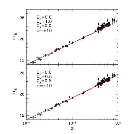
FIG. 2.: Hubble diagrams for the high-redshift SNIa data with different choices of cosmological parameters and different values of $\dot{G}$ . Continuous lines correspond to the standard cosmology with $G(z)=G_{0}$. Dashed lines bracket the effects on the peak luminosity from a $\simeq 5\%$ variation in $G$. The observational data has been obtained from [16].

In the appendix we show in a self-consistent way that for plausible models which incorporate a varying $G$, such as scalar-tensor theories (STTs), the possible effect of a varying $G$ on the cosmological evolution gives a contribution to the luminosity distance relation at the distances of interest which is several times smaller than the effect produced by the same variation of $G$ on the Chandrasekhar mass. We will therefore concentrate our analysis on the effects of the physics of the supernovae. This complements the analysis of [35, 62, 63] which neglected the effects in the physics of the supernovae and used the evidence for the accelerating universe as a way to constraint cosmic evolution in non-standard theories of gravity.

In analogy to STTs, we will parameterize the evolution of $G$ in terms of the strength of coupling parameter, $\omega$, as:

$$G(z)\equiv G_{0}(1+z)^{1\over{1+\omega(z)}},$$ (5)

which provides our definition for $\omega(z)$ — see the appendix for further details. Thus a value of $\omega\simeq 10$ produces a $\simeq 4\%$ increase in $G$ at $z\simeq 0.5$, while $\omega\simeq-10$ produces a $\simeq 5\%$ decrease in $G$ at $z\simeq 0.5$. In summary, Eq.[5] gives the change in $G$ as a function of $\omega$ while Eq.[A3-A5] give the corresponding cosmic evolution. Thus we have:

$$m(z)=M_{0}+5~{}\log d_{L}+25+\frac{15}{4(1+\omega)}\log\big{(}1+z\big{)}$$ (6)

where $d_{L}=d_{L}(z,\Omega_{M},\Omega_{\Lambda})$ is obtained from the line-of-sight comoving distance (see the appendix). For illustrative purposes Figure 2 shows the above relation for two representative cosmological models, including the effects of $\omega$ in $d_{L}$, for $\omega=\pm 10$ (dotted lines), which correspond to a change of $G$ of $\sim 5\%$, and the standard $(\omega=\infty)$ case (solid line).

IV Bounds on $\dot{G}/G$

We have re-done the likelihood analysis of the Supernova Cosmology Project allowing for a varying $G$. Thus, we use the same observational data but with the magnitude-distance relation given by Eq.[6]. Here we have one extra function $\omega(z)$ to be fitted. At low redshifts the last term in the r.h.s. of Eq.[6] has a negligible contribution. Given that most of the SNIa at high redshift cluster around $z\simeq 0.5$ and that we are expecting $\omega$ to be large (so that $G\simeq G_{0}$ in Eq.[5]), the effect of $\omega(z)$ in the fit to Eq.[6] is dominated by the value of $\omega$ at the mean redshift of the SNIa sample, $z\simeq 0.5$. Hence, we can approximate $\omega(z)\simeq\omega(z\simeq 0.5)$ and fit the data as a function of this new extra parameter, $\omega(z\simeq 0.5)$ or $G(z\simeq 0.5)/G(z\simeq 0)\equiv G/G_{0}$.

Our results are plotted in Figures 3 and 4, where we show the confidence contours (at the 99%, 90%, 68% — solid lines — 5% and 1% confidence level — dotted lines) obtained from the fit to the Hubble diagram of SNIa. Figure 3 shows the likelihood contours for $G/G_{0}\equiv G(z\simeq 0.5)/G(z\simeq 0)$ as a function of $\Omega_{\Lambda}$ for a flat $\Omega_{R}=0$ universe, whereas Figure 4 shows the likelihood contours in the $(G/G_{0},\Omega_{M})$ plane for the case $\Omega_{\Lambda}=0$. As it can seen in these figures, the expected departures from the standard case $(G/G_{0}\simeq 1)$ are quite small for a reasonable choice of cosmological parameters. This, in turn, justifies our approximation $\omega(z)\simeq\omega(z\simeq 0.5)$. It is also worth mentioning at this point that we have also tried linear fits to $\omega(z)\simeq\omega_{0}+\omega^{\prime}z$ and found equivalent results.

FIG. 3.: Confidence contours for the best fit SNIa data in the plane $(G/G_{0},\Omega_{\Lambda})$ for a flat universe $\Omega_{R}=0$.

FIG. 4.: Confidence contours for the best fit SNIa data in the plane $(G/G_{0},\Omega_{M})$ for $\Omega_{\Lambda}=0$.

The confidence intervals of these figures can be used to set bounds in $G/G_{0}$. These are bounds in the sense that, given a cosmological model, we assume that all the difference in SNIa corrected peak luminosities can be attributed solely to a difference in Chandrasekhar mass. For example, for the flat $\Omega_{\Lambda}\simeq 0$ model we have at 1$\sigma$ confidence level:

$${G\over{G_{0}}}\mathrel{\mathchoice{\lower 3.6pt\vbox{\halign{$\mathsurround=0pt\displaystyle\hfill#\hfil$\cr<\crcr\sim\crcr}}}{\lower 3.6pt\vbox{\halign{$\mathsurround=0pt\textstyle\hfill#\hfil$\cr<\crcr\sim\crcr}}}{\lower 3.6pt\vbox{\halign{$\mathsurround=0pt\scriptstyle\hfill#\hfil$\cr<\crcr\sim\crcr}}}{\lower 3.6pt\vbox{\halign{$\mathsurround=0pt\scriptscriptstyle\hfill#\hfil$\cr<\crcr\sim\crcr}}}}1.2~{}~{};~{}~{}\Omega_{\Lambda}\simeq 0.0~{},~{}\Omega_{M}\simeq 1.0,$$ (7)

while for the flat $\Omega_{\Lambda}\simeq 0.8$ case

$${G\over{G_{0}}}\mathrel{\mathchoice{\lower 3.6pt\vbox{\halign{$\mathsurround=0pt\displaystyle\hfill#\hfil$\cr<\crcr\sim\crcr}}}{\lower 3.6pt\vbox{\halign{$\mathsurround=0pt\textstyle\hfill#\hfil$\cr<\crcr\sim\crcr}}}{\lower 3.6pt\vbox{\halign{$\mathsurround=0pt\scriptstyle\hfill#\hfil$\cr<\crcr\sim\crcr}}}{\lower 3.6pt\vbox{\halign{$\mathsurround=0pt\scriptscriptstyle\hfill#\hfil$\cr<\crcr\sim\crcr}}}}1.08~{}~{};~{}~{}\Omega_{\Lambda}\simeq 0.8~{},~{}\Omega_{M}\simeq 0.2$$ (8)

also at $1\sigma$ confidence level. In terms of the $\omega\simeq\omega(z\simeq 0.5)$ parameter these later bounds translate into $\omega\mathrel{\mathchoice{\lower 3.6pt\vbox{\halign{$\mathsurround=0pt\displaystyle\hfill#\hfil$\cr>\crcr\sim\crcr}}}{\lower 3.6pt\vbox{\halign{$\mathsurround=0pt\textstyle\hfill#\hfil$\cr>\crcr\sim\crcr}}}{\lower 3.6pt\vbox{\halign{$\mathsurround=0pt\scriptstyle\hfill#\hfil$\cr>\crcr\sim\crcr}}}{\lower 3.6pt\vbox{\halign{$\mathsurround=0pt\scriptscriptstyle\hfill#\hfil$\cr>\crcr\sim\crcr}}}}1.2$ for $\Omega_{\Lambda}\simeq 0$ and $\omega\mathrel{\mathchoice{\lower 3.6pt\vbox{\halign{$\mathsurround=0pt\displaystyle\hfill#\hfil$\cr>\crcr\sim\crcr}}}{\lower 3.6pt\vbox{\halign{$\mathsurround=0pt\textstyle\hfill#\hfil$\cr>\crcr\sim\crcr}}}{\lower 3.6pt\vbox{\halign{$\mathsurround=0pt\scriptstyle\hfill#\hfil$\cr>\crcr\sim\crcr}}}{\lower 3.6pt\vbox{\halign{$\mathsurround=0pt\scriptscriptstyle\hfill#\hfil$\cr>\crcr\sim\crcr}}}}4.3$ for $\Omega_{\Lambda}\simeq 0.8$. It is important to mention here that these constraints are quite loose when compared with the bounds on $\omega$ from very long baseline interferometry in the local Universe, $\omega_{0}>2600$, [60], but, on the other hand, are new in the sense that they correspond to an earlier (or equivalently more distant) Universe. Moreover, the SNIa data provide more interesting limits to $\dot{G}/G$. To obtain them we can use

$${\dot{G}\over G}\simeq\left(1-{G_{0}\over{G}}\right)(\Delta t)^{-1}$$ (9)

where $\Delta t$ is the look-back time to $z\simeq 0.5$:

$$\Delta t=\int_{0}^{z}\frac{dz^{\prime}}{(1+z^{\prime})\,H(z^{\prime})}$$ (10)

with $H(z)$ given by Eq.[A3]. For a flat $\Omega_{\Lambda}\simeq 0$ model we have that $\Delta t\simeq 4.6\times 10^{9}{\rm yr}/h_{70}$ ($h_{70}$ is the Hubble constant in units of $H_{0}=70~{}{\rm Km/s/Mpc}$), while for the flat $\Omega_{\Lambda}\simeq 0.8$ case we have $\Delta t\simeq 6.0\times 10^{9}{\rm yr}/h_{70}$. Thus we find:

$${\dot{G}\over G}\mathrel{\mathchoice{\lower 3.6pt\vbox{\halign{$\mathsurround=0pt\displaystyle\hfill#\hfil$\cr<\crcr\sim\crcr}}}{\lower 3.6pt\vbox{\halign{$\mathsurround=0pt\textstyle\hfill#\hfil$\cr<\crcr\sim\crcr}}}{\lower 3.6pt\vbox{\halign{$\mathsurround=0pt\scriptstyle\hfill#\hfil$\cr<\crcr\sim\crcr}}}{\lower 3.6pt\vbox{\halign{$\mathsurround=0pt\scriptscriptstyle\hfill#\hfil$\cr<\crcr\sim\crcr}}}}36\times 10^{-12}~{}h_{70}/{\rm yr}~{}~{} ~{}~{}\Omega_{\Lambda}\simeq 0.0~{},~{}\Omega_{M}\simeq 1.0$$ ; (19)

$${\dot{G}\over G}\mathrel{\mathchoice{\lower 3.6pt\vbox{\halign{$\mathsurround=0pt\displaystyle\hfill#\hfil$\cr<\crcr\sim\crcr}}}{\lower 3.6pt\vbox{\halign{$\mathsurround=0pt\textstyle\hfill#\hfil$\cr<\crcr\sim\crcr}}}{\lower 3.6pt\vbox{\halign{$\mathsurround=0pt\scriptstyle\hfill#\hfil$\cr<\crcr\sim\crcr}}}{\lower 3.6pt\vbox{\halign{$\mathsurround=0pt\scriptscriptstyle\hfill#\hfil$\cr<\crcr\sim\crcr}}}}12\times 10^{-12}~{}h_{70}/{\rm yr}~{}~{} ~{}~{}\Omega_{\Lambda}\simeq 0.8~{},~{}\Omega_{M}\simeq 0.2$$ ; (28)

It should be stressed that these are bounds on ${\dot{G}/G}$ around $z\simeq 0.5$. Several local bounds on the rate of change of the gravitational constant, ${\dot{G}_{0}/G_{0}}$, have been obtained, for example, from binary pulsars, from the Viking Radar and from Lunar Laser Ranging, yielding typical upper bounds of ${\dot{G}_{0}/G_{0}}\mathrel{\mathchoice{\lower 3.6pt\vbox{\halign{$\mathsurround=0pt\displaystyle\hfill#\hfil$\cr<\crcr\sim\crcr}}}{\lower 3.6pt\vbox{\halign{$\mathsurround=0pt\textstyle\hfill#\hfil$\cr<\crcr\sim\crcr}}}{\lower 3.6pt\vbox{\halign{$\mathsurround=0pt\scriptstyle\hfill#\hfil$\cr<\crcr\sim\crcr}}}{\lower 3.6pt\vbox{\halign{$\mathsurround=0pt\scriptscriptstyle\hfill#\hfil$\cr<\crcr\sim\crcr}}}}10\times 10^{-12}{\rm yr}^{-1}$ (see, for instance, [60]). Other bounds come from the theory of stellar evolution, like white dwarf cooling [64], being the bounds of the order of $10\times 10^{-12}{\rm yr}^{-1}$. Finally, it should be mentioned that some other local bounds are as low as ${\dot{G}_{0}/G_{0}}<6\times 10^{-12}{\rm yr}^{-1}$ [65]. Note, however, that the values of all these bounds are comparable to that obtained here. Thus, despite the fact that the SNIa bounds on $G/G_{0}$ are quite loose, the longer time baseline obtained by using high redshift measurements puts stronger constraints on ${\dot{G}/G}$. These bounds on the change in $G$ correspond to redshifts which have not been explored yet in the more standard gravitational tests, mostly based on solar system and stellar physics. We can combine the SNIa and local bounds further to set a bound on $\ddot{G}$:

$${\ddot{G}\over G}\mathrel{\mathchoice{\lower 3.6pt\vbox{\halign{$\mathsurround=0pt\displaystyle\hfill#\hfil$\cr<\crcr\sim\crcr}}}{\lower 3.6pt\vbox{\halign{$\mathsurround=0pt\textstyle\hfill#\hfil$\cr<\crcr\sim\crcr}}}{\lower 3.6pt\vbox{\halign{$\mathsurround=0pt\scriptstyle\hfill#\hfil$\cr<\crcr\sim\crcr}}}{\lower 3.6pt\vbox{\halign{$\mathsurround=0pt\scriptscriptstyle\hfill#\hfil$\cr<\crcr\sim\crcr}}}}4\times 10^{-21}~{}(h_{70}/{\rm yr})^{2}$$ (29)

In terms of $\omega(z)$ we can also set some further limits by doing a Taylor expansion as in [62]:

$$\omega^{-1}\simeq\omega^{-1}_{0}+z\left|{d\omega^{-1}\over{dz}}\right|_{0}$$ (30)

so that we find:

$$\left|{d\omega^{-1}\over{dz}}\right|_{0}\mathrel{\mathchoice{\lower 3.6pt\vbox{\halign{$\mathsurround=0pt\displaystyle\hfill#\hfil$\cr<\crcr\sim\crcr}}}{\lower 3.6pt\vbox{\halign{$\mathsurround=0pt\textstyle\hfill#\hfil$\cr<\crcr\sim\crcr}}}{\lower 3.6pt\vbox{\halign{$\mathsurround=0pt\scriptstyle\hfill#\hfil$\cr<\crcr\sim\crcr}}}{\lower 3.6pt\vbox{\halign{$\mathsurround=0pt\scriptscriptstyle\hfill#\hfil$\cr<\crcr\sim\crcr}}}}1.7~{}~{} ~{}~{}\Omega_{\Lambda}\simeq 0.0~{},~{}\Omega_{M}\simeq 1.0$$ ; (39)

$$\left|{d\omega^{-1}\over{dz}}\right|_{0}\mathrel{\mathchoice{\lower 3.6pt\vbox{\halign{$\mathsurround=0pt\displaystyle\hfill#\hfil$\cr<\crcr\sim\crcr}}}{\lower 3.6pt\vbox{\halign{$\mathsurround=0pt\textstyle\hfill#\hfil$\cr<\crcr\sim\crcr}}}{\lower 3.6pt\vbox{\halign{$\mathsurround=0pt\scriptstyle\hfill#\hfil$\cr<\crcr\sim\crcr}}}{\lower 3.6pt\vbox{\halign{$\mathsurround=0pt\scriptscriptstyle\hfill#\hfil$\cr<\crcr\sim\crcr}}}}0.5~{}~{} ~{}~{}\Omega_{\Lambda}\simeq 0.8~{},~{}\Omega_{M}\simeq 0.2$$ ; (48)

Future experiments, such as the Supernovae Acceleration Probe (SNAP), could achieve a few percent magnitude errors up to redshifts of $z\simeq 1.7$ (see [66]). By then, we can also fairly assume that other observational data, such as the LSS and CMB experiments, will provide a knowledge of a few percent on the cosmological parameters [28]. Thus we can translate the uncertainty in the magnitude directly into bounds on $G$:

$$\Delta m\simeq\frac{15}{4}\log\Big{(}\frac{G}{G_{0}}\Big{)}.$$ (49)

Note that the possible effects of a varying $G$ on the luminosity distance discussed in the Appendix, are still several times smaller than the above contribution for $z\simeq 1.7$. For example, a $1\%$ uncertainty in $\Delta m$ (both from peak luminosity and cosmological parameter errors) will give us a $0.6\%$ bound in $G/G_{0}\mathrel{\mathchoice{\lower 3.6pt\vbox{\halign{$\mathsurround=0pt\displaystyle\hfill#\hfil$\cr<\crcr\sim\crcr}}}{\lower 3.6pt\vbox{\halign{$\mathsurround=0pt\textstyle\hfill#\hfil$\cr<\crcr\sim\crcr}}}{\lower 3.6pt\vbox{\halign{$\mathsurround=0pt\scriptstyle\hfill#\hfil$\cr<\crcr\sim\crcr}}}{\lower 3.6pt\vbox{\halign{$\mathsurround=0pt\scriptscriptstyle\hfill#\hfil$\cr<\crcr\sim\crcr}}}}1.006$ at $z\simeq 1.7$ or, equivalently, $\omega\mathrel{\mathchoice{\lower 3.6pt\vbox{\halign{$\mathsurround=0pt\displaystyle\hfill#\hfil$\cr>\crcr\sim\crcr}}}{\lower 3.6pt\vbox{\halign{$\mathsurround=0pt\textstyle\hfill#\hfil$\cr>\crcr\sim\crcr}}}{\lower 3.6pt\vbox{\halign{$\mathsurround=0pt\scriptstyle\hfill#\hfil$\cr>\crcr\sim\crcr}}}{\lower 3.6pt\vbox{\halign{$\mathsurround=0pt\scriptscriptstyle\hfill#\hfil$\cr>\crcr\sim\crcr}}}}167$. The later value is not particularly impressive as compared to the local bounds in the context of Jordan-Brans-Dicke (JBD) theories ($\omega>2500$). But note that $z\simeq 1.7$ corresponds to a look-back time in Eq.[10] as large as $\Delta t\simeq 10\times 10^{9}{\rm yr}/h_{70}$. Thus, future data would eventually yield firm bounds for $\dot{G}$ as low as:

$${\dot{G}\over G}\mathrel{\mathchoice{\lower 3.6pt\vbox{\halign{$\mathsurround=0pt\displaystyle\hfill#\hfil$\cr<\crcr\sim\crcr}}}{\lower 3.6pt\vbox{\halign{$\mathsurround=0pt\textstyle\hfill#\hfil$\cr<\crcr\sim\crcr}}}{\lower 3.6pt\vbox{\halign{$\mathsurround=0pt\scriptstyle\hfill#\hfil$\cr<\crcr\sim\crcr}}}{\lower 3.6pt\vbox{\halign{$\mathsurround=0pt\scriptscriptstyle\hfill#\hfil$\cr<\crcr\sim\crcr}}}}6\times 10^{-13}~{}h_{70}/{\rm yr}~{}~{};~{}~{}~{}z\simeq 1.7$$ (50)

which are more competitive than the current local values. The bounds to the change in $\omega$, could be reduced to:

$$\left|{d\omega^{-1}\over{dz}}\right|_{0}\mathrel{\mathchoice{\lower 3.6pt\vbox{\halign{$\mathsurround=0pt\displaystyle\hfill#\hfil$\cr<\crcr\sim\crcr}}}{\lower 3.6pt\vbox{\halign{$\mathsurround=0pt\textstyle\hfill#\hfil$\cr<\crcr\sim\crcr}}}{\lower 3.6pt\vbox{\halign{$\mathsurround=0pt\scriptstyle\hfill#\hfil$\cr<\crcr\sim\crcr}}}{\lower 3.6pt\vbox{\halign{$\mathsurround=0pt\scriptscriptstyle\hfill#\hfil$\cr<\crcr\sim\crcr}}}}3.5\times 10^{-3}~{}~{};~{}~{}z\simeq 1.7$$ (51)

Finally it is interesting to mention here that our analysis has been restricted to the peak magnitudes of supernovae. Comparable bounds can be found from the duration of supernovae events (Eq.[4]), if the statistical and systematic errors are reduced significantly, being the advantage of these last ones that are independent of the adopted cosmological model.

V Discussion and Conclusions

In astrophysics and cosmology the laws of physics (and in particular the simplest version of general relativity) are extrapolated outside its observational range of validity. It is therefore important to test for deviations of these laws at increasing cosmological scales and times (redshifts). SNIa provide us with a new tool to test how the laws of gravity and cosmology were in faraway galaxies ($z\simeq 0.5$). The observational limits on $\dot{G}/G$ come from quite different times and scales [58, 60, 67], but mostly in the local and nearby environments at $z\simeq 0$ (solar system, binary pulsars, and neutron stars [60]). There are also limits derived from the white dwarf cooling theory [64], which are based on similar arguments to the ones presented in this paper. Typical upper bounds give $\dot{G}/G\mathrel{\mathchoice{\lower 3.6pt\vbox{\halign{$\mathsurround=0pt\displaystyle\hfill#\hfil$\cr<\crcr\sim\crcr}}}{\lower 3.6pt\vbox{\halign{$\mathsurround=0pt\textstyle\hfill#\hfil$\cr<\crcr\sim\crcr}}}{\lower 3.6pt\vbox{\halign{$\mathsurround=0pt\scriptstyle\hfill#\hfil$\cr<\crcr\sim\crcr}}}{\lower 3.6pt\vbox{\halign{$\mathsurround=0pt\scriptscriptstyle\hfill#\hfil$\cr<\crcr\sim\crcr}}}}10^{-11}-10^{-12}$ yr^-1  [60].

Here we have proved by using detailed numerical models that if the value of $G$ at the space-time location of distant supernovae is different from the local one, it would change both the thermonuclear energy release and the time scale of the supernova outburst. The change can be quantified by means of the change in the Chandrasekhar mass $M_{\rm Ch}\propto G^{-3/2}$, and our detailed numerical results have been interpreted in terms of a very simple physical model. To this regard it is important to realize that our conclusions would remain unchanged should a modification of the parameters of the explosion lead to a smaller mass of ⁵⁶Ni synthesized in the supernova event, leading to a dimmer supernova.

We have also shown in a self-consistent way that for plausible models for a varying $G$, such as scalar-tensor theories, the possible effect of a varying $G$ on the cosmological evolution yields a contribution to the luminosity distance relation which is one order of magnitude smaller than the effect produced by the same variation of $G$ on the Chandrasekhar mass. Thus our approach complements the analysis of [35, 62, 63] which neglected the effects in the physics of the supernovae and used the evidence for the accelerating universe as a way to constraint cosmic evolution in non-standard theories of gravity.

In this paper we have also found further bounds for a varying $G$ from a likelihood analysis of the peak luminosities of the Supernova Cosmology Project. Our results are summarized in Figures 3 and 4 and Eq.[7]-[8], with values of $G/G_{0}\mathrel{\mathchoice{\lower 3.6pt\vbox{\halign{$\mathsurround=0pt\displaystyle\hfill#\hfil$\cr<\crcr\sim\crcr}}}{\lower 3.6pt\vbox{\halign{$\mathsurround=0pt\textstyle\hfill#\hfil$\cr<\crcr\sim\crcr}}}{\lower 3.6pt\vbox{\halign{$\mathsurround=0pt\scriptstyle\hfill#\hfil$\cr<\crcr\sim\crcr}}}{\lower 3.6pt\vbox{\halign{$\mathsurround=0pt\scriptscriptstyle\hfill#\hfil$\cr<\crcr\sim\crcr}}}}1.2$. We have further translated these results into bounds for $\dot{G}/G$ in Eq.[28], $\ddot{G}/G$ in Eq.[29] and ${d\omega^{-1}/{dz}}$ in Eq.[48]. Some of these bounds are new or comparable to other existing estimates from the local universe, which typically gives stronger constraints for $\omega$ or $G/G_{0}$, at least within JBD models.

In the context of JBD or STT models the limits we find for $\dot{G}/G$ correspond to $\omega\mathrel{\mathchoice{\lower 3.6pt\vbox{\halign{$\mathsurround=0pt\displaystyle\hfill#\hfil$\cr>\crcr\sim\crcr}}}{\lower 3.6pt\vbox{\halign{$\mathsurround=0pt\textstyle\hfill#\hfil$\cr>\crcr\sim\crcr}}}{\lower 3.6pt\vbox{\halign{$\mathsurround=0pt\scriptstyle\hfill#\hfil$\cr>\crcr\sim\crcr}}}{\lower 3.6pt\vbox{\halign{$\mathsurround=0pt\scriptscriptstyle\hfill#\hfil$\cr>\crcr\sim\crcr}}}}3-30$ and are therefore less restrictive than the solar system limits $\omega\mathrel{\mathchoice{\lower 3.6pt\vbox{\halign{$\mathsurround=0pt\displaystyle\hfill#\hfil$\cr>\crcr\sim\crcr}}}{\lower 3.6pt\vbox{\halign{$\mathsurround=0pt\textstyle\hfill#\hfil$\cr>\crcr\sim\crcr}}}{\lower 3.6pt\vbox{\halign{$\mathsurround=0pt\scriptstyle\hfill#\hfil$\cr>\crcr\sim\crcr}}}{\lower 3.6pt\vbox{\halign{$\mathsurround=0pt\scriptscriptstyle\hfill#\hfil$\cr>\crcr\sim\crcr}}}}2500$ [60]. However, STTs could allow for $\omega=\omega(\phi)$. To be precise, $\omega$ is not required to be a constant, so that $\omega$ could increase with cosmic time, $\omega=\omega(z)$, in such a way that it could approach the general relativity predictions ($\omega\rightarrow\infty$) at present time and still give significant deviations at earlier cosmological times [35, 62, 63]. Furthermore, it has been shown [55] that the cosmological evolution makes STTs practically indistinguishable from General Relativity at the present epoch. Our results set strong constraints at cosmological distances.

The interest of these new bounds with respect to the other values discussed so far in the literature, is not whether or not they are better, but the facts that: i) a different method has been tested and used and, ii) our bounds correspond to higher redshifts, $z\simeq 0.5$, thus extending the constrains on the evolution of $G$ all the way from solar/stellar distances to Gpc, that is by more than 15 orders of magnitude. In this sense, cosmological nucleosynthesis also offers another limit on the amount of variation of $G$. Generally speaking, the bounds derived from primordial nucleosynthesis arise from the sensitivity of the abundances of light elements produced at high temperature to the expansion rate of the Universe at those temperatures, especially ⁴He. There is a range of opinions, but there is also the widespread agreement that the expansion rate must have been well within a factor of two of the standard model. Some might even push for more stringent limits that would exclude changes by even as little as $\sim 10$%, which would be marginally consistent with our analysis — see the most recent analysis presented in [68] for a detailed discussion.

Finally, we would like to stress that new observations of distant supernovae, or other standard candles, at higher redshifts ($z>1$) will constrain even more the current limits on the variation of the fundamental constants (see Eq.[50-51]). To this regard it is important to realize that the recently analyzed SNIa 1997ff [69], the oldest and most distant SNIa ever discovered at $z\simeq 1.7$ [70], could provide an important test of the viability of alternative theories of gravity.

A Scalar-Tensor Theories

The main topic of this paper is how the Hubble diagram of distant supernovae could help to set constraints on a varying $G$. In order to do that we need to study the physics of SNIa, but to be consistent we need to derive a luminosity distance relation which also includes the possible effects of a varying $G$ on the cosmological evolution (see [71]). In this Appendix we will show that for a given change in $G$ this later effect is typically smaller than the one induced by the change in the Chandrasekhar mass in the energy release of SNIa.

The possibility that $G$ could vary in space and/or time naturally appears in the framework of Scalar-Tensor theories of gravity (STTs) such as JBD theory or its extensions. These models have recently attracted a large interest (see [35] and references therein). To make quantitative predictions we will consider cosmic evolution in STTs, where $G$ is derived from a scalar field $\phi$ which is characterized by a function $\omega=\omega(\phi)$ that determines the strength of the coupling between the scalar field and gravity. In the simplest JBD models, $\omega$ is just a constant and $G\simeq\phi^{-1}$, however if $\omega$ varies then it can increase with cosmic time so that $\omega=\omega(z)$. The Hubble rate $H$ in these models is given by:

$$H^{2}\equiv\left({{\dot{a}}\over{a}}\right)^{2}={8\pi\rho\over{3\phi}}+{1\over{a^{2}R^{2}}}+{\Lambda\over{3}}+{\omega\over{6}}{{{\dot{\phi}}^{2}}\over{\phi^{2}}}-H{{{\dot{\phi}}}\over{\phi}},$$ (A1)

this equation has to be complemented with the acceleration equations for $a$ and $\phi$, and with the equation of state for a perfect fluid: $p=(\gamma-1)\rho$ and ${\dot{\rho}}+3\gamma H\rho=0$. The structure of the solutions to this set of equations is quite rich and depends crucially on the coupling function $\omega(\phi)$ [67]). Here we are only interested in the matter dominated regime: $\gamma=1$. In the weak field limit and a flat universe the exact solution is given by:

$$G={4+2\omega\over{3+2\omega}}\phi^{-1}=G_{0}(1+z)^{1/(1+\omega)}.$$ (A2)

In this case we also have that $a=(t/t_{0})^{(2\omega+2)/(3\omega+4)}$. This solution for the flat universe is recovered in a general case in the limit $t\rightarrow\infty$ and also arises as an exact solution of Newtonian gravity with a power law $G\propto t^{n}$ [72]. For non-flat models, $a(t)$ is not a simple power-law and the solutions get far more complicated. To illustrate the effects of a non-flat cosmology we will consider general solutions that can be parameterized as Eq.[A2] but which are not simple power-laws in $a(t)$. In this case, it is easy to check that the new Hubble law given by Eq.[A1] becomes:

$$H^{2}=H^{2}_{0}~{}\left[~{}\hat{\Omega}_{M}(1+z)^{3+1/(1+\omega)}+\hat{\Omega}_{R}(1+z)^{2}+\hat{\Omega}_{\Lambda}~{}\right]$$ (A3)

where $\hat{\Omega}_{M}$,$\hat{\Omega}_{R}$ and $\hat{\Omega}_{\Lambda}$ follow the usual relation: $\hat{\Omega}_{M}+\hat{\Omega}_{R}+\hat{\Omega}_{\Lambda}=1$ (an overall factor would just redefine the value of $H_{0}$) and are related to the familiar local ratios ($z\rightarrow 0$): $\Omega_{M}\equiv 8\pi G_{0}\rho_{0}/(3H_{0}^{2})$, $\Omega_{R}=1/(RH_{0})^{2}$ and $\Omega_{\Lambda}=\Lambda/(3H_{0}^{2})$ by:

$$\hat{\Omega}_{M} = \frac{\Omega_{M}}{g}~{}\left(\frac{3+2\omega}{4+2\omega}\right)~{};~{}\hat{\Omega}_{\Lambda}=\frac{\Omega_{\Lambda}}{g}~{};~{}\hat{\Omega}_{R}=\frac{\Omega_{R}}{g}$$ (A4)

$$g \equiv 1+\frac{1}{(1+\omega)}-\frac{1}{6}~{}\frac{\omega}{(1+\omega)^{2}}.$$ (A5)

Thus the general relativity limit is recovered as $\omega\rightarrow\infty$. For a flat universe, the luminosity distance $d_{L}=d_{L}(z,\Omega_{M},\Omega_{\Lambda},\omega)$ is related the (line-of-sight) comoving coordinate distance $r(z)$ as:

$$d_{L}={r(z)\over{a}}={c\over{H_{0}}}(1+z)~{}\int{dz^{\prime}\over{H(z^{\prime})}}.$$ (A6)

In the general case we have to replace the integral with its trigonometric or the hyperbolic sinus to account for curvature [73]. In the limit of small $z$ we recover the usual Hubble relation: $d~{}H_{0}/c=z-(1+\hat{q}_{0})z^{2}/2$ where a new deceleration $\hat{q}_{0}$ parameter is related to the standard one by:

$$\hat{q}_{0}~{}=~{}{q_{0}\over{g}}+{\hat{\Omega}_{M}\over{2(1+\omega)}}.$$ (A7)

One can see from these equations that even for relative small values of $\omega$ the effect of a varying $G$ on $d_{L}$ is small. For example for the flat case ($\hat{\Omega}_{R}=0$ and $\hat{\Omega}_{M}=1$) at $z=0.5$ we have $d_{L}=0.5456$ for $\omega=10$ and $d_{L}=0.5505$ for $\omega=10^{3}$ ($d_{L}$ in units of $c/H_{0}$). Thus, the change in $\omega$ produces brighter apparent objects, in this case $\Delta m=-0.019$, which would tend to partially compensate the dimmering produce by the a varying $G$ on the Chandrasekhar mass: in this case $\Delta m=+0.060$. In general, we find that the cosmological effect in the Hubble diagram of SNIa is always smaller, by factors of a few, than the effect produced by a varying $G$ on the Chandrasekhar mass. Also in the general case, the cosmological evolution in a model with increasing $G$ at high $z$ tends to decrease the acceleration (with respect to the case with constant $G$), which partially compensates the apparent increase due to the the change in the Chandrasekhar mass.