Dark Energy in a Hyperbolic Universe
Abstract
Dark energy models due to a slowly evolving scalar (quintessence) field are studied for various potentials in a universe with negative curvature. The potentials differ in whether they possess a minimum at or are monotonically declining, i. e. have a minimum at infinity. The angular power spectrum of the cosmic microwave background (CMB) as well as the magnitude-redshift relation of the type Ia supernovae are compared with the quintessence models. It is demonstrated that some of the models with are in agreement with the observations, i. e. possess acoustic peaks in the angular power spectrum of the CMB anisotropy as observed experimentally, and yield a magnitude-redshift relation in agreement with the data. Furthermore, it is found that the power spectrum of the large-scale structure (LSS) agrees with the observations too.
keywords:
cosmology:theory – cosmic microwave background – large–scale structure of universe – dark matter – cosmological constant – quintessence1 Introduction
The best experimental data constraining cosmological models is provided by the observed cosmic microwave background (CMB) anisotropy (Netterfield et al.,, 2001; Lee et al.,, 2001; Halverson et al.,, 2001) and the magnitude-redshift relation of the type Ia supernovae (Hamuy et al.,, 1996; Riess et al.,, 1998; Perlmutter et al.,, 1999). A further observational constraint is provided by the power spectrum of the large-scale structure (LSS) (Peacock and Dodds,, 1994; Hamilton et al.,, 2000; Percival et al.,, 2001), where there are now signs of oscillatory modulations (Percival et al.,, 2001). The magnitude-redshift relation yields a strong hint that the expansion of the universe is accelerating which in turn is explained by a significant contribution of dark energy to the energy content of the universe (Perlmutter et al.,, 1998). A long known candidate for dark energy is the vacuum energy leading to the cosmological constant in the Einstein field equations. An alternative is that the dark energy, also called quintessence in this case, is due to a slowly evolving scalar field with an equation of state , where denotes the ratio of pressure to energy density (Ratra and Peebles,, 1988; Peebles and Ratra,, 1988; Wetterich, 1988a, ; Wetterich, 1988b, ; Caldwell et al.,, 1998).
Since inflationary models predict a flat universe, dark energy scenarios are usually studied in flat models. Currently favoured models assume a matter contribution of and a vacuum energy contribution of . Such models are, however, only marginally consistent (Boughn and Crittenden,, 2002) with the cross-correlation of the CMB to the distribution of radio sources of the NRAO VLA Sky Survey (Condon et al.,, 1998). A smaller contribution of vacuum energy would yield better agreement with this data. Since is constrained by dynamical mass determinations, this points to a universe with . A further observation, which points in the same direction, is provided by the statistics of strong gravitational lensing. Too few lensed pairs with wide angular separation are observed in comparison with the prediction of the currently favoured flat CDM-model (Sarbu et al.,, 2001).
In this paper we want to investigate how negative the spatial curvature can be, i. e. how small can be in order to be in agreement with the observations? The standard cosmological model based on the Friedmann-Lemaître-Robertson-Walker metric
where denotes the spatial metric, is governed for negative curvature () by the Friedmann equation
| (1) |
where is the cosmic scale factor and the conformal time. Here and in the following, the prime denotes differentiation with respect to . The energy momentum tensor contains the usual contributions from relativistic components, i. e. photons and three massless neutrino families, non-relativistic components, i. e. baryonic and dark matter, as well as the contribution arising from the scalar field . The energy density of the scalar field is determined by
| (2) |
and the pressure is given by
| (3) |
where denotes the quintessence potential. Here it is seen that for a negative pressure a slowly evolving scalar field is required. Assuming that the scalar field couples to matter only through gravitation, the equation of motion of the scalar field is
| (4) |
The Friedmann equation (1) and the continuity equation for the components
| (5) |
with for relativistic and for non-relativistic components, determine together with (4) the background model and thus . The big-bang nucleosynthesis (BBN) provides a tight constraint on the magnitude of at the time of nucleosynthesis, which is (Ferreira and Joyce,, 1998). A stronger constraint (Bean et al.,, 2001) is obtained using new measurements of deuterium abundances. All dark energy models discussed below have and thus do not interfere with the standard BBN. This is due to the fact that all considered potentials together with the chosen initial conditions maintain negative ’s even well beyond the recombination epoch, and thus is negligible. They are either no tracker potentials or the radiation dominated epoch is too short to establish a tracker solution with a positive . The background model, which also yields the magnitude-redshift relation, is further constrained by the observed Ia supernovae.
In our simulations we use the following parameters. The Hubble constant is set to lying close to the average value of various determinations of the Hubble constant (Krauss,, 2001). The density of baryonic matter is set to which leads to a value consistent with the big-bang nucleosynthesis (Tytler et al.,, 2000) and to the DASI (Pryke et al.,, 2001) and BOOMERanG (Netterfield et al.,, 2001) measurements. The density of cold dark matter is assumed to be . Since we discuss models with negative curvature here, the above values give , where is the present conformal time.
Among the various potentials discussed in the literature (see e. g. Brax et al., (2000)) we concentrate on six different potentials. Two examples of potentials possessing a minimum at are the cosine potential (Frieman et al.,, 1995; Coble et al.,, 1997; Kawasaki et al.,, 2001)
and, as a special case of the potentials discussed in (Chimento and Jakubi,, 1996; Barreiro et al.,, 2000; Sahni and Wang,, 2000), the hyperbolic-cosine potential
Here, the initial condition for the scalar field is such that evolves towards the minimum and then (possibly) oscillates around it.
Examples of monotonic potentials are given by the simple exponential potential (Ratra and Peebles,, 1988)
| (8) |
which has for (in the flat case) the remarkable property of self-adjusting to the background equation of state (scaling solution) (Copeland et al.,, 1998; Ferreira and Joyce,, 1997), and the inverse power potential
| (9) |
which is a simple example of a tracker field potential (Zlatev et al.,, 1999; Steinhardt et al.,, 1999). (Here denotes the Planck mass .) These potentials are also obtained by requiring a constant during a given evolution stage of the universe. The inverse power potential (9) is obtained by requiring during the radiation epoch, and the exponential potential (8) is obtained by this requirement during the quintessence epoch.
In the following we define the above potentials by the dimensionless parameters and which are related to and by
The parameter is of the order such that corresponds to the expected vacuum energy density . This energy scale is, compared to other scales like or , many orders of magnitude smaller which results in the well-known fine tuning problem. In the case of the cosine potential (1) a possible solution is suggested by Frieman et al., (1995) in the framework of a low-energy effective Lagrangian describing an ultralight pseudo Nambu-Goldstone boson with and , where is expected to be of the order of a light neutrino mass and is the global symmetry breaking scale.
The fine tuning can be considered with respect to the potential parameters as well as with respect to the chosen initial value of the scalar field. However, this distinction cannot be sharply made since a change of by can approximately be compensated by a change in the potential parameters. This is trivial in the case of the exponential potential (8) where such a change corresponds to a new parameter . Thus can be set to zero for the potential (8) without loss of generality. In the case of the potentials (1), (1) and (9) we use in the following the initial condition . The kinetic energy is for the potentials (1) to (9) initially zero, i. e. initially one has , since it follows from the Klein-Gordon equation (4) that vanishes like in the radiation-dominated epoch, , assuming .
The above potentials depend on the parameters and , respectively , and . For a fixed , where is determined by the condition that the Hubble parameter of the model coincides with the assumed Hubble constant , this gives a curve in the - parameter space which, in general, is a one-parameter curve . However, there are exceptions for the potentials possessing a minimum which can have multiple solutions for for fixed and . The inset of figure 2 shows such a behavior for the potential (1) near , where three solutions exist for . The determination of depends also on , i. e. altering gives for a fixed different values for and . This is due to the fact that is not, as in the flat case, constrained by the Friedmann equation itself.
The CMB anisotropy is computed according to Ma and Bertschinger, (1995) using the conformal Newtonian gauge. As mentioned above, the relativistic components are three massless neutrino families and photons with standard thermal history. For the photons, the polarization dependence on the Thomson cross section is taken into account. The recombination history of the universe is computed using RECFAST (Seager et al.,, 1999). The non-relativistic components are baryonic and cold dark matter. The initial conditions are given by an initial curvature perturbation with no initial entropy perturbations in relativistic and non-relativistic components. Furthermore, we assume that there are no tensor mode contributions. The initial curvature perturbation is assumed to be scale-invariant which is “naturally” suggested by inflationary models. The inhomogeneity of the scalar field is initially set to zero. Other choices for this inhomogeneity, e. g. setting it equal to the inhomogeneity of the matter component, would yield the same results because is initially negligible. The evolution of the scalar field inhomogeneity is computed along the lines of Hu, (1998). Hu, (1998) develops a model for generalized dark matter (GDM), where the GDM is characterized by the equation of state , the effective sound speed and a viscosity parameter . This characterization of GDM includes radiation as well as cold dark matter. The choice and gives an exact description of a scalar field with (see Appendix in (Hu,, 1998)) as studied in the present paper. The equations (5) and (6) in (Hu,, 1998) are used to describe the evolution of the inhomogeneities of the scalar field. Furthermore, no reionization is taken into account because reionization occurs late around as the recent detection of a Gunn-Peterson trough in a quasar shows (Becker et al.,, 2001). The CMB anisotropy computations also yield the linear power spectrum of the LSS.
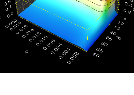
The behavior of the scalar field is determined by the damping term in (4), i. e. whether the initial conditions and the potential are chosen such that the field evolution is over-damped and the field is frozen to its initial value leading to a model nearly indistinguishable from a cosmological constant, or whether the damping plays only a minor role and the field evolves towards the potential minimum. (See Coble et al., (1997); Kawasaki et al., (2001) for a discussion in the case of the cosine potential.) Figure 1 displays the dependence of on the parameters and for the exponential potential (8) and the initial condition . Since we only discuss models with negative curvature, i. e. with , we show in figure 1 the parameter surface for only. Thus the plateau seen in figure 1 at corresponds to the cross section at , i. e. values of above this plateau correspond to solutions with positive curvature. Also shown are three curves corresponding to , respectively. The over-damped domain corresponds to small values of , i. e. to in order to give a significant value today. For the potentials (1) and (1) one obtains similar figures. The potential (9), however, does not display a sharp edge at which the evolution changes from frozen to rapidly evolving.
2 Potentials with a minimum


We now discuss the dependence of the angular power spectrum
of the CMB anisotropy
on the potentials (1) and (1).
The are compared with the 41 data points from
BOOMERanG (Netterfield et al.,, 2001),
MAXIMA-1 (Lee et al.,, 2001),
and DASI (Halverson et al.,, 2001).
The amplitude of the initial curvature perturbation is fitted
such that the value of is minimized with respect to
these three experiments,
where is computed using
RADPACK111See RADPACK homepage:
http://bubba.ucdavis.edu/~knox/radpack.html.
Figure 2 shows the dependence of on
the parameter for the hyperbolic-cosine potential (1)
with , i. e. .
The frozen case around , mimicking a cosmological constant,
gives a poorer fit than values around .
With increasing the fit deteriorates until a second
minimum is reached at .
The rapid dependence of on near
is due to the form of the solution curve of
in the - parameter space as shown by the inset.
Figure 3 shows the spectra for four different
models in comparison to the used experimental data.
The models belong to four different values of ,
i. e. , , ,
and , respectively.
These values were obtained for the initial condition
.
As explained in the Introduction, this choice does not represent
a restriction since another choice for would
be possible as well, but then other parameter values would be obtained
in order to leave at the assumed value.
This is in contrast to flat models where is
constraint to for all times by the
Friedmann equation.


The location of the first peak depends mainly on the sound horizon at last scattering and on the angular diameter distance to the surface of last scattering (SLS). For the models with the potential (1), shown in figure 3, the sound horizon is nearly the same because of . Since the angular diameter distance becomes smaller for larger values of , i. e. for a more dynamical field, the location of the peaks is shifted towards lower multipoles . This general trend is slightly modified by the oscillatory behavior of the field as is revealed by figure 3 where the first peak lies at , , and for , , and , respectively. Thus larger values of yield a first peak near even for . The position of the first peak for the model with is at a value of which is too high. For the models with larger the positions of the first peak are in agreement with the observations. The second and third peaks for the models with and occur at values of which are too low. The best description of the data is therefore given by the model with .
Although the two models with the largest -values seem to be similar with respect to their spectra, their magnitude-redshift relation is different as shown in figure 4. Here, the magnitude-redshift relation is compared with the data from Hamuy et al., (1996); Riess et al., (1998); Perlmutter et al., (1999) assuming an absolute magnitude of of supernovae Ia (Hamuy et al.,, 1996). The data is well described by the models with , and , but the curve belonging to gives values which are too low. Thus, the models with and are in agreement with the positions of the first acoustic peaks and the supernovae observations. The reason for this complementary behavior is revealed by figure 5, where the evolution of the equation of state as a function of conformal time is shown. The model with possesses a nearly frozen field, and thus increases only from to which cannot be seen in figure 5. The model with has whereas the remaining two models with and have already passed a phase with , in which the potential vanished and the kinetic term dominated. The supernovae measurements test the more recent history up to , which corresponds to for the latter two models. Therefore, the model with possesses a more negative effective averaged over from to . This in turn gives a better match with the supernovae observations.
The models have to provide an age of the universe compatible with the mean age of the oldest globular clusters of (Krauss,, 2001). The nearly frozen field case has an age of 13.0 Gyr, the model with has an age of 11.6 Gyr, whereas the model with has a low age of 9.9 Gyr because of its large mean value of . The case with leading to a lower mean value of gives 10.9 Gyr. In the last two cases the age may be too low if the error bounds in the age determination of globular clusters tighten. Altogether we see that the model with describes the CMB and supernovae data quite well and yields an age of the universe consistent with the oldest globular clusters.
Using the above initial conditions for the cosine potential (1) gives very similar results. The main difference is observed in the angular power spectrum for small values of . The increase in power for in figure 3 is due to an increased integrated Sachs-Wolfe contribution because of the gravitational instability of modes whose physical wavelength exceeds a critical value (Jeans wavelength) (Khlopov et al.,, 1985; Nambu and Sasaki,, 1990; Fabris and Martin,, 1997). That critical value can be obtained by expanding the potential at its minimum. The sign of the quartic term determines whether the gravitational instability is partially damped (positive sign as in (1)) or increased (negative sign as in (1)) relative to the purely quadratic potential (Khlopov et al.,, 1985). This leads to additional power for for the cosine potential (1) in comparison to the hyperbolic-cosine potential (1). This instability rules out potentials (1) and (1) with a parameter which leads to too much power at small values of . Such models are possible, however, in compact hyperbolic universes, such that the Jeans wavelength is larger than the largest wavelength of the eigenmode spectrum with respect to the Laplace-Beltrami operator. The largest wavelength belongs to the smallest eigenvalue of the compact fundamental cell. If the volume of the fundamental cell is small enough, the smallest eigenvalue would be sufficiently large, such that the largest wavelength would be smaller than the Jeans wavelength and no instability would occur. The effect of a finite size for nearly flat universes with respect to low multipoles is discussed in Aurich and Steiner, (2001) in connection with a special dark energy component having a constant .
3 Monotonic Potentials
Models with monotonically decreasing potentials begin with small values of the scalar field which then slides down the potential to ever increasing values of . The potentials with a minimum discussed above show that the location of the first acoustic peak depends on for fixed . Such behavior is also found in the case of the exponential potential (8). The inverse power potential (9), however, displays a nearly constant location of the first peak by specifying independent of in the range . E. g., for , i. e. , the first peak lies at . Thus the exponential potential is more flexible with respect to the peak position and, hence, does a better job in describing the observations. An example for , i. e. for , with is shown in figures 6 and 7, where the angular power spectrum and the magnitude-redshift relation is shown, respectively. These figures also show a model with where the quintessence contribution is increased to at the expense of the cold dark matter contribution which is lowered to . The first peak lies at for , and at for . The second and third acoustic peaks are also at the correct positions. Both models are compatible with the current CMB ( for and for ) and supernovae data. The low model provides the best match to the CMB data but it gives a power spectrum of the LSS which is too low as will be discussed in the next section. Both models give an age of 11.2 Gyr being at the low end of the allowed range. In these models has not yet reached its asymptotic value zero. In the recent past, which is tested by the supernovae data, had values of order . Figure 8 shows the dependence of on the parameter for , i. e. .


Another class of quintessence models specifies the equation of state instead of giving the potential. It is even possible to construct potentials which lead to a constant . The form of such potentials depends on the other energy components of the model. The simplest cases are a pure quintessence model, which leads to the exponential potential (8), and a radiation-dominated model, which gives the inverse power potential (9). With more components, analytic expressions of the potentials can be given only for special values of . For , the potential for a three-component model with radiation, matter and quintessence reads (Aurich and Steiner,, 2002)
| (10) |
with
and . The initial condition must be in order to enforce a constant also at the earliest times. This potential interpolates between the inverse power potential during the radiation epoch and the exponential potential during the quintessence epoch. The parameters , and are completely determined by the cosmological parameters at . The CMB angular power spectrum is shown in figure 9 for the two cases and , i. e. and , respectively. The first peak occurs at and , respectively. The model describes the data slightly better than the model with , and the second and third peaks also match better ( for and for ). The magnitude-redshift relation is nearly identical for both models, such that both curves cannot be separated in figure 10. The age of the universe is 11.7 Gyr in both cases.
Another potential can be derived for a two-component model consisting of matter and quintessence with (Aurich and Steiner,, 2002)
| (11) |
with
and . Here also the initial condition must be . Using this potential in a three-component model including radiation gives an equation of state which deviates from during the radiation epoch, but thereafter approaches very rapidly the limiting value . The corresponding models are shown in figures 11 and 12 for and , respectively. It is seen in figure 11 that the peaks in the CMB spectrum occur at values of which are larger than for the potential (10) ( for and for ). The magnitude-redshift relation is, however, in excellent agreement with the data as seen in figure 12. These models give with 12.5 Gyr and 12.4 Gyr older universes than the potential (10) with . Nevertheless, the model with describes the CMB data somewhat better than the model with .
4 The Large-Scale Structure
A further data set which the quintessence models have to explain is the power spectrum of the large-scale structure (LSS). In the following we compare the models with the power spectrum obtained from a compilation of galaxy cluster data by Peacock and Dodds, (1994) and with the decorrelated by Hamilton et al., (2000) using the IRAS Point Source Catalog Redshift Survey (PSC) (Saunders et al.,, 2000). These power spectra are shown in figures 13 to 15 as full squares (Peacock and Dodds,, 1994) and as circles (Hamilton et al.,, 2000). The linear regime is at wave numbers , where one expects a scale-independent bias parameter . For smaller scales, a scale-dependent bias is expected from -body simulations. A nearly flat CDM model (long dashed curve) is presented in figure 13 together with a CDM model without dark energy (dotted curve), where the latter has too much power at small scales. In addition figure 13 shows as solid curves the power spectra for the three quintessence models that agree with the CMB and supernovae data: the hyperbolic-cosine potential (1) with for (belonging to the highest lying of the three solid curves in figure 13), the exponential potential (8) with for , and the potential (10) for with the CMB normalization used in figures 3, 6 and 9, respectively. All three spectra show a very similar behavior and match the data obtained by Peacock and Dodds. Thus no bias factor is required for these models.


It is well known that quintessence models have less power than a CDM model where the dark energy is provided by the time-independent vacuum energy density. This is due to the suppression of growth of perturbations during the dark energy-dominated epoch. This epoch begins generally earlier in quintessence models than in CDM models (for a discussion of the flat case, see e. g. Coble et al., (1997); Wang and Steinhardt, (1998); Skordis and Albrecht, (2000); Doran et al., (2001)). To emphasize the point, figure 14 shows for the four hyperbolic-cosine quintessence models shown in figures 3 to 5. These models differ in the duration of the dark energy-dominated epoch. The long dashed curve in figure 14 belonging to shows the behavior for the frozen field, where increases from initially to only , i. e. this case is practically indistinguishable from a CDM model with a constant vacuum energy density. In this case the duration of the dark energy-dominated epoch is nearly the same as for a CDM model. Increasing from to , and thus enforcing a more dynamical field, reduces the duration of the matter-dominated epoch and, in turn, leads to lower LSS power as shown in figure 14.


The LSS power strongly depends on since the cold dark matter perturbations are not coupled to the radiation perturbations as is the case for the baryons before recombination. To stress that point, figure 13 shows also the results (short dashed curve) for the exponential potential (8) again for , where is decreased to and increased to . As shown in figure 7 this modification alters the magnitude-redshift relation only marginally. We would like to emphasize that the low model gives the best description of the CMB data (see figure 6) due to the enhanced amplitude of the first acoustic peak. The LSS power, however, requires then a bias factor of for as displayed by the short dashed curve in figure 13. The LSS dependence on is also demonstrated in figure 15, where the cold dark matter contribution is varied from to for the exponential potential (8) with . In comparison to CDM models, quintessence models need higher contributions of in order to compensate for the shorter matter-dominated epoch.
The LSS power is not only reduced by replacing the time-independent vacuum energy density by quintessence, but is additionally reduced by the negative curvature in comparison to flat models. The more negative the curvature, the more the LSS power is reduced (Wang and Steinhardt,, 1998). For the hyperbolic-cosine potential (1) in the nearly frozen case , the LSS power increases by a factor of 1.2 by increasing from 0.45 to 0.58 in models, i. e. by increasing from 0.85 to 0.98, despite the fact that the dark energy component is increased which by itself reduces the LSS power.

5 Conclusions
We have studied quintessence models with various potentials for a universe with negative curvature. We assumed thereby , and a scale-invariant Harrison-Zel’dovich spectrum. Several potentials have been found which are consistent with the current CMB anisotropy, supernovae and LSS data as well with the age of the universe with as small as . The best matches have been found for the hyperbolic-cosine potential (1), the exponential potential (8) and the potential (10) leading to a constant . In order to find agreement with the LSS data, it is necessary to use , which together with (for ) gives . Dynamical mass determinations lead to values in the range (Krauss,, 2001). Therefore our value belongs to the higher values of the allowed range. However, such a relatively large value is necessary in order to match the LSS observations. If future observations will favor higher values of , this would favor quintessence models in comparison to CDM models, because the latter have longer matter-dominated epochs and need therefore lower values of to achieve the same LSS power, since is fixed by BBN.
ACKNOWLEDGMENTS
We would like to thank the Scientific Supercomputer Centre (SSC) Karlsruhe for the access to their computers.
References
- Aurich and Steiner, (2001) Aurich, R. and Steiner, F. (2001). The cosmic microwave background for a nearly flat compact hyperbolic universe. MNRAS, 323:1016–1024.
- Aurich and Steiner, (2002) Aurich, R. and Steiner, F. (2002). Quintessence potentials with a constant equation of state. To be published elsewhere.
- Barreiro et al., (2000) Barreiro, T., Copeland, E. J., and Nunes, N. J. (2000). Quintessence arising from exponential potentials. Phys. Rev. D, 61:127301–1–4.
- Bean et al., (2001) Bean, R., Hansen, S. H., and Melchiorri, A. (2001). Early-universe constraints on dark energy. Phys. Rev. D, 64:103508–1–5.
- Becker et al., (2001) Becker, R. H., Fan, X., White, R. L., Strauss, M. A., Narayanan, V. K., Lupton, R. H., Gunn, J. E., Annis, J., Bahcall, N. A., Brinkmann, J., Connolly, A. J., Csabai, I., Czarapata, P. C., Doi, M., Heckman, T. M., Hennessy, G. S., Ivezic, Z., Knapp, G. R., Lamb, D. Q., McKay, T. A., Munn, J. A., Nash, T., Nichol, R., Pier, J. R., Richards, G. T., Schneider, D. P., Stoughton, C., Szalay, A. S., Thakar, A. R., and York, D. G. (2001). Evidence for reionization at : Detection of a Gunn-Peterson trough in a quasar. AJ, 122:2850–2857.
- Boughn and Crittenden, (2002) Boughn, S. P. and Crittenden, R. G. (2002). Cross-correlation of the cosmic microwave background with radio sources: Constraints on an accelerating universe. Phys. Rev. Lett. , 88:021302.
- Brax et al., (2000) Brax, P., Martin, J., and Riazuelo, A. (2000). Exhaustive study of cosmic microwave background anisotropies in quintessential scenarios. Phys. Rev. D, 62:103505–1–16.
- Caldwell et al., (1998) Caldwell, R. R., Dave, R., and Steinhardt, P. J. (1998). Cosmological imprint of an energy component with general equation of state. Phys. Rev. Lett. , 80:1582–1585.
- Chimento and Jakubi, (1996) Chimento, L. P. and Jakubi, A. S. (1996). Scalar field cosmologies with perfect fluid in Robertson-Walker metric. International Journal of Modern Physics D, 5:71–84.
- Coble et al., (1997) Coble, K., Dodelson, S., and Frieman, J. A. (1997). Dynamical models of structure formation. Phys. Rev. D, 55:1851–1859.
- Condon et al., (1998) Condon, J. J., Cotton, W. D., Greisen, E. W., Yin, Q. F., Perley, R. A., Taylor, G. B., and Broderick, J. J. (1998). The nrao vla sky survey. AJ, 115:1693–1716.
- Copeland et al., (1998) Copeland, E. J., Liddle, A. R., and Wands, D. (1998). Exponential potentials and cosmological scaling solutions. Phys. Rev. D, 57:4686–4690.
- Doran et al., (2001) Doran, M., Schwindt, J.-M., and Wetterich, C. (2001). Structure formation and the time dependence of quintessence. Phys. Rev. D, 64:123520–1–8.
- Fabris and Martin, (1997) Fabris, J. C. and Martin, J. (1997). Amplification of density perturbations in fluids with negative pressure. Phys. Rev. D, 55:5205–5207.
- Ferreira and Joyce, (1997) Ferreira, P. G. and Joyce, M. (1997). Structure formation with a self-tuning scalar field. Phys. Rev. Lett. , 79:4740–4743.
- Ferreira and Joyce, (1998) Ferreira, P. G. and Joyce, M. (1998). Cosmology with a primordial scaling field. Phys. Rev. D, 58:023503–1–23.
- Frieman et al., (1995) Frieman, J. A., Hill, C. T., Stebbins, A., and Waga, I. (1995). Cosmology with ultralight pseudo Nambu-Goldstone bosons. Phys. Rev. Lett. , 75:2077–2080.
- Halverson et al., (2001) Halverson, N. W., Leitch, E. M., Pryke, C., Kovac, J., Carlstrom, J. E., Holzapfel, W. L., Dragovan, M., Cartwright, J. K., Mason, B. S., Padin, S., Pearson, T. J., Shepherd, M. C., and Readhead, A. C. S. (2001). DASI first results: A measurement of the cosmic microwave background angular power spectrum. astro-ph/0104489.
- Hamilton et al., (2000) Hamilton, A. J. S., Tegmark, M., and Padmanabhan, N. (2000). Linear redshift distortions and power in the IRAS Point Source Catalog Redshift Survey. MNRAS, 317:L23–L27.
- Hamuy et al., (1996) Hamuy, M., Phillips, M. M., Suntzeff, N. B., Schommer, R. A., Maza, J., and Aviles, R. (1996). The absolute luminosities of the Calan/Tololo type IA supernovae. AJ, 112:2391–2397.
- Hu, (1998) Hu, W. (1998). Structure formation with generalized dark matter. ApJ, 506:485–494.
- Kawasaki et al., (2001) Kawasaki, M., Moroi, T., and Takahashi, T. (2001). Cosmic microwave background anisotropy with cosine-type quintessence. Phys. Rev. D, 64:083009–1–11.
- Khlopov et al., (1985) Khlopov, M. Y., Malomed, B. A., and Zeldovich, I. B. (1985). Gravitational instability of scalar fields and formation of primordial black holes. MNRAS, 215:575–589.
- Krauss, (2001) Krauss, L. M. (2001). Cosmology as seen from Venice. astro-ph/0106149. To appear in Conference proceedings, 9th International Workshop on Neutrino Telescopes, Venice, March 2001.
- Lee et al., (2001) Lee, A. T., Ade, P., Balbi, A., Bock, J., Borrill, J., Boscaleri, A., de Bernardis, P., Ferreira, P. G., Hanany, S., Hristov, V. V., Jaffe, A. H., Mauskopf, P. D., Netterfield, C. B., Pascale, E., Rabii, B., Richards, P. L., Smoot, G. F., Stompor, R., Winant, C. D., and Wu, J. H. P. (2001). A high spatial resolution analysis of the MAXIMA-1 cosmic microwave background anisotropy data. ApJL, 561:L1–L5.
- Ma and Bertschinger, (1995) Ma, C. and Bertschinger, E. (1995). Cosmological perturbation theory in the synchronous and conformal Newtonian gauges. ApJ, 455:7–25.
- Nambu and Sasaki, (1990) Nambu, Y. and Sasaki, M. (1990). Quantum treatment of cosmological axion perturbations. Phys. Rev. D, 42:3918–3924.
- Netterfield et al., (2001) Netterfield, C. B., Ade, P. A. R., Bock, J. J., Bond, J. R., Borrill, J., Boscaleri, A., Coble, K., Contaldi, C. R., Crill, B. P., de Bernardis, P., Farese, P., Ganga, K., Giacometti, M., Hivon, E., Hristov, V. V., Iacoangeli, A., Jaffe, A. H., Jones, W. C., Lange, A. E., Martinis, L., Masi, S., Mason, P., Mauskopf, P. D., Melchiorri, A., Montroy, T., Pascale, E., Piacentini, F., Pogosyan, D., Pongetti, F., Prunet, S., Romeo, G., Ruhl, J. E., and Scaramuzzi, F. (2001). A measurement by BOOMERanG of multiple peaks in the angular power spectrum of the cosmic microwave background. astro-ph/0104460.
- Peacock and Dodds, (1994) Peacock, J. A. and Dodds, S. J. (1994). Reconstructing the linear power spectrum of cosmological mass fluctuations. MNRAS, 267:1020–1034.
- Peebles and Ratra, (1988) Peebles, P. J. E. and Ratra, B. (1988). Cosmology with a time-variable cosmological ’constant’. ApJL, 325:L17–L20.
- Percival et al., (2001) Percival, W. J., Baugh, C. M., Bland-Hawthorn, J., Bridges, T., Cannon, R., Cole, S., Colless, M., Collins, C., Couch, W., Dalton, G., De Propris, R., Driver, S. P., Efstathiou, G., Ellis, R. S., Frenk, C. S., Glazebrook, K., Jackson, C., Lahav, O., Lewis, I., Lumsden, S., Maddox, S., Moody, S., Norberg, P., Peacock, J. A., Peterson, B. A., Sutherland, W., and Taylor, K. (2001). The 2dF Galaxy Redshift Survey: The power spectrum and the matter content of the universe. MNRAS, 327:1297–1306.
- Perlmutter et al., (1998) Perlmutter, S., Aldering, G., Della Valle, M., Deustua, S., Ellis, R. S., Fabbro, S., Fruchter, A., Goldhaber, G., Groom, D. E., Hook, I. M., Kim, A. G., Kim, M. Y., Knop, R. A., Lidman, C., McMahon, R. G., Nugent, P., Pain, R., Panagia, N., Pennypacker, C. R., Ruiz-Lapuente, P., Schaefer, B., and Walton, N. (1998). Discovery of a supernova explosion at half the age of the universe. Nature, 391:51–54.
- Perlmutter et al., (1999) Perlmutter, S., Aldering, G., Goldhaber, G., Knop, R. A., Nugent, P., Castro, P. G., Deustua, S., Fabbro, S., Goobar, A., Groom, D. E., Hook, I. M., Kim, A. G., Kim, M. Y., Lee, J. C., Nunes, N. J., Pain, R., Pennypacker, C. R., Quimby, R., Lidman, C., Ellis, R. S., Irwin, M., McMahon, R. G., Ruiz-Lapuente, P., Walton, N., Schaefer, B., Boyle, B. J., Filippenko, A. V., Matheson, T., Fruchter, A. S., Panagia, N., Newberg, H. J. M., Couch, W. J., and The Supernova Cosmology Project (1999). Measurements of Omega and Lambda from 42 high-redshift supernovae. ApJ, 517:565–586.
- Pryke et al., (2001) Pryke, C., Halverson, N. W., Leitch, E. M., Kovac, J., Carlstrom, J. E., Holzapfel, W. L., and Dragovan, M. (2001). Cosmological parameter extraction from the first season of observations with DASI. astro-ph/0104490.
- Ratra and Peebles, (1988) Ratra, B. and Peebles, P. J. E. (1988). Cosmological consequences of a rolling homogeneous scalar field. Phys. Rev. D, 37:3406–3427.
- Riess et al., (1998) Riess, A. G., Filippenko, A. V., Challis, P., Clocchiatti, A., Diercks, A., Garnavich, P. M., Gilliland, R. L., Hogan, C. J., Jha, S., Kirshner, R. P., Leibundgut, B., Phillips, M. M., Reiss, D., Schmidt, B. P., Schommer, R. A., Smith, R. C., Spyromilio, J., Stubbs, C., Suntzeff, N. B., and Tonry, J. (1998). Observational evidence from supernovae for an accelerating universe and a cosmological constant. AJ, 116:1009–1038.
- Sahni and Wang, (2000) Sahni, V. and Wang, L. (2000). New cosmological model of quintessence and dark matter. Phys. Rev. D, 62:103517–1–4.
- Sarbu et al., (2001) Sarbu, N., Rusin, D., and Ma, C. (2001). Strong gravitational lensing and dark energy. ApJL, 561:L147–L151.
- Saunders et al., (2000) Saunders, W., Sutherland, W. J., Maddox, S. J., Keeble, O., Oliver, S. J., Rowan-Robinson, M., McMahon, R. G., Efstathiou, G. P., Tadros, H., White, S. D. M., Frenk, C. S., Carramiñana, A., and Hawkins, M. R. S. (2000). The PSCz catalogue. MNRAS, 317:55–63.
- Seager et al., (1999) Seager, S., Sasselov, D. D., and Scott, D. (1999). A new calculation of the recombination epoch. ApJL, 523:L1–L5.
- Skordis and Albrecht, (2000) Skordis, C. and Albrecht, A. (2000). Planck-scale quintessence and the physics of structure formation. astro-ph/0012195.
- Steinhardt et al., (1999) Steinhardt, P. J., Wang, L., and Zlatev, I. (1999). Cosmological tracking solutions. Phys. Rev. D, 59:123504–1–13.
- Tytler et al., (2000) Tytler, D., O’Meara, J. M., Suzuki, N., and Lubin, D. (2000). Review of Big Bang nucleosynthesis and primordial abundances. Physica Scripta T, 85:12–31.
- Wang and Steinhardt, (1998) Wang, L. and Steinhardt, P. J. (1998). Cluster abundance constraints for cosmological models with a time-varying, spatially inhomogeneous energy component with negative pressure. ApJ, 508:483–490.
- (45) Wetterich, C. (1988a). Cosmologies with variable Newton’s ”constant”. Nuclear Physics B, 302:645–667.
- (46) Wetterich, C. (1988b). Cosmology and the fate of the dilatation symmetry. Nuclear Physics B, 302:668–696.
- Zlatev et al., (1999) Zlatev, I., Wang, L., and Steinhardt, P. J. (1999). Quintessence, cosmic coincidence, and the cosmological constant. Phys. Rev. Lett. , 82:896–899.