Hydrodynamic Interaction of Strong Shocks with Inhomogeneous Media - I: Adiabatic Case

Abstract

Many astrophysical flows occur in inhomogeneous (clumpy) media. We present results of a numerical study of steady, planar shocks interacting with a system of embedded cylindrical clouds. Our study uses a two-dimensional geometry. Our numerical code uses an adaptive mesh refinement allowing us to achieve sufficiently high resolution both at the largest and the smallest scales. We neglect any radiative losses, heat conduction, and gravitational forces. Detailed analysis of the simulations shows that interaction of embedded inhomogeneities with the shock/postshock wind depends primarily on the thickness of the cloud layer and arrangement of the clouds in the layer. The total cloud mass and the total number of individual clouds is not a significant factor. We define two classes of cloud distributions: thin and thick layers. We define the critical cloud separation along the direction of the flow and perpendicular to it distinguishing between the interacting and noninteracting regimes of cloud evolution. Finally we discuss mass-loading and mixing in such systems.

1 INTRODUCTION

Mass outflows play a critical role in many astrophysical systems ranging from stars to the most distant active galaxies. Virtually all studies of mass outflows to date have focused on flows in homogeneous media. However, the typical astrophysical medium is inhomogeneous with the ”clumps” or ”clouds” arising on a variety of scales. These inhomogeneities may arise due to initial fluctuations of the ambient mass distribution, the action of instabilities, variations in the flow source, etc. Whatever the origin of the clumps their effect can be dramatic. The presence of inhomogeneities can introduce not only quantitative but also qualitative changes to the overall dynamics of the flow.

A number of studies have attempted to understand the role of embedded inhomogeneities via (primarily) analytical methods (Hartquist et al., 1986), (Hartquist & Dyson, 1988), (Dyson & Hartquist, 1992), (Dyson & Hartquist, 1994). In these pioneering works it was suggested that interactions of the global flow with inhomogeneities may cause significant changes in the physical, dynamical, and even chemical state of the system. Two major consequences of the presence of clumps are mass-loading (i.e. seeding of material, ablated from the surface of inhomogeneities, into the global flow) and transition of the global flow into a transonic regime irrespective of the initial conditions. The papers cited above considered the potential effects of mass-loading on the global properties of a number objects in which inhomogeneities can be resolved. Such objects include planetary nebulae, e.g. NGC 2392 (O’Dell et al., 1990), (Phillips & Cuesta, 1999), and NGC 7293 (Burkert & O’Dell, 1998), and Wolf-Rayet stars, and primarily RCW58, which is believed to be mass-loading dominated (Hartquist et al., 1986).

A number of numerical studies of single clump interactions have been performed ((Klein et al., 1994) (hereafter KMC), (Anderson et al., 1994), (Jones et al., 1996), (Gregori et al., 1999), (Gregori et al., 2000), (Jun & Jones, 1999), (Miniati et al., 1999), (Lim & Raga, 1999)). In these papers the basic hydrodynamics or MHD of wind-clump and shock-clump physics have been detailed (often with microphysical processes included). A few studies of shock waves overrunning over multiple clumps exist in the literature (e.g. (Jun et al., 1996)). A detailed study of multiple clumps however, where an attempt is made to articulate basic physical processes and differentiate various parameter regimes, has not yet been carried out. In this paper, (and those which follow), we address the problem of clumpy flows providing a description of the dynamics of multiple dense clouds interacting with a strong, steady, planar shock.

The large parameter space and complexity of the problem require significant computational effort. To provide the necessary resolution of the flow we have used an adaptive mesh refinement method. This is a relatively new computational technology and because of this we have chosen to investigate so-called adiabatic flows in which radiative cooling is not considered. In this regard our approach is similar to that described by Klein et al. (1994) for single clumps and we will utilize their results in understanding our multi-clump simulations. We note that preliminary results, appropriate to AGN, were presented in (Poludnenko et al., 2001).

The plan of the paper is as follows. In Section 2 we describe the numerical experiments, the code used, and the formulation of the problem. In Section 3.1 we consider the general properties of the shock-cloud interaction in the context of the multi-cloud systems, primarily we focus on the four major phases of the interaction process. In Section 3.2 we discuss the role of cloud distribution in determining the dynamics of the system evolution. In Section 3.3 we define several key parameters, that allow us to distinguish between various regimes of shock-cloud interaction. Finally, in Section 3.4 we address the issue of mass-loading in such systems.

2 NUMERICAL EXPERIMENTS

2.1 Description of the Code Used

The code we used for this project is the AMRCLAW package which implements an adaptive mesh refinement algorithm for the equations of gas dynamics ((Berger & LeVeque, 1997), (Berger & Jameson, 1985), (Berger & Colella, 1989), (Berger & Oliger, 1984)). In the AMRCLAW approach, the computational domain is associated with a logically rectangular grid that represents the lowest level of refinement (level 1) and that embeds the nested sequence of logically rectangular meshes with finer resolution (levels 2,3,…). The temporal and spatial steps of all grids at a level L are refined with respect to the level L-1 grids by the same factor, typically 4 in our calculations. The mesh ratios $\Delta t/\Delta x$ and $\Delta t/\Delta y$ are then the same on all grids, ensuring stability with explicit difference schemes.

The core of the code - the AMR module - scans each refinement level every k time steps and regenerates all nested higher level grids in order to track the moving features of the flow. Two criteria are used to define cells requiring refinement: Richardson extrapolation and steepest gradient. The first criterion ensures that the local truncation error does not exceed some predefined tolerance. This is done via comparison of the solution obtained by taking 2 time steps on the existing grid with one computed by taking 1 time step on a grid that is twice as coarse in each direction. The second criterion ensures that the maximum of the gradients of all state variables does not exceed some predefined value and guarantees that sufficient refinement is achieved in such regions of the flow as shock waves, boundary layers, etc. Flagged cells are then organized into rectangular grid patches in a manner that provides a reasonable compromise between the size and the total number of individual patches. Finally, the AMR module of the code ensures that global conservation is preserved at grid interfaces via introduction of a conservative flux correction.

After the grid hierarchy is formed, each grid is forwarded to the integration module. This module considers every grid as an independent physical domain. The boundary conditions are obtained either from the physical boundary conditions of the computational domain or via interpolation from the neighbouring cells of the next lowest refinement level, depending on the grid location. This approach allows us to separate logically the AMR and integration modules, which facilitates incorporation of new features into the code. The integration proceeds by grid level starting at level 1, which is integrated over a time step, then at level 2 (it should be integrated over $R_{1}$=$x_{2}$/$x_{1}$= $y_{2}$/$y_{1}$=$t_{2}$/$t_{1}$ time steps to catch up), and so on. The solution on each grid is advanced via a second-order accurate Godunov-type finite volume method in which second-order accuracy is achieved via flux-limiting and proper consideration of transverse wave propagation. The multi-dimensional wave propagation algorithm is based on the traditional dimensional splitting with the Riemann problem solved in each dimension by means of a Roe-approximate Riemann solver (LeVeque, 1997). It should be noted, that our implementation of the Riemann solver, based on the Roe linearization, does not use any additional procedures to ensure satisfaction of the entropy condition, as usually employed for this type of Riemann solver. Our analysis shows that the numerical diffusion present in the system is sufficient to prevent entropy-violating waves from propagating in the system.

The hydrodynamic equations we solve are appropriate to a single-fluid system, although a passive tracer is introduced in order to track advection and mixing of the cloud material. This was implemented as an additional wave family in the Roe solver.

Our numerical experiments were performed on a coarse grid with the resolution of 50$\times$100 cells and with the maximum number of refinement levels equal to 3 (meaning that the coarse grid associated with the computational domain embeds not more than two nested higher resolution levels). Each higher level has a temporal and spatial step refined by the factor of 4 in comparison with the next lowest level and we kept this refinement ratio constant for all levels. Such setup provides the equivalent resolution of 800$\times$1600 cells. In order to facilitate comparison of our numerical experiments with those of KMC, we will describe the resolution not in terms of the equivalent resolution but in terms of the number of cells that fit in the original maximal cloud radius $a_{0}$, following the convention of KMC. Then all of the runs described here in our paper have 32 cells per cloud radius.

KMC suggested that a minimum resolution of 120 cells per cloud radius is necessary. We have performed the simulations of the cloud-shock interaction with the resolution of 120, 75, and 55 cells per cloud radius. Although we will not describe the details of those runs in this paper, the principal difference between the cases with maximum and minimum resolution, i.e. 120 and 32 cells per cloud radius, is the rate of instability formation at the boundary layers. This does not seem to have any significant effect on the global properties of the interaction or the averaged characteristics of the individual cloud ablation processes. Therefore, we find the resolution of 30 cells per cloud radius and above to represent accurately the global properties of the interaction process under consideration. Moreover, 30 cells per cloud radius is a reasonable compromise between maximizing the size of the computational domain and capturing as many small-scale features of the interaction process as possible.

Finally, another aspect of this problem is the connection between the spatial resolution (which naturally sets the smallest scale resolvable in the simulations) and the diffusion and thermal conduction length scales. As we will see in section 3.1.4, viscous diffusion and thermal conduction in a real physical system operate at length scales comparable to the size of a computational cell at the highest refinement level used in our simulations. Therefore, in a real system, features smaller than the ones that can be resolved with our resolution could not survive over the dynamical time scales relevant to the problem. We will address this in greater detail when we discuss the mixing phase of cloud evolution.

2.2 Formulation of the Problem

We set up a two-dimensional computational volume, associated with the initial condition of $N$ different clouds of radius $a_{i}$ and density $\rho_{i}$ embedded in the ambient medium of density $\rho_{a}$, and an incident shock wave. Since all of the experiments were performed in the Cartesian geometry, the clouds are actually cross-sections of the infinitely long cylinders. We will address the importance of the cloud shape in more detail in subsequent work where we will consider the fully 3-dimensional case of the shock interaction with spherical clouds. Denoting the maximum cloud radius present in the system as $a_{max}$, our computational domain is $25a_{max}\times 50a_{max}$. This allows us to track the dynamical evolution of the system over greater temporal and spatial intervals compared to the $6a_{max}\times 16a_{max}$ domain, considered by KMC.

All our calculations were performed in a fixed reference frame in which both the clouds and the ambient medium are stationary at time $t=0$. In this reference frame the horizontal axis is taken to be the x axis, the vertical axis - y axis. Initially both the clouds and the surrounding intercloud medium are assumed to be in pressure equilibrium and have pressure $P_{0}$. Typically, the extent of the region, occupied by the cloud distribution at time $t=0$, is taken to be not more than 30-35$\%$ of the horizontal extent of the computational domain with $X_{L}$ offset by 5$\%$ from the left boundary of the computational domain and $X_{R}$ offset by 35-40$\%$. Table 1 below, describing the numerical experiments discussed in this paper, provides the details of the cloud distribution in each simulation. Figure 1 illustrates the setup of the computational domain at $t=0$.

In the most general case we assume each cloud to have the same nonuniform density profile. The clouds have constant density up to a smoothing transition region at the cloud edge which is achieved through a linear or $\tanh(r)$ function. We typically set the extent of the transition region to the outer $20\%$ of a cloud radius $a_{i}$ and use the $\tanh(r)$ - type smoothing function. Therefore, the cloud density profile is of the form

$$\rho_{i}(r)=\left\{\begin{array}[]{ll}\rho_{i}=Const,&0\leq r\leq r_{i}\\ \displaystyle\frac{\rho_{a}+\rho_{i}}{2}+\frac{\rho_{a}-\rho_{i}}{2}\ \cdot\ \frac{\tanh\big{(}r-\frac{a_{i}+r_{i}}{2}\big{)}}{\tanh\big{(}\frac{a_{i}-r_{i}}{2}\big{)}},&\ r_{i}\leq r\leq a_{i}\end{array}\right.$$ (1)

Although there is very little observational data available concerning the internal structure of embedded clouds this particular choice of the density profile seems to be a sufficiently good approximation to the real physical clouds and inhomogeneities. Burkert and O’Dell (Burkert & O’Dell, 1998) discussed the evidence for the exponential density profile in the cometary knots of NGC 7293 (Helix nebula) which is similar to the density profile used by us.

In the simple adiabatic interaction of a cloud with a shock wave there are two dimensionless parameters that completely define the problem: Mach number of the blast wave, $M_{S}$, and the density contrast between the cloud and the intercloud medium

$$\chi_{i}\equiv\frac{\rho_{i}}{\rho_{a}}.$$ (2)

The range of values spanned by the density contrast $\chi$ can be quite large and is the most important parameter of the problem. For the astrophysical situations of interest this range can often cover up to 5 orders of magnitude (from 10 to $10^{6}$), presenting a significant challenge both for the numerical modeling and for the subsequent interpretation and analysis of the results. In order to decrease the extent of this dimension of the parameter space, we chose a “compromise” value of the parameter $\chi$ to be 500. Although the runs we discuss in this paper all use this value of the density contrast, we will briefly discuss numerical experiments with $10\lesssim\chi\lesssim 1000$ in the results section, particularly in the context of the problem of mass loading. We will provide a more comprehensive study of scaling with density contrast in the subsequent work.

Another important parameter is the shock wave Mach number $M_{S}$. We consider a planar steady shock wave propagating into the computational domain from the left. Since we operate in the reference frame in which both the clouds and the ambient medium are stationary, the shock wave Mach number completely defines the shock velocity as well as the conditions of the postshock flow. Using the sound speed of the ambient medium $C_{a}=(\gamma{P_{0}}/\rho_{a})^{1/2}$, the shock velocity in the stationary reference frame takes the form

$$v_{S}=M_{S}\Big{(}\frac{\gamma{P_{0}}}{\rho_{a}}\Big{)}^{\frac{1}{2}}.$$ (3)

Using the Rankine-Hugoniot relations (Landau & Lifshitz, 1959) we have the following expressions for the postshock conditions

$$\rho_{PS}=\rho_{a}\bigg{(}1-\frac{2}{\gamma+1}\Big{(}1-\frac{1}{M_{S}^{2}}\Big{)}\bigg{)}^{-1},$$ (4)

$$P_{PS}=\displaystyle P_{0}\bigg{(}1+\frac{2\gamma}{\gamma+1}\Big{(}M_{S}^{2}-1\Big{)}\bigg{)}=\displaystyle\frac{2}{\gamma+1}\rho_{a}v_{S}^{2}\bigg{(}1-\frac{\gamma-1}{2\gamma M_{S}^{2}}\bigg{)},$$ (5)

$$v_{PS}=\frac{2v_{S}}{\gamma+1}\Big{(}1-\frac{1}{M_{S}^{2}}\Big{)}.$$ (6)

We assume that the shock wave is strong, so that the condition

$$\Pi=\bigg{(}\frac{P_{PS}-P_{0}}{\rho_{a}C_{a}^{2}}\bigg{)}\gg 1$$ (7)

is satisfied.

Shock wave Mach numbers in astrophysical situations can cover a large range of values. Fortunately, the problem becomes practically independent on the Mach number for strong shocks, i.e. for $M_{S}\approx 10$ and above. Indeed, as it can be seen from the shock conditions (4) - (6), for $M_{S}\lesssim 10$ the postshock density $\rho_{PS}$, pressure $P_{PS}$, and velocity $v_{PS}$ are at most within a few percent of their respective values at $M_{S}\rightarrow\infty$. Moreover, recalling that there is scale invariance inherent in the hydrodynamic equations under transformations

$$t\rightarrow tM_{S},\quad v\rightarrow v/M_{S},\quad P\rightarrow P/M_{S}^{2},$$ (8)

the conclusion follows that for $M_{S}\gg 1$ the time evolution of a cloud does not depend on the Mach number of the shock (Klein et al., 1994). Indeed, the results of KMC show that for the difference in $M_{S}$ of 2 orders of magnitude ($10-1000$) time evolution of the system does not differ by more than 15$\%$. We will see that our results fully corroborate the presence of Mach scaling in the problem under consideration.

We assume that the structure of the postshock flow does not change in time for the duration of the simulations. An example of such steady postshock flow is the wind from a post-AGB star driving a shock with a constant postshock flow structure into a slow wind ejected during the previous stages of evolution. This frees us from having to use the pressure variation timescale $t_{P}$ to constrain a cloud size, since we can set $t_{P}\rightarrow\infty$. On the other hand, for blast waves one cannot assume a steady time independent postshock flow (for example, SNR blast waves) and the size of the clouds is constrained by the condition $t_{CC}\ll t_{P}$ as discussed by KMC (see (Klein et al., 1994)).

It should be mentioned that the maximum cloud size is still constrained by the condition of the shock front planarity. This condition is less restrictive than the one discussed above, however it still requires a cloud diameter not to exceed $5-10\%$ of the global shock wave front radius. This condition is satisfied, for example, in the case of the inhomogeneities, or the cometary knots, observed in such planetary nebulae as NGC 2392 and NGC 7293 (e.g. (Burkert & O’Dell, 1998)).

The timescale we use to define time intervals in our numerical experiments is the time required for the incident shock wave to sweep across an individual cloud, called the shock-crossing time,

$$t_{SC}=\frac{2a_{max}}{v_{S}},$$ (9)

where $a_{max}=a_{0}$ for cloud distributions with identical clouds and $a_{max}=max(a_{i})$ for cloud distributions of varying size clouds.

Due to the scale-invariance of our simulations, one can, using specific values for the shock velocity and the size of the inhomogeneities, easily convert the time units used in our discussion into the physical ones. $t_{SC}$ is particularly useful to characterize the problem since it has clear physical meaning and does not depend on a specific density contrast, which is important in the case of systems containing clouds of different density.

Note that except for the very short period of time when a cloud interacts with the shock front, the former finds itself immersed in a post-shock flow or “wind” the pressure and density of which vary only by several percent over the large range of Mach numbers. Since KMC showed that the initial interaction with the shock front does not alter the evolution of the system for the varying Mach number, the details of the evolution should not change after the shock front passed the cloud. Therefore, conclusions about Mach scaling should be valid both for the durations of cloud-wind interactions discussed by KMC, and for the much longer durations in our experiments.

One final remark should be made concerning the boundary conditions used in our experiments. In all runs we imposed a constant inflow at the left boundary, described by the postshock conditions, which is determined using the relations (4)-(6), and open boundary conditions at the right, top, and bottom boundaries. Those outflow boundary conditions were implemented via 0-order extrapolation.

2.3 Description of the Runs

All of the runs discussed in this paper contain a Mach 10 shock wave as a part of the initial conditions and embedded clouds with the density contrast of 500. Table 1 presents a summary of our numerical experiments.

In addition to the dependence on the shock Mach number and the cloud density contrast there are other degrees of freedom present even in the simplest adiabatic case. We considered how the dynamical evolution, e.g. rate of momentum transfer from the shock wave and shock deceleration, mass loading, mixing of cloud material, etc. of the system depend on

$\bullet$ the number of clouds present in the system;

$\bullet$ total cloud mass;

$\bullet$ spatial arrangement of clouds;

$\bullet$ individual cloud sizes and masses.

In most of the runs we constrained ourselves to the case of identical clouds, varying only their number and arrangement. Radii of the clouds in all runs except $M14_{r}$ is 2$\%$ of the horizontal extent of the computational domain. In order to simplify consideration of the dependence on a specific cloud arrangement, most runs have a regular cloud distribution, where the clouds are placed in the vertices of the mesh, formed by the centers of the clouds in the run M14. In addition, we considered a more general case of a random cloud distribution with random cloud spatial positions and radii.

All of our numerical experiments were run for about 100 $t_{SC}$ . By this time each individual cloud has almost completely lost its identity and gained a velocity comparable to the velocity of the global flow. Mixing of cloud material with the global ambient flow is nearly completed by 100 $t_{SC}$ as well.

In order to facilitate our analysis, we track temporal evolution of the global averages and one-dimensional spatial distributions of several quantities, namely

$\bullet$ kinetic energy fraction, $\eta_{kin}=E_{kin}/E_{tot},$

$\bullet$ thermal energy fraction, $\eta_{term}=E_{term}/E_{tot},$

$\bullet$ volume filling factor $\nu.$

In order to obtain those quantities from the complex data structure of the adaptive mesh simulations, we project the values of the state vector from each grid of the AMR grid hierarchy onto a uniform grid with the resolution of the highest refinement level and that is associated with the computational domain. Such projection does not cause loss of data or its precision. When this projection is done, we define the global averages of the first two quantities above as

$$\langle\xi\rangle_{2D}=\frac{\displaystyle\sum_{i=1}^{N_{i}}\sum_{j=1}^{N_{j}}\xi_{ij}}{N_{i}N_{j}}\approx\frac{\displaystyle\int_{x_{min}}^{x_{max}}\int_{y_{min}}^{y_{max}}\xi(x,y)dxdy}{(x_{max}-x_{min})(y_{max}-y_{min})},$$ (10)

where $\xi$ stands for the quantity being considered, and $N_{i}$, $N_{j}$ are the numbers of cells of the projected grid in the $x$ and $y$ direction correspondingly. Such averaging allows us to follow momentum transfer from the shock wave to the system of clouds, in the case of $\langle\eta_{kin}\rangle_{2D}$, and heating of the cloud system and intercloud material, in the case of $\langle\eta_{term}\rangle_{2D}$.

We also define the one-dimensional spatial averages of those two quantities as

$$\langle\xi\rangle_{1D}(x)=\frac{\displaystyle\sum_{j=1}^{N_{j}}\xi_{ij}}{N_{j}}\approx\frac{\displaystyle\int_{y_{min}}^{y_{max}}\xi(x,y)dy}{(y_{max}-y_{min})},$$ (11)

where $\xi$ again stands for the quantity under consideration.

Our code follows advection of a passive tracer marking cloud material. In order to follow mixing of the cloud material with the global flow, we define the global average of the volume filling factor $\langle\nu\rangle_{2D}$ as the ratio of the total number of cells containing cloud material to the total number of cells in the computational domain. We also define the one-dimensional spatially averaged volume filling factor $\langle\nu\rangle_{1D}$ as the variation with the coordinate $x$ of the ratio of the number of cells containing cloud material in each vertical row of the computational grid to the total number of cells in the vertical dimension.

3 RESULTS

3.1 General Properties of the Shock-Cloud Interaction

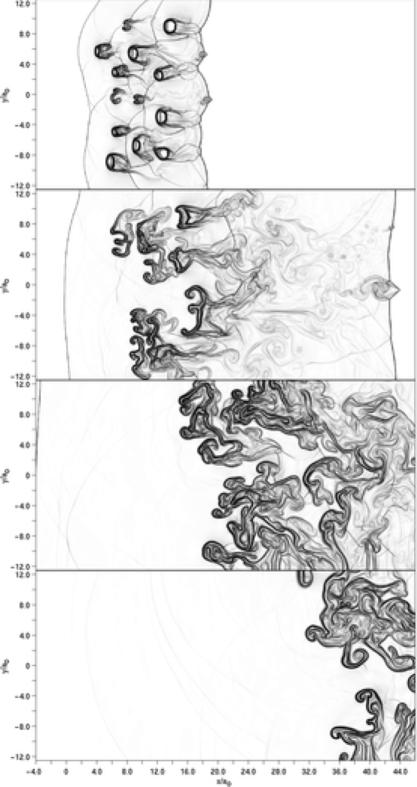
Figure 5: Run $M14_{r}$. Time evolution of a system, containing fourteen clouds in a random distribution and interacting with a $M_{S}=10$ shock wave. Shown are the synthetic Schlieren images of the system at times $9.71\ t_{SC}$, $22.47\ t_{SC}$, $45.43\ t_{SC}$, $69.09\ t_{SC}$.

Figures 2 - 5 show the time evolution of a shock wave interacting with a single cloud (run $M1$), three clouds (run $M3$), fourteen identical clouds in the regular distribution (run $M14$), and fourteen clouds of random size in a random distribution (run $M14_{r}$). Shown are the synthetic Schlieren images of the system at four different times for all four sequences. Each image is obtained by calculating the density gradient at each point, plotted on a gray scale with the white denoting zero and black - the maximum density gradient. Every image in each sequence roughly illustrates transitions between the evolutionary phases discussed below.

3.1.1 Initial Compression Phase

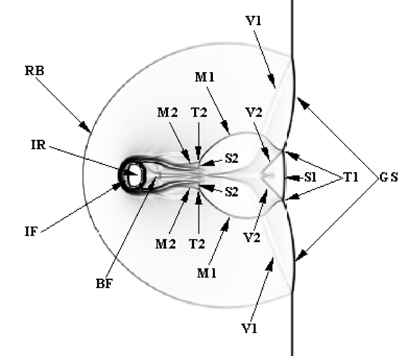
Figure 6: Flow structure during the initial compression phase. Shown is the Schlieren image of the run $M1$ at time $5.1\ t_{SC}$. $GS$ - external global forward shock; $RB$ - external reverse bow shock; $IF$ - internal forward shock; $IR$ - internal reverse shock; $BF$ - back flow, caused by global forward shock convergence on the symmetry axis; $V1$ - primary vortex sheets, caused by regular reflection of the bow shock; $M1$ - primary Mach reflected shocks, caused by Mach reflection of the global forward shock at the symmetry axis; $S1$ - primary Mach stem (more precisely, two primary Mach stems); $T1$ - primary triple points; $V2$ - secondary vortex sheets, caused by the primary Mach reflection of the global forward shock (note the two stem bulges formed at the base of the secondary vortex sheets near the symmetry axis); $M2$ - secondary Mach reflected shocks; $S2$ - secondary Mach stems; $T2$ - secondary triple points.

After initial contact, an external shock transmits an internal forward shock into a cloud. This causes cloud compression and heating. At the same time a bow shock forms around the cloud. KMC subdivide this phase into two stages: initial transient and shock compression. Our numerical experiments show that, in general, their description is applicable for all cloud distributions except for the cases when individual clouds are almost in contact at time $t=0$. However, we do not typically see a reverse shock propagating inside the cloud as they did at later stages. The cloud interior seems to be dominated by the forward shock wave which prevents a reverse shock from detaching from the back surface of the cloud. The absence of the reverse shock is the reason for lower maximum densities in the cloud interior during this compression phase compared with KMC: we typically see $\rho_{i,max}\lesssim 3\rho_{i,0}$ as opposed to $\rho_{i,max}\lesssim 10\rho_{i,0}$, quoted by KMC. Figure 6 illustrates the major flow structures present in the system during the initial compression phase.

Propagation of the forward shock in the cloud allows us to define another important time scale governing the evolution of the system and defining the duration of the compression phase: the cloud crushing time $t_{CC}$ . This is the time necessary for the internal forward shock to cross the cloud and reach its downstream surface

$$t_{CC}=\frac{2a_{max}}{v_{CS}}.$$ (12)

In the above expression $v_{CS}$ is the internal forward shock velocity and $a_{max}$ is again defined as $a_{0}$ in the cases of cloud distributions with identical clouds, and as $max(a_{i})$ in the cases of cloud distributions with clouds of varying size. Following KMC, the velocity of the internal forward shock can be written as

$$v_{CS}\simeq\frac{v_{S}}{\chi^{1/2}}\Bigg{(}\frac{\gamma+1}{8/3}\Bigg{)}^{1/2}\big{(}F_{c1}F_{st}\big{)}^{1/2},$$ (13)

where $v_{S}$ is the velocity of the external shock. The factor $F_{st}$ relates the external postshock pressure far upstream with the stagnation pressure at the cloud stagnation point and has the form (Klein et al., 1994)

$$F_{st}\simeq 1+\frac{2.16}{1+10.7\{(\gamma+1)\chi\}^{-1/2}}.$$ (14)

The factor $F_{c1}$ relates the stagnation pressure with the pressure just behind the internal forward shock and has an approximate value of 1.3 determined from numerical experiments (Klein et al., 1994).

While we will primarily use the shock-crossing time as the major time scale, we will occasionally give time in terms of the cloud crushing time to facilitate comparison with the results discussed by KMC. For this purpose we express the cloud crushing time in terms of the shock crossing time. Recalling the definition of $t_{SC}$ (9) we have

$$t_{CC}=\Bigg{(}\chi^{1/2}\Big{(}\frac{8/3}{\gamma+1}\Big{)}^{1/2}\big{(}F_{c1}F_{st}\big{)}^{-1/2}\Bigg{)}t_{SC}.$$ (15)

Therefore, for the case of $\chi=500$

$$t_{CC}=12\ t_{SC},$$ (16)

which agrees to about a few percent with the results of the numerical experiments.

The global properties of the flow at this stage are characterized by the onset of individual bow shocks around each cloud in a time of order $t_{SC}$. By the end of the initial compression phase those individual bow shocks merge into a single bow shock.

Finally, the downstream flow, i.e. the flow right behind the external forward shock front, is effected by the onset of turbulence in the tails behind the clouds.

3.1.2 Re-expansion Phase

This phase is initiated after the cloud internal forward shock reaches the back of the cloud. The two major processes then occur: lateral expansion of the cloud and the onset of instabilities at its upstream surface. At this stage Rayleigh-Taylor type instabilities dominate at the cloud/ambient flow interface. These are driven in part by the cloud expansion and incipient large-scale fragmentation. The flow downstream with respect to the clouds is dominated by Kelvin-Helmholtz instabilities operating in the growing turbulent region. The combined action of the lateral expansion and the instabilities causes the clouds to take the “umbrella-type” shape and eventually break up.

In the context of those two processes, the initial cloud separation becomes of key importance defining the subsequent behaviour of the whole system. We will see below that it can be used to distinguish between the two regimes of cloud evolution: interacting and noninteracting, and can serve as the basis for classification of cloud distributions. In subsection 3.3 we will give more rigorous discussion of the role of cloud separation. For now we give a qualitative illustration.

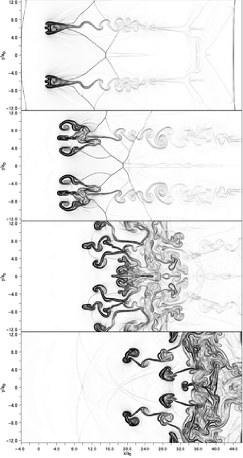
Figure 7: Run $A2$. Illustration of the non-interacting regime of cloud evolution: interaction of a $M_{S}=10$ shock wave with a system of two identical clouds with the cloud center separation of $12.0\ a_{0}\approx 2.86\ d_{crit}$. Shown are the synthetic Schlieren images of the system at times $22.47\ t_{SC}$, $35.23\ t_{SC}$, $50.54\ t_{SC}$, $68.40\ t_{SC}$.

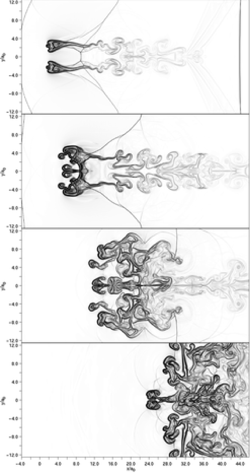
Figure 8: Run $M2$. Illustration of the interacting regime of cloud evolution: interaction of a $M_{S}=10$ shock wave with a system of two identical clouds with the cloud center separation of $4.0\ a_{0}\approx 0.95\ d_{crit}$. Shown are the synthetic Schlieren images of the system at times $22.47\ t_{SC}$, $35.23\ t_{SC}$, $50.54\ t_{SC}$, $68.40\ t_{SC}$.

Clouds, located far enough from each other, are not greatly influenced by their neighbours and their interaction with the flow proceeds independently as described by KMC. This case is illustrated in Figure 7. Compared to the evolution of a single cloud system, shown in Figure 2, the two clouds evolve up to the point of their destruction very similarly to the single cloud case. However, cloud separations can be small enough for the mutual interaction to manifest early during the re-expansion phase, as in Figure 8. This mutual interaction causes changes primarily in the flow between clouds. As a result the lateral expansion and growth of the Rayleigh-Taylor instabilities in the cloud material is affected. The tails behind the clouds are also deformed outwards (see, for example, as well Figure 3).

The unperturbed supersonic flow that forms behind the external shock wave undergoes a transition from a supersonic to a subsonic regime as it passes through a cloud bow shock. As a consequence it suffers a significant velocity drop whose magnitude is larger for smaller cloud separations due to the larger volume of the stagnation zone in front of the clouds. Clouds, acting as the Lavalle nozzles, then cause the flow material to re-accelerate. The flow reaches a sonic point next to a cloud core for the regions of the flow adjacent to a cloud, and further downstream for the regions of the flow located further from the clouds. It is important to note that this re-acceleration results in rarefaction of the flow and a gradual decrease both of thermodynamic and dynamical pressure. Eventually, as a result of acceleration in the intercloud region, the flow becomes highly supersonic and finally shocks down through a stationary shock formed downstream of the clouds to the regime close to the unperturbed flow behind the external shock (see Figures 7-8).

From the above discussion it is clear that the lateral expansion velocity depends critically on the cloud separation. For sufficiently low flow speeds the cloud material will expand at the cloud internal sound speed. With increasing global flow velocities (or, equivalently, with increasing velocities of the external shock front) the lateral expansion velocity will increase as well. This velocity is limited, in principle, by the terminal expansion velocity into vacuum.

For a fixed unperturbed upstream flow, the flow velocity near a cloud lateral surface (facing the space in between the clouds) will be the highest in the case of a single cloud or a cloud located far from the neighbouring ones. With decreasing cloud separation this velocity will decrease as well, causing higher dynamical pressure on the lateral surface and, therefore, lower lateral expansion velocities. This occurs because the velocity drop across a bow shock in the cases of small cloud separations is much larger due to a stronger stagnation effect in between the bow shock and the clouds. Therefore, flow adjacent to the cloud does not reach velocities as high as in cases of large cloud separations . Another way to look at this process is the following. The flow adjacent to the cloud surface passes through a sonic point but, in the cases of small cloud separations, densities in the stagnation region are much higher. Thus flow densities at the sonic point near the cloud lateral surface are much higher. This leads to lower sound speeds and, therefore, lower flow speeds.

Following KMC, the effective lateral expansion velocity $v_{exp}$ can be defined as the internal cloud sound speed

$$v_{exp}=C_{C}=v_{CS}\frac{\big{(}2\gamma(\gamma-1)\big{)}^{\frac{1}{2}}}{\gamma+1},$$ (17)

where $v_{CS}$ is the velocity of the cloud internal forward shock (13). Our numerical experiments prove this to be a very good approximation during almost all of the re-expansion phase. The expansion velocity exceeds this value by the end of the re-expansion phase due to stagnation pressure in the regions, formed by the Rayleigh-Taylor instability.

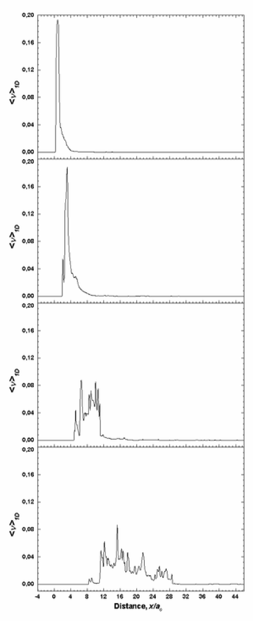
Figure 12: Distribution of cloud material along the horizontal dimension of the computational domain for the run $M3$. Shown are the one-dimensional spatial averages of the volume filling factor $\langle\nu\rangle_{1D}$ at times $12.26\ t_{SC}$, $25.02\ t_{SC}$, $37.78\ t_{SC}$, $50.54\ t_{SC}$.

We are now in a position to articulate the temporal evolution of a cloud radius in the direction perpendicular to the upstream flow. From the moment of their initial contact with the external shock to the moment of their destruction, the clouds first undergo slight compression in the direction perpendicular to the flow and subsequently re-expand. KMC’s analytic model did not explicitly include cloud compression but instead tried to account for its effect via a reduced monotonic expansion rate from $t=0$. Since $a_{\perp}(t)$ is intimately related to the drag exerted on a cloud by the global flow, the theoretical rate of the momentum pickup by a cloud (or the rate of cloud deceleration in the reference frame used by KMC) differed from the numerical result. Namely, in Figure 12b of the paper by KMC numerical and theoretical results are practically the same up to the time $\approx 2.0t_{CC}$, when the rate of cloud deceleration suddenly increases and the numerical and theoretical results drastically diverge. This moment of time corresponds to the beginning of the re-expansion phase, when the cloud cross-section starts to increase causing an increase of the rate of the momentum transfer from the flow to the cloud. To avoid this problem and simplify an expression for $a_{\perp}(t)$ we use the following form for evolution of a cloud radius normal to the flow,

$$a_{\perp}(t)=\left\{\begin{array}[]{ll}a_{0},&t\leq t_{CC}\\ a_{0}+C_{C}(t-t_{CC}),&t_{CC}\leq t\leq t_{CD}.\end{array}\right.$$ (18)

Here, $C_{C}$ is given by (17), and $t_{CD}$ is the cloud destruction time, defined below in (19).

3.1.3 Cloud Destruction Phase

Depending on the cloud separation, via the process of re-expansion clouds may come into contact and merge into a single coherent structure. This subsequently interacts with the flow as a whole and eventually breaks up. Thus for the case of small cloud separations we can define the moment of cloud merging as the onset of the cloud destruction phase. For large cloud separations in which individual clouds get destroyed before ever merging, it is difficult to define the precise onset of the destruction phase as it may be effectively viewed as a part of the re-expansion phase.

We define the end of the cloud destruction phase as the time when the largest cloud fragment contains less than 50$\%$ of the initial cloud mass. For single cloud systems or systems of weakly interacting clouds we define the total time from $t=0$ until the end of the cloud destruction phase as the cloud destruction time $t_{CD}$,

$$t_{CD}=\alpha t_{CC}=\alpha^{\prime}t_{SC}.$$ (19)

Typically $\alpha\approx 2.0$ consistent with KMC, and using (16) we find $\alpha^{\prime}\approx 24$ in our simulations.

In addition to $t_{CD}$ there is also a cloud system destruction time $t_{SD}$ which we define as the time when the largest fragment of a cloud located furthest downstream contains less than 50$\%$ of its initial mass. For thick layer systems (to be described later), including strongly interacting cloud distributions, $t_{CD}$ becomes less relevant as a description of the system than $t_{SD}$ because $t_{CD}\ <\ t_{SD}$.

3.1.4 Mixing Phase

After the end of the destruction phase cloud material velocity is still only a small fraction of the global flow velocity (see (42) below). The velocity difference promotes Kelvin-Helmholtz instabilities at the cloud material - global flow interfaces and, therefore, the transition of the system to a turbulent regime. Typically by the beginning of this phase each cloud has lost its identity as a result of merging with neighbouring clouds. As the individual fragments become smaller and the velocity of the global flow relative to the cloud material decreases, Kelvin-Helmholtz instabilities grow faster than the Rayleigh-Taylor type ones. This eventually results in complete domination by the former of the small-scale fragmentation and causes mixing of cloud material with the flow (Klein et al., 1994).

In our numerical experiments, as it can be seen in Figures 2 - 5, turbulent mixing produces a two-phase filamentary system. The appearance of such a two-phase system results because our code does not include viscous diffusion or thermal conduction restricting all dissipative effects to numerical diffusion only. The latter acts at the length scales comparable with a cell size at the highest refinement level.

Real dissipative effects also constrain the overall stability of cold dense plasma embedded in a tenuous hotter medium. KMC considered the overall effect of thermal conduction on the stability of such two-phase media against evaporation. They concluded that the cloud ablation time due to evaporation, expressed in terms of the shock-crossing time $t_{SC}$, defined in (9) above, has the form

$$t_{ab}=\frac{\chi}{9F(\sigma^{\prime}_{0})}\Bigg{(}\frac{2}{\gamma+1}\Bigg{)}^{\frac{1}{2}}\Big{(}F_{c1}F_{st}\Big{)}^{-\frac{1}{2}}t_{SC},$$ (20)

where $F(\sigma^{\prime}_{0})$ is typically of order unity (Klein et al., 1994). Therefore, for the case of our simulations, the typical ablation time is $t_{ab}\sim 30t_{SC}$, or comparable to the cloud destruction time.

One can also estimate an effective depth over which diffusion and thermal conduction will disrupt the boundary layer between the two phases over a dynamical time-scale, $t_{SC}$. This can be estimated as follows (see (Kuncic et al., 1996) and references therein). For viscous diffusion

$$d_{diff}\sim(D_{diff}t_{SC})^{\frac{1}{2}}=\Bigg{(}\bigg{(}\frac{2}{\gamma}\bigg{)}^{\frac{1}{2}}\frac{1}{M_{S}n_{0}\sigma}a_{0}\Bigg{)}^{\frac{1}{2}},$$ (21)

where $D_{diff}$ is the diffusion coefficient and $n_{0}$ is the initial cloud number density. If we assume $n_{0}\sim 1000\ cm^{-3}$ then, for the cases presented in our simulations, $d_{diff}$ is about $1\%$ of the initial cloud radius, or equivalently is about $1/5$ of a cell of the computational domain at the highest refinement level. For thermal conduction, the effective depth is

$$d_{term}\sim(D_{term}t_{SC})^{\frac{1}{2}}=\Bigg{(}\bigg{(}\frac{2}{\gamma}\bigg{)}^{\frac{1}{2}}\frac{1}{M_{S}n_{0}\sigma_{p}}\bigg{(}\frac{m_{p}}{m_{e}}\bigg{)}^{\frac{1}{2}}a_{0}\Bigg{)}^{\frac{1}{2}}=d_{diff}\bigg{(}\frac{m_{p}}{m_{e}}\bigg{)}^{\frac{1}{4}}.$$ (22)

Then $d_{term}$ is about $6\%$ of $a_{0}$, or equivalently, about twice the size of a computational cell at the highest refinement level. Therefore, should we have included real dissipative effects they would destroy the smallest resolvable structures over the dynamically relevant time scales. Consequently, any further increase in resolution without providing for the appropriate mechanisms, capable to inhibit significantly diffusion and thermal conduction, would not provide additional insights into the real physical evolution of a system.

The importance of the dissipative effects is two-fold. First consider the stability of the initial system against destruction due to thermal conduction and diffusion. From the arguments given above dissipative effects prevent survival of the system for any dynamically significant amount of time. As a solution to this problem, KMC suggested that weak magnetic fields inhibit thermal conduction and diffusion. Indeed, as it was shown by (Mac Low et al., 1994), evolution of weakly magnetized clouds during the compression and re-expansion phases does not differ significantly from the purely hydrodynamic description. However the presence of magnetic fields would raise other issues. During the mixing phase the system undergoes transition to turbulence which may amplify the initially dynamically insignificant magnetic fields. Turbulence can lower values of the plasma parameter $\beta=P_{g}/P_{B}\rightarrow 1$ or even smaller, which may alter the evolution of the system during the later periods of the mixing phase. In this respect only a fully magnetohydrodynamic study of the evolution of a system of clouds interacting with a strong shock is fully self-consistent (for a series of single cloud MHD studies see (Mac Low et al., 1994), (Gregori et al., 1999), (Gregori et al., 2000), (Jones et al., 1996), (Miniati et al., 1999), (Lim & Raga, 1999), (Jun & Jones, 1999)).

3.2 Role of Cloud Distribution

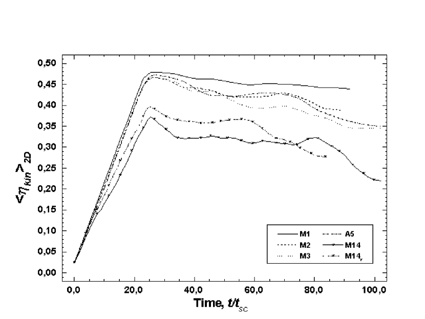
Figure 9: Time evolution of the global average of the kinetic energy fraction $\langle\eta_{kin}\rangle_{2D}$ for the runs $M1$, $M2$, $M3$, $A5$, $M14$, $M14_{r}$.

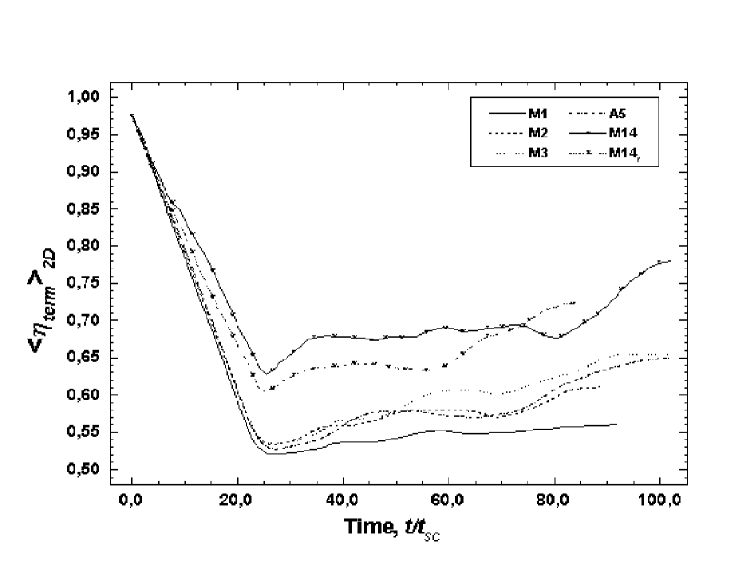
Figure 10: Time evolution of the global average of the thermal energy fraction $\langle\eta_{term}\rangle_{2D}$ for the runs $M1$, $M2$, $M3$, $A5$, $M14$, $M14_{r}$.

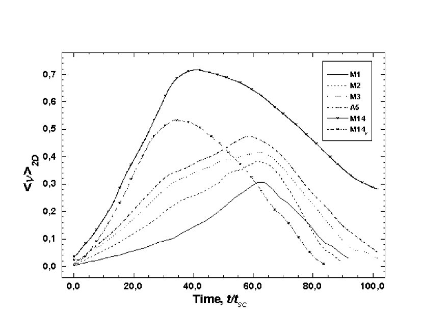
Figure 11: Time evolution of the global average of the volume filling factor $\langle\nu\rangle_{2D}$ for the runs $M1$, $M2$, $M3$, $A5$, $M14$, $M14_{r}$.

In order to characterize the global properties of the shock/cloud system interaction we plotted the time evolution of the global quantities defined in section 2.3 for the runs $M1$, $M2$, $M3$, $A5$, $M14$, and $M14_{r}$. Those plots are presented in Figures 9 - 11.

The important feature of those plots is the striking similarity of the behaviour of systems containing similar cloud distributions. The systems containing from one to five clouds arranged in a single layer exhibit exactly the same rate of momentum transfer from the global flow. This is manifested by the linear rates of fractional kinetic energy $\langle\eta_{kin}\rangle_{2D}$ increase from $t=0$ up to $t=24t_{SC}$ (see Figure 9). The value of the slope for those five cases is $0.193\pm 1.6\%$. The thermal energy $\langle\eta_{term}\rangle_{2D}$ behaves complementarily (see Figure 10). Such behavior of single layer systems contrasts that of the multiple layer systems, namely the runs $M_{14}$ and $M_{14r}$, which we now discuss.

The two fourteen cloud runs have different cloud distributions (regular as opposed to random), different total cloud mass and different cloud sizes. Nevertheless, the evolution of their fractional energies are similar. The rate of the kinetic energy increase during compression and re-expansion is the same for both $M_{14}$ and $M_{14r}$ and yet is different from that single layer cases. The slope in the multi-layer cases is also practically constant throughout the two phases with values $0.146\pm 4.5\%$.

Note that for all cases the kinetic (thermal) energy reaches its maximum (minimum) at the time $t=24t_{SC}$, or the time, defined above as the cloud destruction time $t_{CD}$, even though for the fourteen cloud runs the cloud system destruction time $t_{SD}$, defined above in subsection 3.1.3, is greater than $t_{CD}$. Thus it seems reasonable to conclude that the cloud destruction time is a universal parameter independent on the details of a cloud distribution.

After passing through its maximum, the kinetic energy fraction begins to decrease due to the transition to turbulence and, consequently, turbulent energy dissipation. It is difficult to define a value of the slope for the mixing phase due to the complex nature of the turbulent flow but the average rate of kinetic energy dissipation in the system is $\approx 0.013\pm 27\%$ for the single layer systems and $\approx 0.015\pm 25\%$ for the multiple layer ones. The proximity of these two values (within the standard error) is evidence that the systems have lost any unique details of the initial cloud distribution and developed turbulence that depends primarily on the rate of energy input at the largest scale, i.e. on the relative velocity of the global flow with respect to the cloud material.

The similarity in behaviour of single vs multiple layer systems is even more prominent in the time evolution of volume filling factors $\langle\nu\rangle_{2D}$. As can be seen in Figure 11, the rate of cloud material mixing into the global flow is the same for all single layer systems but is different from that in multiple layer ones. The higher mixing rate in the case of multiple layer distributions results because upstream clouds pick up momentum faster than the downstream ones. Upstream clouds promote destruction of the downstream ones and consequently the overall mixing of the system.

These results lead us to conclude that cloud distribution plays a more important role than the number of clouds or the total cloud mass. We use this conclusion in the next section as the foundation for classifying possible cloud distributions and defining the general type of the cloud system evolution in each category.

3.3 Critical Density Parameter

We have seen that the cloud distribution plays the defining role in determining the evolution of a shock-cloud system. We now quantify this statement and define criteria for determining the behaviour of a given system.

We define a set of all possible cloud distributions for a given number of clouds $N$. We consider only the clouds of equal or comparable size and density contrast. We define each set of cloud distributions $\lambda_{N}$ for any given number of clouds $N$ to be a set of all possible $N$ pairs of cloud center coordinates, satisfying two conditions: (1) each pair of clouds is separated by some minimum distance $r_{min}$ and (2) clouds are confined to a layer extending from the position $X_{L}$ to the position $X_{R}$ (see Figure 1):

$$\begin{array}[]{c}\forall N\geq 1:\lambda_{N}\equiv\{(x_{i},y_{i}),1\leq i\leq N\ :r_{ij}={\big{(}(x_{i}-x_{j})^{2}+(y_{i}-y_{j})^{2}\big{)}}^{\frac{1}{2}}\geq r_{min}\approx 2a_{0},\\ x_{i}\in[X_{L},X_{R}]\}.\end{array}$$ (23)

Next, we consider the complete set of all possible cloud distributions $\Lambda$ for all possible cloud numbers defined as

$$\Lambda\ =\ \displaystyle\bigcup_{N\geq 1}\{\lambda_{N}\}.$$ (24)

We define within this set $\Lambda$ the two subsets: a subset of “thin-layer” cloud distributions $\Lambda_{I}$ and a subset of “thick-layer” cloud distributions $\Lambda_{M}$ so that

$$\Lambda_{I}\ \cup\ \Lambda_{M}=\Lambda\quad and\quad\Lambda_{I}\cap\ \Lambda_{M}\ \equiv\emptyset.$$ (25)

In our numerical experiments those two subsets are associated with the single row and multiple row distributions.

In order to give a precise definition of those two fundamental classes of cloud distributions we need to introduce several auxiliary quantities.

3.3.1 Cloud Velocity and Displacement

We now estimate the distance that the cloud material will travel before the cloud breakup, i.e. within the time $t_{CD}$.

The equation of motion of a cloud in the stationary reference frame of the unshocked ambient medium takes the form

$$m_{C}\frac{dv_{C}}{dt}=\frac{1}{2}C_{D}\rho_{PS}\{v_{PS}-v_{C}\}^{2}A_{C}(t),$$ (26)

where $m_{C}$ is the mass of the cloud, $v_{C}$ is the cloud velocity in the stationary reference frame, $C_{D}$ is the cloud drag coefficient, $\rho_{PS}$ is the undisturbed postshock flow density, and $A_{C}(t)$ is the cloud cross section area normal to the flow. It should be noted that this equation is valid only until the cloud destruction is complete, i.e. until $t\approx t_{CD}$. From this point on we assume that the drag coefficient $C_{D}\approx 1$ which is a rather good approximation for a cylindrical body embedded in a supersonic flow of $M_{PS}=1.31$ (see KMC and (Bedogni & Di Fazio, 1998)).

Let us assume for a moment that the clouds have finite extent in the z-direction: $z_{0}$. Note that then

$$m_{C}=\rho_{0}\pi a_{0}^{2}z_{0},$$ (27)

where $\rho_{0}$ is the cloud density and $a_{0}$, $z_{0}$ are the cloud dimensions at time $t=0$. Moreover, the cross section area is

$$A_{C}(t)=2a_{\perp}(t)z_{0},$$ (28)

where $a_{\perp}(t)$ is the cloud radius in the direction normal to the flow. Substituting (27) and (28) into (26) and using (18) for $a_{\perp}(t)$ we get the following modified equation of motion

$$\frac{dv_{C}}{dt}=\frac{\rho_{PS}}{\rho_{0}\pi a_{0}^{2}}\{v_{PS}-v_{C}\}^{2}a_{\perp}(t).$$ (29)

This equation describes motion of the cloud as a result of its interaction with the postshock wind. However, we also need to account for the velocity that the cloud material acquires after its initial contact with the external shock front. This velocity may be comparable to the velocity acquired during the compression and re-expansion phases and, therefore, must be carefully included into consideration.

Recall that the initial contact of the incident shock front drives an internal forward shock into the cloud with velocity $v_{CS}$. Cloud material behind the internal shock front gains a velocity $v_{C,PS}$, that can be determined from the Rankine-Hugoniot relations in the usual manner,

$$v_{C,PS}=\frac{2v_{CS}}{\gamma+1}\Big{(}1-\frac{1}{M_{CS}^{2}}\Big{)}.$$ (30)

Here $M_{CS}$ is the Mach number of the cloud internal forward shock, which can be expressed in terms of the external shock Mach number as follows

$$M_{CS}=\frac{v_{CS}}{C_{C,0}}=M_{S}\Bigg{(}\frac{\gamma+1}{8/3}\Bigg{)}^{1/2}\big{(}F_{c1}F_{st}\big{)}^{1/2},$$ (31)

where by $C_{C,0}$ we denoted the sound speed in the unshocked cloud material and used (13) for $v_{CS}$. For the simulations discussed in this paper ($\chi=500$ and $\gamma=5/3$) the internal cloud shock Mach number is $M_{CS}=1.86M_{S}=18.6$.

Substituting (13) for $v_{CS}$ and (31) for $M_{CS}$ into (30), and expressing the external shock velocity $v_{S}$ in terms of the unperturbed upstream postshock velocity $v_{PS}$ by means of (6), we obtain the following expression for the velocity of the cloud material due to the cloud interaction with the external shock front

$$v_{C,PS}=v_{PS}\Bigg{(}\frac{\Big{(}\frac{\gamma+1}{8/3}\Big{)}^{1/2}\big{(}F_{c1}F_{st}\big{)}^{1/2}\Big{(}M_{S}^{2}-\frac{8/3}{\gamma+1}\big{(}F_{c1}F_{st}\big{)}^{-1}\Big{)}}{\chi^{1/2}\big{(}M_{S}^{2}-1\big{)}}\Bigg{)}=v_{PS}\Gamma.$$ (32)

For the case of $M_{S}=10$, $\Gamma=0.084$. Note that for the limiting case $M_{S}\rightarrow\infty$ the value of $\Gamma$ remains practically unchanged at $0.083$ which corroborates the previously discussed Mach scaling (see (8)).

Finally, making use of the fact that the relative velocity of the postshock flow with respect to the cloud is now $(v_{PS}-v_{C,PS}-v_{C})$, we can integrate (29) and obtain the following form of the cloud velocity

$$v_{C}(t)=\left\{\begin{array}[]{ll}\displaystyle v_{PS}\Big{(}1-\frac{1}{At+(1-\Gamma)^{-1}}\Big{)},&t\leq t_{CC}\\ \displaystyle v_{PS}\Big{(}1-\frac{1}{AB(t-t_{CC})^{2}+A(t-t_{CC})+C}\Big{)},&t_{CC}\leq t\leq t_{CD},\end{array}\right.$$ (33)

where we introduced the following quantities

$$A=\frac{\rho_{PS}v_{PS}}{\rho_{0}\pi a_{0}}=\frac{1}{t_{SC}\chi}\cdot\displaystyle\Bigg{(}\frac{\pi}{2}\Big{(}\frac{2}{\gamma+1}\bigg{(}1-\frac{1}{M_{S}^{2}}\bigg{)}\Big{)}^{-1}-1\Bigg{)}^{-1};$$ (34)

$$B=\frac{C_{C}}{2a_{0}}=\frac{1}{t_{SC}\chi^{1/2}}\cdot\big{(}F_{c1}F_{st}\big{)}^{1/2}\Bigg{(}\frac{3\gamma(\gamma-1)}{4(\gamma+1)}\Bigg{)}^{\frac{1}{2}};$$ (35)

$$C=12At_{SC}+(1-\Gamma)^{-1}.$$ (36)

The unperturbed postshock quantities $\rho_{PS}$ and $v_{PS}$ are determined from the conditions (4) and (6), $C_{c}$ is the sound speed in the shocked cloud, defined by (17), and the factor $F_{st}$ is defined by the relation (14).

The first quantity $A$ relates the specific momentum of the postshock wind to the cloud inertia (mass). Thus it defines the rate of the momentum pickup by a cloud during the compression phase, when the cloud dimension transverse to the flow does not increase. The second quantity $B$ is the inverse sound crossing time in a compressed cloud, i.e. at the end of the compression phase, again for the cloud dimension transverse to the flow. This quantity determines the rate of the cloud lateral expansion. Therefore, during the re-expansion phase the regular momentum transfer from the wind to the cloud, described by A, is augmented by the cloud lateral expansion, described by $B$, which comes as an additional factor in the quadratic dependence on $t$. Quantity $C$ ensures continuity of the cloud velocity during the transition from the compression to the re-expansion phase.

Next, integrating (33) from time $t=0.0$ up to the cloud destruction time $t=t_{CD}$ we can determine the displacement of cloud material during the compression and re-expansion phases

$$L_{C}(t)=\left\{\begin{array}[]{ll}\displaystyle v_{PS}\Bigg{(}t-\frac{1}{A}ln\Big{(}(1-\Gamma)At+1\Big{)}\Bigg{)},&0\leq t\leq t_{CC}\\ v_{PS}\displaystyle\Bigg{(}t-\frac{1}{A}\bigg{(}\frac{2}{q}tan^{-1}\frac{(t-t_{CC})q}{(t-t_{CC})+\frac{2C}{A}}+ln\Big{(}(1-\Gamma)At_{CC}+1\Big{)}\bigg{)}\Bigg{)},&t_{CC}\leq t\leq t_{CD}\end{array}\right.,$$ (37)

where $q=\sqrt{4BC/A-1}$. This allows us to estimate the total displacement a cloud incurs before its destruction, called the cloud destruction length,

$$L_{CD}=L_{C}(t_{CD}).$$ (38)

In order to get a clearer understanding of the general expressions (33) and (37) let us consider the two cases: the case presented in our simulations with $M_{S}=10$ and the limiting case of $M_{S}\to\infty$. We will assume in both cases the density contrast of $\chi=500.0$ and $\gamma=5/3$.

First, we rewrite (33) as

$$v_{C}(t)=\left\{\begin{array}[]{ll}\displaystyle v_{PS}\Bigg{(}1-\Big{(}\frac{t}{t_{SC}}a_{1}+a_{2}\Big{)}^{-1}\Bigg{)},&t\leq t_{CC}\\ \displaystyle v_{PS}\Bigg{(}1-\Big{(}\bigg{(}\frac{t}{t_{SC}}-12\bigg{)}^{2}b_{1}+\frac{t}{t_{SC}}a_{1}+a_{2}\Big{)}^{-1}\Bigg{)},&t_{CC}\leq t\leq t_{CD}\end{array}\right.$$ (39)

In the first case of $M_{S}=10$ the coefficients $a_{1}$, $a_{2}$, and $b_{1}$ have the following values

$$a_{1}\ =\ 1.79\cdot 10^{-3};\ a_{2}\ =\ 1.09;\ b_{1}\ =\ 8.35\cdot 10^{-5}.$$ (40)

Substituting these into (39) we find that at the end of the compression phase, i.e. at the time $t=12t_{SC}$, the cloud velocity is $10\%$ of the postshock velocity $v_{PS}$ and $7.5\%$ of the shock velocity $v_{S}$. On the other hand, at the end of the re-expansion phase, i.e. at the time $t=24t_{SC}$ the cloud velocity is $12.66\%$ of $v_{PS}$ and $9.4\%$ of $v_{S}$.

For the case $M_{S}\to\infty$ the above coefficients have the values

$$a_{1}\ =\ 1.83\cdot 10^{-3};\ a_{2}\ =\ 1.09;\ b_{1}\ =\ 8.51\cdot 10^{-5}.$$ (41)

Substitution into (39) gives us the maximum values of the velocity that a cloud can reach in the case of an infinitely strong shock:

$$\begin{array}[]{llllll}v_{C,max}&=&10.1\cdot 10^{-2}v_{PS}&=&7.55\cdot 10^{-2}v_{S},&compression\ phase;\\ v_{C,max}&=&12.8\cdot 10^{-2}v_{PS}&=&9.57\cdot 10^{-2}v_{S},&re-expansion\ phase.\end{array}$$ (42)

Similarly, we can determine the values of cloud displacement for the two cases, considered above. Expression (37) for $L_{C}$ can be rewritten as follows

$$L_{C}(t)=\left\{\begin{array}[]{ll}\displaystyle a_{0}c_{1}\Bigg{(}\frac{t}{t_{SC}}-\frac{1}{a_{1}}\ ln\Big{(}\frac{t}{t_{SC}}\Big{(}\frac{a_{1}}{a_{2}}\Big{)}+1\Big{)}\Bigg{)},&0\leq t\leq t_{CC}\\ \displaystyle a_{0}c_{1}\Bigg{(}\frac{t}{t_{SC}}-c_{2}\ tan^{-1}\Big{(}\frac{\frac{t}{t_{SC}}-12}{\frac{t}{t_{SC}}c_{4}+c_{5}}\Big{)}-c_{3}\Bigg{)},&t_{CC}\leq t\leq t_{CD}\end{array}\right.,$$ (43)

where for the case $M_{S}=10$ the coefficients $a_{1}$ and $a_{2}$ have the values defined in (40), and for $M_{S}\to\infty$ the values defined in (41).

In the case $M_{S}=10$ the coefficients $c_{1}$, $c_{2}$, $c_{3}$, $c_{4}$, and $c_{5}$ have the values

$$c_{1}\ =\ 1.49;\ c_{2}\ =\ 104.17;\ c_{3}\ =10.89;\ c_{4}\ =\ 9.34\cdot 10^{-2};\ c_{5}\ =\ 113.72.$$

Substitution into (43) gives us the displacement that the cloud material undergoes by the end of the compression and re-expansion phases: $1.6a_{0}$ and $3.5a_{0}$ correspondingly.

In the limiting case $M_{S}\rightarrow\infty$ the values of the coefficients $c_{1}$, $c_{2}$, $c_{3}$, $c_{4}$, and $c_{5}$ are the following

$$c_{1}\ =\ 1.5;\ c_{2}\ =\ 103.22;\ c_{3}\ =10.9;\ c_{4}\ =\ 9.43\cdot 10^{-2};\ c_{5}\ =\ 112.56.$$

Substituting these coefficients into (43) we find that by the end of the compression phase the cloud is displaced by the distance of $1.65a_{0}$, whereas by the end of the re-expansion phase the displacement is $3.53a_{0}$.

It is clear from the results, obtained above, that both the velocity and cloud displacement values in the case $M_{S}=10$ are practically identical to the maximum values, achieved in the limiting case of $M_{S}\to\infty$. Therefore, our results obtained for the case of a Mach 10 shock can be considered as the limiting ones for the cases of strong shocks.

These results, derived for single clouds or systems with large separation, are in good agreement with numerical experiments. Typically the maximum difference between numerical and analytical values of cloud velocity and position never exceeds $10\%$. The analytical results are usually an overestimate of the numerical ones. This is due to a slight overestimation of the initial velocity gain after the contact with the external shock front and because we assumed the cloud cross-section to be constant during the compression phase, whereas it undergoes a small decrease in the experiments.

Therefore, the maximum distance a cloud can travel before its destruction after the initial interaction with a strong shock is

$$L_{CD,max}\approx 3.5a_{0}.$$ (44)

3.3.2 Critical Cloud Separation

We first define the average cloud separation, projected on to the direction of the flow $\langle\Delta x_{N}\rangle$ and perpendicular to it $\langle\Delta y_{N}\rangle$, for a given cloud distribution,

$$\langle\Delta x_{N}\rangle=\frac{\displaystyle\sum_{i,j>i}^{N}|x_{i}-x_{j}|}{C_{2}^{N}}=\frac{2}{(N-1)N}\displaystyle\sum_{i,j>i}^{N}|x_{i}-x_{j}|,$$ (45)

$$\langle\Delta y_{N}\rangle=\frac{\displaystyle\sum_{i,j>i}^{N}|x_{i}-x_{j}|}{C_{2}^{N}}=\frac{2}{(N-1)N}\displaystyle\sum_{i,j>i}^{N}|y_{i}-y_{j}|.$$ (46)

We can also define a maximum cloud separation projected on to the direction of the flow, or the “cloud layer thickness”,

$$(\Delta x_{N})_{max}=\displaystyle\max_{i,j\in\{1,N\}}\{|x_{i}-x_{j}|\}.$$ (47)

Now we are in a position to give a precise definition of the “thin-layer” and “thick-layer” systems. We define a distribution of clouds to belong to the subset $\Lambda_{I}$ if its maximum cloud separation $(\Delta x_{N})_{max}$ does not exceed the cloud destruction length $L_{CD}$. The distribution belongs to the subset $\Lambda_{M}$ in all other cases:

$$\begin{array}[]{c}\Lambda_{I}\equiv\{\lambda_{N}:(\Delta x_{N})_{max}\leq L_{CD}\},\\ \Lambda_{M}\equiv\{\lambda_{N}:(\Delta x_{N})_{max}>L_{CD}\}.\end{array}$$ (48)

A more intuitive way to look at this classification is the following. As we have seen, a cloud interacting with the postshock flow re-expands and breaks up before it proceeds into the mixing phase. The above criterion tells us if any cloud or a row of clouds will complete its destruction phase prior to encountering any other clouds located downstream. The definition (48) appears to draw rather accurately the line between cloud systems of two types.

In practice the maximum cloud separation $(\Delta x_{N})_{max}$ (eq. 47) is simply the thickness of the layer of inhomogeneities in a real system and should be compared against the cloud destruction length. This thickness can be obtained from the observations of a particular object or it can be found analytically, e.g. via consideration of instabilities at the interface between two flows.

Having defined the two classes, or subsets, of cloud distributions we now consider the behaviour of the clouds in each class. First we consider $\Lambda_{I}$, the “single-row” distributions. On average, by the time the clouds are displaced by the distance $L_{CD}$, all of them will be destroyed and will proceed to the mixing phase. Thus time of the destruction should be approximately $t_{CD}\simeq t_{SD}$.

The question arises whether clouds will interact during the process of re-expansion and destruction. We can give a formal criterion for this. Consider two clouds with separation $\langle\Delta y_{N}\rangle\ =\ d$ and $(\Delta x_{N})_{max}\leq L_{CD}$. Both clouds will expand laterally at the velocity $v_{exp}$ defined in (17). Consequently the time for the clouds to come into contact is

$$t_{merge}\approx\frac{d-2a_{0}}{2v_{exp}}.$$ (49)

Such re-expansion starts after the cloud compression phase, i.e. after the time $t_{CC}$ and cannot proceed beyond the cloud destruction time $t_{CD}$. Therefore, setting $t_{merge}=t_{CD}-t_{CC}$ we find the following critical cloud separation transverse to the global flow

$$d_{crit}=2\big{(}a_{0}+v_{exp}(t_{CD}-t_{CC})\big{)}.$$ (50)

Substituting (17) explicitly for the expansion velocity and (19) for the cloud destruction time into (50) we obtain

$$d_{crit}=2a_{0}\Bigg{\{}\frac{t_{CD}-t_{CC}}{t_{SC}}\Bigg{(}\frac{F_{c1}F_{st}}{\chi}\Bigg{)}^{\frac{1}{2}}\Bigg{(}\frac{3\gamma(\gamma-1)}{\gamma+1}\Bigg{)}^{\frac{1}{2}}+1\Bigg{\}}.$$ (51)

In other words clouds whose separation transverse to the flow is less than $d_{crit}$ will come into contact and merge before their destruction is completed. Therefore, their evolution during the destruction phase (and for the most part of the re-expansion phase) can not be considered as the evolution of two independent clouds.

The critical separation does not depend on the global shock Mach number in consistency with the Mach scaling, discussed above. Therefore, this parameter is universal for all strong shocks and for all possible distributions from the subset $\Lambda_{I}$. For the case $\gamma=5/3$ and $\chi=500$ we find the critical cloud separation to be approximately

$$d_{crit}\approx 4.2a_{0}.$$ (52)

For cloud distributions from the subset $\Lambda_{I}$ which have an average separation $\langle\Delta y_{N}\rangle\gg d_{crit}$, the evolution of the system will proceed in the non-interacting regime. On the other hand, for the distributions, for which $\langle\Delta y_{N}\rangle\lesssim d_{crit}$, the cloud-cloud interactions are important throughout the re-expansion and destruction phases placing them in an interacting regime.

It is more difficult to formulate a unified criterion for the behavior of the systems in the class $\Lambda_{M}$. When $\langle\Delta x_{N}\rangle>L_{CD}$ such systems can be considered as a set of thin layers with an average separation $L_{CD}$, i.e. each row can be considered as a system from subset $\Lambda_{I}$. Consider, for example, the run $M_{14}$, presented in Figure 4. From Table (1), the average separation $\langle\Delta x_{N}\rangle$ for this run is equal to 7, i.e. $\langle\Delta x_{N}\rangle>L_{CD}$. Indeed, the evolution of the leftmost row of clouds proceeds as a simple single row case, and its destruction is completed by the time $t_{CD}$. This results in the fractional kinetic energy reaching a maximum at time $t_{CD}\approx 24t_{SC}$ (see Figure 9). However, it is clear from Figure 4 that the evolution of the downstream rows is altered by the destruction of the leftmost one. Therefore, when $\langle\Delta x_{N}\rangle>L_{CD}$ one must account for the fact that the destruction of an upstream layer of clouds will change the properties of the global flow for the next, downstream layer. The new averaged values of the velocity, density, and pressure in the global flow should then be used as an input for the analysis of the downstream cloud layer.

3.4 Mass loading

One of the principal questions concerning the effects of shock/cloud-system interactions is the role of mass-loading (Hartquist & Dyson, 1988). Mass-loading is defined as the feeding of material into the global flow by nearly stationary clouds. Analytical studies have predicted a number of important changes when mass-loading occurs. The most important of these is the transition of the flow to a transonic regime (Hartquist et al., 1986), (Hartquist & Dyson, 1988), (Dyson & Hartquist, 1992), (Dyson & Hartquist, 1994). In our numerical experiments we consider if mass-loading indeed is prominent.

Mass loading can occur only from time $t=0$ up to the moment of cloud destruction at time $t=t_{CD}$. In our experiments the cloud destruction time is fairly short compared with the total age of most relevant astrophysical objects. Indeed, cloud destruction is practically completed by the time the shock wave reaches the right boundary of the computational domain, i.e. by the time the shock wave travels the distance of about 20-30 cloud sizes. This could, for example, be compared with clump systems in planetary nebulae. Assuming typical size for PNe clouds to be about 100 a.u. (which is the size of cometary knots in NGC 7293 (Burkert & O’Dell, 1998)), a density contrast 500, and a shock wave velocity 100 km $\rm{s}^{-1}$, we find that clouds get completely destroyed within approximately $100-150$ years. This is much less than the typical age of the planetary nebulae ($10^{4}\ -\ 10^{5}$ yrs.).

Thus clouds with low density contrast $\chi_{i}\approx 10-100$ can not provide significant mass-loading due to the ease in which they are advected and destroyed by the global flow. On the other hand, clouds with higher density contrasts $\chi_{i}>100$ retain their low velocities with respect to the global flow for much longer periods of time and, therefore, may potentially be efficient mass-loading sources. However, it should be noted, that this higher relative velocity of a cloud increases the efficiency of the instability formation, thereby promoting cloud destruction and its mixing with the flow.

We can also consider the amount of mass seeded into the flow, i.e. stripped of from the clouds and assimilated into the global flow, before cloud destruction. Typically, in our experiments the amount of seeded cloud material does not exceed a few percent of the total cloud mass, which is unlikely to be enough to switch the flow into a mass-loaded regime. Figure 12 shows the distribution of cloud material along the direction of the flow or, to be more precise, the distribution of the parameter $\langle\nu\rangle_{1D}(x)$ for the three cloud run $M_{3}$. There the clouds have the separation $\langle\Delta y_{N}\rangle\approx 0.95d_{crit}$. The first graph corresponds to the end of the compression phase, while the second corresponds to the end of the destruction phase. The graphs show that cloud material remains localized in the vicinity of the cloud cores until the moment of cloud destruction and the system does not exhibit any significant mass-loading. Moreover, the graphs 3 and 4 of Figure 12, showing cloud material distribution early in the mixing phase, indicate that even after destruction cloud material remains localized within the region of about 8 cloud radii and retains almost the same average velocity with respect to the global flow. Only further on in the mixing phase does cloud material spread significantly.

Concluding, we may say that for the cloud density contrast values in the range $\chi_{i}\approx 10-1000$ and practically all values of the global shock wave Mach number, the flows are not likely to be subject to mass loading. These flows will be dominated by the mixing of cloud material with the global flow that occurs after cloud destruction. Systems with very dense clouds $\chi_{i}>>1000$ may provide sites suitable for mass loading. Future numerical studies should be able to confirm this.

4 CONCLUSIONS

We have numerically investigated the interaction of a strong, planar shock wave with a system of inhomogeneities. These ”clumps” are considered to be infinitely long cylinders embedded in a tenuous, cold ambient medium. We have assumed constant conditions in the global postshock flow, thereby constraining the maximum size of the clouds only by the condition of the shock front planarity. Our results are applicable to strong global shocks with Mach numbers $3\lesssim M_{S}\lesssim 1000$. The range of the applicable cloud/ambient density contrast values is $10-1000$.

We considered four major phases of the cloud evolution due to the interaction of the global shock and postshock flow with a system of clouds. These are: initial compression phase, re-expansion phase, destruction phase, and mixing phase. We describe a simple model for the cloud acceleration during the first three phases, i.e. prior to its destruction, and derive expressions for the cloud velocity and displacement. The results of that model are in excellent agreement with the numerical experiments. The difference in the values of cloud velocity and displacement between analytical and numerical results is $\lesssim 10\%$. The maximum cloud displacement due to its interaction with a strong shock (prior to its destruction) does not exceed $3.5$ initial maximum cloud radii. The maximum cloud velocity is not more than $10\%$ of the global shock velocity.

The principal conclusion of the present work is that the set $\Lambda$ of all possible cloud distributions can be subdivided into two large subsets $\Lambda_{I}$ and $\Lambda_{M}$. The first subset is $\Lambda_{I}$, thin-layer systems. This subset is defined by the condition that the maximum cloud separation along the direction of flow, or the cloud layer thickness, is not greater than the cloud destruction length $(\Delta x_{N})_{max}\leq L_{CD}$. The thick-layer systems $\Lambda_{M}$, are defined by the condition $(\Delta x_{N})_{max}>L_{CD}$. The evolution of cloud distributions within each subset exhibit striking similarity in behaviour. We conclude that the evolution of a system of clouds interacting with a strong shock depends primarily on the total thickness of the cloud layer and the cloud distribution in it, as opposed to the total number of clouds or the total cloud mass present in the system. The key parameters determining the type of the cloud system evolution are therefore the critical cloud separation transverse to the flow $d_{crit}$ (this is also the critical linear cloud density in the layer), and the cloud destruction length $L_{CD}$.

For a given astrophysical situation our results indicate that one might determine, either from observations or from theoretical analysis, the thickness of the cloud layer $(\Delta x_{N})_{max}$. This will then determine the class of the given cloud distribution, $\Lambda_{I}$ or $\Lambda_{M}$. For cloud distributions from the set $\Lambda_{I}$ with average cloud separation $\langle\Delta y_{N}\rangle>d_{crit}$ evolution of the clouds during the compression, re-expansion, and destruction phases will proceed in the noninteracting regime and the formalism for a single cloud interaction with a shock wave (e.g. KMC, (Jones et al., 1996), (Mac Low et al., 1994), (Lim & Raga, 1999)) can be used to describe the system. On the other hand, if the cloud separation is less than the critical distance, the clouds in the layer will merge into a single structure before their destruction is completed. Though throughout the compression phase they can still be considered independently of each other, their evolution during the re-expansion and destruction phases clearly proceeds in the interacting regime.

When the distribution belongs to the subset $\Lambda_{M}$ it is necessary to determine the average cloud separation projected onto the direction of the flow $\langle\Delta x_{N}\rangle$, defined by (45) above, and compare it against $L_{CD}$: if $\langle\Delta x_{N}\rangle>L_{CD}$ evolution of the cloud system can be roughly approximated as the evolution of a set of distributions from the subset $\Lambda_{I}$ and the above “thin-layer case” analysis applies. If, on the other hand, $\langle\Delta x_{N}\rangle\leq L_{CD}$ (especially if $\langle\Delta y_{N}\rangle<d_{crit}$) the system evolution is dominated by cloud interactions and a thin layer formalism is inappropriate.

Finally we have considered the role of mass-loading. Here our principal conclusion is that the mass-loading is not significant in the cases of strong shocks interacting with a system of inhomogeneities for density contrasts in the range $10-1000$. In part this is due to short survival times of clouds under such conditions, and in part due to the very low mass loss rates of the clouds even during the times prior to their destruction. Mass loading may well be important in higher density clouds (Dyson & Hartquist, 1994).

The major limitation of our current work is the purely hydrodynamic nature of our analysis that does not include any consideration of magnetic fields. As it was discussed in section 3.1.4, cold dense inhomogeneities (clouds) embedded in tenuous hotter medium are inherently unstable against the dissipative action of diffusion and thermal conduction. This evaporates the clouds on the timescales comparable to, or shorter than, the timescales of the dynamical evolution of the system. It was suggested that the magnetic fields may play a stabilizing role against the action of the dissipative mechanisms. Although weak magnetic fields, that are dynamically insignificant up to the moment of cloud destruction, can inhibit thermal conduction and diffusion, those magnetic fields may become dynamically important due to turbulent amplification during the mixing phase. A fully magnetohydrodynamic description of the interaction of a strong shock with a system of clouds will need to be carried forward in future works.

Table 1: Summary of the Runs Discussed

Run	$\#$ of clouds	Distribution	$\#$ of rows	x-spacing	y-spacing
M1	1	regular	1	-	-
M2	2	regular	1	-	4
A2	2	regular	1	-	12
M3	3	regular	1	-	4
A5	5	regular	1	-	4
M14	14	regular	3	7	4
$M14_{r}$	14	random	3	3.5	3.5

Figure 1: Setup of the computational domain. Shown is the setup for the run $M14$. “x-spacing” and “y-spacing” are the parameters used in Table 1 for the description of the runs. Note: not drawn to scale.

Figure 2: Run $M1$. Time evolution of a system, containing a single cloud and interacting with a $M_{S}=10$ shock wave. Shown are the synthetic Schlieren images of the system at times $22.47\ t_{SC}$, $35.23\ t_{SC}$, $50.54\ t_{SC}$, $68.40\ t_{SC}$.

Figure 3: Run $M3$. Time evolution of a system, containing three identical clouds and interacting with a $M_{S}=10$ shock wave. Shown are the synthetic Schlieren images of the system at times $22.47\ t_{SC}$, $35.23\ t_{SC}$, $50.54\ t_{SC}$, $68.40\ t_{SC}$.

Figure 4: Run $M14$. Time evolution of a system, containing fourteen identical clouds in a regular distribution and interacting with a $M_{S}=10$ shock wave. Shown are the synthetic Schlieren images of the system at times $22.47\ t_{SC}$, $35.23\ t_{SC}$, $50.54\ t_{SC}$, $69.09\ t_{SC}$.

References

- Anderson et al. (1994) Anderson, M.C., Jones, T.W., Rudnick, L., Tregillis, I.L., Kang, H. 1994, ApJ, 421, L31
- Arthur et al. (1996) Arthur, S.J., Henney, W.J., Dyson, J.E. 1996, A&A, 313, 897
- Bedogni & Di Fazio (1998) Bedogni, R., Di Fazio, A. 1998, Nuovo Cimento, 113 B, 1373
- Berger & Colella (1989) Berger, M.J., Colella, P. 1989, J. Comp. Phys., 82, 64
- Berger & Jameson (1985) Berger, M.J., Jameson, A. (1985), AIAA J., 23, 561
- Berger & LeVeque (1997) Berger, M.J., LeVeque, R.J. 1998, SIAM J. Numer. Anal., 35, 2298
- Berger & Oliger (1984) Berger, M.J., Oliger, J. 1984, J. Comp. Phys., 53, 484
- Burkert & O’Dell (1998) Burkert, A., O’Dell, C.R. 1998, ApJ, 503, 792
- Chandrasekhar (1961) Chandrasekhar, S. 1961, Hydrodynamic and Hydromagnetic Stability (New York:Dover)
- Dyson & Hartquist (1992) Dyson, J.E., Hartquist, T.W. 1992, ApL, 28, 301
- Dyson & Hartquist (1994) Dyson, J.E., Hartquist, T.W. 1994, in 34th Herstmonceux Conf., Circumstellar Media in the Late Stages of Stellar Evolution, eds. R. Clegg, P. Meikle, & I. Stevens (Cambridge: CUP)
- Gregori et al. (1999) Gregori, G., Miniati, F., Ryu, D., Jones, T.W. 1999, ApJ, 527, L113
- Gregori et al. (2000) Gregori, G., Miniati, F., Ryu, D., Jones, T.W. 2000, ApJ, 543, 775
- Hartquist & Dyson (1988) Hartquist, T.W., Dyson, J.E. 1988, Ap&SS, 144, 615
- Hartquist et al. (1986) Hartquist, T.W., Dyson, J.E., Pettini, M., Smith, L.J. 1986, MNRAS, 221, 715
- Hartquist et al. (1997) Hartquist, T.W., Dyson, J.E., Williams, R.J.R. 1997, ApJ, 482, 182
- Hornung (1986) Hornung, H. 1986, Ann. Rev. Fluid Mech., 18, 33
- Jones et al. (1996) Jones, T.W., Ryu, D., Tregillis, I.L. 1996, ApJ, 473, 365
- Jun & Jones (1999) Jun, B.-I., Jones, T.W. 1999, ApJ, 511, 774
- Jun et al. (1996) Jun, B.-I., Jones, T.W., Norman, M.L. 1996, ApJ, 468, L59
- Klein et al. (1994) Klein, R.I., McKee, C.F., Colella, P. 1994, ApJ, 420, 213
- Kuncic et al. (1996) Kuncic, Z., Blackman, E.G., Rees, M.J. 1996, MNRAS, 283, 1322
- Landau & Lifshitz (1959) Landau, L.D., Lifshitz, E.M. 1959, Fluid Mechanics (Reading:Addison-Wesley)
- LeVeque (1997) LeVeque, R.J. 1997, J. Comp. Phys., 131, 327
- Lim & Raga (1999) Lim, A.J., Raga, A.C. 1999, MNRAS, 303, 546
- Mac Low et al. (1994) Mac Low, M.-M., McKee, C., Klein, R., Stone, J.M., Norman, M.L. 1994, ApJ, 433, 757
- Miller & Bailey (1979) Miller, D.G., Bailey, A.B. 1979, J. Fluid Mech., 93, 449
- Miniati et al. (1999) Miniati, F., Jones, T.W., Ryu, D. 1999, ApJ, 517, 242
- O’Dell et al. (1990) O’Dell, C.R., Weiner, L.D., Chu, Y.-H. 1990, ApJ, 362, 226
- Phillips & Cuesta (1999) Phillips, J.P., Cuesta, L. 1999, ApJ, 118, 2929
- Poludnenko et al. (2001) Poludnenko, A.Y., Frank, A., Blackman, E.G. 2001, in ASP Conf. Ser., The Mass Outflow in Active Galactic Nuclei: New Perspectives, ed. D.M. Crenshaw, S.B. Kraemer, & I.M. George (San Francisco:ASP), in press
- Redman et al. (1998) Redman, M.P., Williams, R.J.R., Dyson, J.E. 1998, MNRAS, 298, 33