Physics of Cosmic Microwave Background Anisotropies and Primordial Fluctuations

Abstract

The physics of the origin and evolution of CMB anisotropies is described, followed by a critical discussion of the present status of cosmic parameter estimation with CMB anisotropies.

1 Introduction

The discovery of anisotropies in the cosmic microwave background (CMB) by the COBE satellite in 1992 [22, 2] has stimulated an enormous activity in this field which has culminated recently with the high precision data of the BOOMERanG, MAXIMA-I and DASI experiments [5, 11, 17, 15, 10]. The CMB is developing into the most important observational tool to study the early Universe. Recently, CMB data has been used mainly to determine cosmological parameters for a fixed model of initial fluctuations, namely scale invariant adiabatic perturbations. In my talk I outline this procedure and present some results. I will also mention the problem of degeneracies and indicate how these are removed by measurements of the CMB polarization or other cosmological data. Finally, I include a critical discussion of the model assumptions which enter the parameter estimations and will show in an example what happens it these assumptions are relaxed.

In the next section we discuss in some detail the physics of the CMB. Then we investigate how CMB anisotropies depend on cosmological parameters. We also discuss degeneracies. In Section 4 we investigate the model dependence of the ’parameter estimation’ procedure. We end with some conclusions.

2 The physics of the CMB

Before discussing the possibilities and problems of parameter estimation using CMB anisotropy data I want to describe the physics of these anisotropies. As CMB anisotropies are small, they can be treated nearly completely within linear cosmological perturbation theory. Effects due to non-linear clustering of matter, like e.g. the Rees-Sciama effect, the Sunyaev-Zel’dovich effect or lensing are relevant only on very small angular scales ($\ell\stackrel{{\scriptstyle>}}{{\sim}}1000$) and are not discussed here.

Since the CMB anisotropies are a function on a sphere, they can be expanded in spherical harmonics,

$${\Delta T\over T_{0}}({\bf n})=\sum_{\ell=1}^{\infty}\sum_{m=-\ell}^{m=\ell}a_{\ell m}Y_{\ell m}({\bf n})~{},$$ (1)

where $\Delta T=T-T_{0}$ and $T_{0}$ is the mean temperature on the sky. The CMB power spectrum $C_{\ell}$ is the ensemble average of the coefficients $a_{\ell m}$,

$$C_{\ell}=\langle|a_{\ell m}|^{2}\rangle~{}.$$

If the fluctuations are statistically isotropic, the $C_{\ell}$’s are independent of $m$ and if they are Gaussian all the statistical information is contained in the power spectrum. The relation between the power spectrum and the two point correlation function is given by

$$\left\langle{\Delta T\over T_{0}}({{\bf n}_{1}}){\Delta T\over T_{0}}({{\bf n}_{2}})\right\rangle={1\over 4\pi}\sum_{\ell}(2\ell+1)C_{\ell}P_{\ell}({\bf n}_{1}\cdot{\bf n}_{2})~{}.$$ (2)

In a real experiment, unfortunately, we have only one universe and one sky at our disposition and can therefore not measure an ensemble average. In general, one assumes statistical isotropy and sets

$$C_{\ell}\simeq C_{\ell}^{obs}={1\over 2\ell+1}\sum_{m}|a_{\ell m}|^{2}~{}.$$

In the ideal case of full sky coverage, this yields an average on $2\ell+1$ numbers (note that $a_{\ell m}=a_{\ell-m}^{*}$). If the temperature fluctuations are Gaussian, the observed mean deviates from the ensemble average by about

$${\sqrt{(C_{\ell}^{obs}-C_{\ell})^{2}}\over C_{\ell}}\simeq\sqrt{2\over 2\ell+1}~{}.$$ (3)

This fundamental limitation of the precision of a measurement which is important especially for low multipoles is called cosmic variance. In practice one never has complete sky coverage and the cosmic variance of a given experiment is in general substantially larger than the value given in Eq. (3).

Within linear perturbation theory one can split perturbations into scalar, vector and tensor contributions according to their transformation properties under rotation. The different components do not mix. Initial vector perturbations rapidly decay and are thus usually neglected. Scalar and tensor perturbations contribute to CMB anisotropies. After recombination of electrons and protons into neutral hydrogen, the universe becomes transparent for CMB photons and they move along geodesics of the perturbed Friedman geometry. Integrating the perturbed geodesic equation, one obtains the following expressions for the temperature anisotropies of scalar ($s$) and tensor ($t$) perturbations

$$\left({\Delta T\over T}\right)^{(s)}(\eta_{0},{\bf x}_{0},{\bf n}) = {1\over 4}D_{r}(\eta_{dec},{\bf x}_{dec})+v_{i}(\eta_{dec},{\bf x}_{dec})n^{i}+(\Phi-\Psi)(\eta_{dec},{\bf x}_{dec})$$ (4)

$$-\int_{\eta_{dec}}^{\eta_{0}}(\dot{\Phi}-\dot{\Psi})(\eta,{\bf x}(\eta))d\eta~{},$$

$$\left({\Delta T\over T}\right)^{(t)}(\eta_{0},{\bf x}_{0},{\bf n}) = -\int_{\eta_{dec}}^{\eta_{0}}\dot{h}_{ij}(\eta,{\bf x}(\eta))n^{i}n^{j}d\eta~{}.$$ (5)

Here $\eta$ denotes conformal time, $\eta_{0}$ indicates today while $\eta_{dec}$ is the time of decoupling ($z_{dec}\sim 1100$) and ${\bf x}(\eta)$ is the comoving unperturbed photon position at time $\eta$, ${\bf x}(\eta)={\bf x}_{0}-{\bf n}(\eta-\eta_{0})$ for a flat universe, ${\bf x}_{dec}={\bf x}(\eta_{dec})$. The above expression for the temperature anisotropy is written in gauge-invariant form [7]. The variable $D_{r}$ represents the photon energy density fluctuations, $v_{i}$ is the baryon velocity field and $\Phi$ and $\Psi$ are the Bardeen potentials, the scalar degrees of freedom for metric perturbations of a Friedman universe [1]. For perturbations coming from ideal fluids or non-relativistic matter $\Psi=-\Phi$ is simply the Newtonian gravitational potential.

2.1 The Sachs Wolfe effect

On large angular scales, the dominant contributions to the power spectrum for scalar perturbations come from the first term and the Bardeen potentials. The integral is often called the ’integrated Sachs Wolfe effect’ (ISW) while the first and third terms of Eq. 4 are the ’ordinary Sachs Wolfe effect’ (OSW). In the general case this split is purely formal, but in a matter dominated universe with critical density, $\Omega_{m}=1$, the Bardeen potentials are time independent and the ISW contribution vanishes.

For adiabatic fluctuations in a matter dominated universe, one has ${1\over 4}D_{r}={1\over 3}D_{m}={5\over 3}\Psi$. Together with $\Phi=-\Psi$ this yields the original formula of Sachs and
Wolfe (1967):

$$\left({\Delta T\over T}\right)^{SW}=-{1\over 3}\Psi~{}.$$

Tensor perturbations (gravity waves) only contribute on large scales, where metric perturbations are most relevant. Note the similarity of the tensor contribution to the ISW term which has the same origin.

2.2 Acoustic oscillations and the Doppler term

Prior to recombination, photons, electrons and baryons form a tightly coupled fluid. On sub-horizon scales this fluid performs acoustic oscillations driven by the gravitational potential. The wave equation in Fourier space is

$$\dot{D}+3(c_{s}^{2}-w){\dot{a}\over a}D+(1+w)k^{2}V = 0$$ (6)

$$\dot{V}+{\dot{a}\over a}(1-3c_{s}^{2})V-{c_{s}^{2}\over w+1}D = \Psi-3c_{s}^{2}\Phi$$ (7)

where $w=p/\rho$ and $c_{s}^{2}={\dot{p}/\dot{\rho}}$ is the adiabatic sound speed. Since before recombination, the baryon photon fluid is dominated by radiation we have $w\simeq c_{s}^{2}\simeq 1/3$.The system (6,7), which is a pure consequence of energy momentum conservation for the baryon photon fluid, can be combined to a second order wave equation for $D$. On very large, super-horizon scales, $k\eta\ll 1$ the oscillatory term can be neglected and $D$ remains constant. Once $k\eta\stackrel{{\scriptstyle>}}{{\sim}}1$ $D$ begins to oscillate like an acoustic wave. For pure radiation, $c_{s}^{2}=w=1/3$ the damping term vanishes and the amplitude of the oscillations remains constant. At late times there is a slight damping of the oscillations.

If adiabatic perturbations have been created during an early inflationary epoch, the waves are in a maximum as long as $k\eta\ll 1$ and perturbations with a given wavenumber all start oscillating in phase. At the moment of recombination, when the photons become free and the acoustic oscillations stop, the perturbations of a given wave length thus have all the same phase. As each given wave length is projected to a fixed angular scale on the sky, this leads to a characteristic series of peaks and troughs in the CMB power spectrum. The first two terms in Eq. (4) are responsible for these acoustic peaks.

In Fig. 1 we show the density and the velocity terms as well as their sum. The density term is often called the ’acoustic term’ while the velocity term is the ’Doppler term’. It is clearly wrong to call the peaks in the CMB anisotropy spectrum ’Doppler peaks’ as the Doppler term actually is close to a minimum at the position of the peaks! We therefore call them acoustic peaks.

Figure 1: The contribution from the photon density fluctuations ($D_{r}$-term, dashed line), from the Doppler term (${\bf v}\cdot{\bf n}$, dotted line) and their sum (solid line) are shown. The peaks clearly follow the acoustic contribution while the Doppler term dominates in the first few minima. Silk damping is not included here.

2.3 Silk damping

So far we have neglected that the process of recombination takes a finite amount of time and the ’surface of last scattering’ has a finite thickness. In reality the transition from perfect fluid coupling with a very short mean free path to free photons with mean free path larger than the size of the horizon takes a certain time during which photons can diffuse out of over–densities into under–densities. This diffusion damping or Silk damping [21] exponentially reduces CMB anisotropies on small scales corresponding to $\ell\stackrel{{\scriptstyle>}}{{\sim}}800$. The precise damping scale depends on the amount of baryons in the universe.

In addition to Silk damping, the finite thickness of the recombination shell implies that not all the photons in the CMB have been emitted at exactly the same moment and therefore we do not see all the fluctuations precisely in phase. This ’smearing out’ also leads to damping of CMB anisotropies on about the same angular scale as Silk damping.

To calculate these phenomena with good precision one has to compute the process of recombination numerically and integrate the photon Boltzmann equation. Since a couple of years there are public codes available [20, 16] which compute the CMB anisotropies numerically with a precision of about $1$%.

2.4 Polarization

There is an additional phenomenon which we have not considered so far: Non-relativistic Thompson scattering, which is the dominant scattering process on the surface of last scattering, is anisotropic. The scattering cross section for photons polarized in the scattering plane is [13]

$$\sigma_{//}={3\sigma_{T}\over 8\pi}\cos^{2}\theta~{},$$

while the cross section for photons polarized normal to the plane is

$$\sigma_{\perp}={3\sigma_{T}\over 8\pi}~{}.$$

Here $\sigma_{T}$ is the Thomson cross section and $\theta$ is the scattering angle. Therefore, even if the incoming radiation is completely unpolarized, if its intensity is not perfectly isotropic (actually if it has a non-vanishing quadrupole) the outgoing radiation will be linearly polarized. There exist two types of polarization signals: the so called $E$-type polarization which has positive parity, and $B$-type polarization which is parity odd. Scalar perturbations only produce $E$-type polarization, while tensor perturbations, gravity waves, produce both, $E$- and $B$-type. Thomson scattering never induces circular polarization.

A more detailed treatment of polarization of CMB anisotropies can be found e.g. in [12]. A typical CMB anisotropy and polarization spectrum as it is expected from inflationary models is shown in Fig. 2. Polarization of the CMB has not yet been observed. The best existing limits are on the order of a few$\times 10^{-6}$. There is hope that the next Boomerang flight (planned for December 2001) or the MAP satellite [25], which has been launched successfully in June 2001, will detect polarization.

Figure 2: The scalar (left) and tensor (right) CMB anisotropy and polarization spectra. Solid lines show the temperature anisotropy, dashed lines $E$-polarization and dotted lines $B$-polarization. The thick lines represent a model with critical density, $\Omega_{0}=1$ while the thin lines come from an open model, $\Omega_{0}=0.4$. The normalization is arbitrary. Figure from Hu et al. (1998).

3 Cosmological parameters and degeneracy

In the simplest models for structure formation where adiabatic Gaussian perturbations are created during an inflationary phase, initial perturbations are characterized by two to four numbers: The amplitudes and spectral indices of scalar and tensor perturbations. Apart from these data characterizing the initial conditions, the resulting CMB anisotropies depend only on the cosmological parameters of the underlying model, the matter density parameter, $\Omega_{m}$, the cosmological constant, $\Omega_{\Lambda}$, curvature, $\Omega_{K}=1-\Omega_{0}$, the Hubble parameter, $h=H_{0}/(100{\rm km/s/Mpc})$, the (reduced) baryon density $\omega_{b}=\Omega_{b}h^{2}$, the reionization history, which is usually cast into an effective depth to the last scattering surface, $\tau_{c}$, and a few others. Therefore, if the model of structure formation is a simple adiabatic inflationary model, CMB anisotropies can be used to determine cosmological parameters. The presently available data have been used for this goal in numerous papers and slightly different approaches have led to slightly different but, within the still considerable error bars, consistent results (see e.g. [5, 18, 14] and many others). As an example we show the results of de Bernardis et al. (2001). In Fig. 3 the likelihood functions for the total density parameter, $\Omega_{0}$, the scalar spectral index, $n_{s}$, and the baryon density, $\omega_{b}$, as obtained from the COBE DMR and the BOOMERANG data are shown [6]. An adiabatic model with purely scalar perturbations, with $0.45<h<0.95$ and with an age larger than 10Gyr has been assumed for the determination of the likelihoods. The solid lines, which have been obtained by marginalization over all the parameters not shown on the panel, are the most relevant. They imply $\Omega_{0}=1.02\pm 0.06$, $n_{s}=1.02\pm 0.1$ and $\omega_{b}=0.024\pm 0.005$. The latter value coincides most remarkably with the completely independent determination from nucleosynthesis result [4] which yields $\omega_{b}=0.019\pm 0.02$.

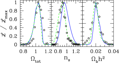
Figure 3: The likelihood curves derived from the BOOMERANG and COBE/DMR data sets for the variables $\Omega_{tot}=\Omega_{0}$, $n_{s}$ and $\Omega_{b}h^{2}=\omega_{b}$ for a model with purely scalar adiabatic fluctuations are shown. The solid lines are marginalized over the other variables while for the dashed lines (and the open circles) the maximum likelihood point in the other variables is chosen; from de Bernardis et al. (2001).

The most interesting outcome from these parameter estimations is that if initial perturbations are adiabatic, the Universe is very close to flat. Together with the cluster data which indicate $0.1\leq\Omega_{m}\leq 0.3$ this suggests, completely independent from the supernova results, that the density of the universe is dominated by a non-clustered form of dark energy, e.g. a cosmological constant with $\Omega_{\Lambda}\sim 0.7$.

However promising this procedure is, it is important to keep in mind that there are certain exact degeneracies in the CMB data which cannot be removed by CMB data alone. Let us consider, for example, the parameters $\Omega_{m},\Omega_{\Lambda},\Omega_{b},h$. Apart from the ISW contribution which is relevant only at low values $\ell$ where cosmic variance prohibits a precise determination, the CMB anisotropies depend on these parameters only via the baryon density, $\omega_{b}$, the matter density $\omega_{m}=\Omega_{m}h^{2}$ and the angular diameter distance given by $d_{dec}=\chi(\eta_{0}-\eta_{dec})$, where

$$\chi(y)=\left\{\begin{array}[]{ll}\sin(y)&\mbox{ if }~{}~{}K>0\\ \sinh(y)&\mbox{ if }~{}~{}K<0\\ y&\mbox{ if }~{}~{}K=0,\end{array}\right.$$

and

$$y=\eta_{0}-\eta_{\rm dec}=\sqrt{|\Omega_{K}|}\int_{0}^{z_{dec}}{dz\over[\Omega_{m}(1+z)^{3}+\Omega_{K}(1+z)^{2}+\Omega_{\Lambda}]^{1/2}}.$$

The CMB anisotropies for $\ell\stackrel{{\scriptstyle>}}{{\sim}}50$ only depend on the following three combinations of the four parameters considered: $R\equiv d_{dec}(\Omega_{\Lambda}=0,\Omega_{m}=1)/d_{dec}(\Omega_{\Lambda}=0,\Omega_{m}),~{}\omega_{b}$ and $\omega_{m}$. In Fig. 4 lines of constant $R$ are indicated in the $\Omega_{\Lambda}$–$\Omega_{m}$ plane.

Figure 4: left: The lines of constant $R$ are shown in the $\Omega_{\Lambda}$–$\Omega_{m}$ plane. The values $\Omega_{\Lambda},\Omega_{m}$ for which the CMB anisotropy spectra are shown right are indicated as black dots.                            right:Three CMB anisotropy spectra with different values of $\Omega_{\Lambda}$ and $\Omega_{m}$ but fixed $R$ are shown. For $\ell\stackrel{{\scriptstyle>}}{{\sim}}50$ these spectra are clearly degenerate.The solid line represents a flat model, while the dotted line corresponds to a closed and the dashed line to an open universe, from Trotta (2001).

The degeneracy is shown in Fig. 4 for a fixed value of $R$ but different points in the $\Omega_{\Lambda}$–$\Omega_{m}$ plane.

It is hence not possible to determine all four parameters $\Omega_{m},\Omega_{\Lambda},\Omega_{b},h$ with good accuracy from CMB data alone. There exist also other degeneracies, e.g. between the spectral index and the epoch of reionization or the amplitude of tensor perturbations.

We therefore consider it very important that CMB anisotropy measurements are complemented with other, more direct methods to measure cosmological parameters so that this degeneracies are broken, and also to obtain a comfortable degree of redundancy.

4 Model dependence

Apart from the degeneracies mentioned in the previous section, the cosmological parameters inferred form CMB anisotropies very strongly depend on the model assumptions. For example, in the case of isocurvature instead of adiabatic initial perturbations, for a model with critical density the first acoustic peak is at $\ell\sim 350$, and a peak at $\ell\sim 210$ indicates a closed universe. However, a closed model with isocurvature perturbations has acoustic peaks which are narrower and more closely spaced than those seen in the data. One such model, together with the data, is shown in Fig. 5. More details can be found in [8, 9].

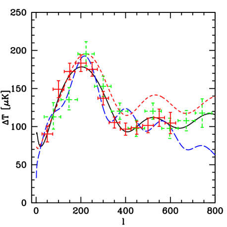
Figure 5: CMB anisotropies for three different models are shown, together with the Boomerang (solid, red) and Maxima (dashed, green) data. The short dashes show a standard adiabatic inflationary model, the long dashes show a closed isocurvature model, while the solid line shows another so called ’scaling seed’ model. Figure from Durrer et al. (2001b).

Very generic initial conditions for a universe with dark matter, photons, baryons and neutrinos are combinations of the adiabatic mode and four different isocurvature modes which may or may not be correlated [3]. The initial conditions are then specified by a $5\times 5$ positive definite matrix, the correlation matrix of the different modes. It is interesting to compare parameter estimation when allowing for this more generic initial conditions to the parameters obtained from the data when allowing only for the adiabatic mode. As an example we show the confidence ranges in the $h,\omega_{b}$ plane for both cases in Fig. 6 (see Trotta et al. (2001)).

     

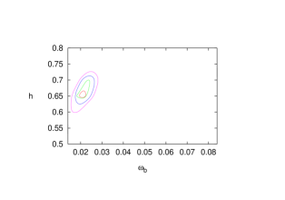
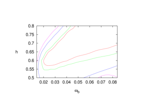
Figure 6: The $h,\omega_{b}$ confidence contours as obtained from the Boomerang data [17], when allowing only for the adiabatic mode (left) and when allowing for a general correlated mixture of the adiabatic and isocurvature modes (right). Figure from Trotta et al. (2001).

Clearly, once allowing for isocurvature modes one cannot obtain anymore reasonable upper limits for $\omega_{b}$ or $h$. What I find even more interesting here is that once we require $\omega_{b}\sim 0.02\pm 0.002$ due to the nucleosynthesis constraint and $h\sim 0.65\pm 0.1$ as favored by several independent estimates, we find that the isocurvature content in the initial conditions has to be relatively modest, $\stackrel{{\scriptstyle<}}{{\sim}}30$%.

Nevertheless, I believe that the above makes it clear that estimation of cosmic parameters by CMB anisotropies is strongly model dependent.

5 Conclusions

In this talk I have discussed the physics of CMB anisotropies and what we can learn from them. I have been relatively critical in my account of cosmic parameter estimation from CMB anisotropies. This because in the very abundant literature on the subject, little emphasis is given on the model dependence of this way of ’measuring’ cosmological parameters. Clearly every measurement in physics and even more so in cosmology depends on the underlying theory. But usually the theory has been tested before in many different setups, while in cosmology, CMB anisotropies are probably the best experimental data to test theories for cosmological initial perturbations, i.e. to investigate cosmological perturbations at a very early stage. Therefore I find it to some extent a waste if one uses these data simply to determine a few numbers which can also be measured much more directly (e.g. by kinematic measurements with SNeIa’s).

On the other hand, it is intriguing how well the present CMB data can be fit by the simplest adiabatic model of scalar perturbations with cosmological parameters well within the range obtained by other measurements.

I thank the organizer of the workshop for providing such an interesting conference and a stimulating atmosphere for discussions. I have profited from many discussions with colleagues, especially Paolo de Bernardis, Pedro Ferreira, Martin Kunz, Alessandro Melchiorri, Alain Riazuelo, Roberto Trotta and Neil Turok. I’m grateful to Norbert Straumann for carefully reading the first version of this contribution. I also thank the Institute for Advanced Study, where this paper was completed, for hospitality.

References

- [1] Bardeen, J.M.: 1980, ’Gauge invariant cosmological perturbations’ Phys. Rev. D22 1882–1905.
- [2] Bennett, C.L. et al.: 1996, ’4-Year COBE DMR microwave background observations: maps and basic results’ Astrophys. J. Lett. 464, L1–L4 .
- [3] Bucher, M. Moodley, K. and Turok, N.: 2000, ’The general primordial cosmic perturbation’. Phys. Rev. D62 083508.
- [4] Burles, S. Nollet, K.M and Turner, M.S.: 2001, ’Big-Bang nucleosynthesis predictions for precision cosmology’. Astrophys. J. Lett. 552, L1–L6
- [5] de Bernardis, P. et al.: 2000, ’A flat Universe from high-resolution maps of the cosmic microwave background radiation’. Nature 404, 922–925.
- [6] de Bernardis, P. et al.: 2000, ’Multiple peaks in the angular power spectrum of the cosmic microwave background: significance and consequences for cosmology’. Preprint astro-ph/0105296.
- [7] Durrer, R. : 1990, ’Gauge invariant cosmological perturbation theory with seeds’. Phys. Rev. D42 2533-2541.
- [8] Durrer, R., Kunz, M. and Melchiorri, A. : 2001, ’Reproducing the observed cosmic microwave background anisotropies with causal scaling seeds’. Phys. Rev. D63 081301.
- [9] Durrer, R., Kunz, M. and Melchiorri, A. : 2001, ’Cosmic structure formation with topological defects’. Phys. Rep. in print.
- [10] Halverson, N.W. et al.: 2001, ’DASI first results: a measurement of the cosmic microwave background angular power spectrum’. Preprint astro-ph/0104489.
- [11] Hanany, S. et al.: 2000, ’ Maxima-1:A measurement of the cosmic microwave background anisotropy on angular scales of to ’. Astrophys. J. 545, L5–L9.
- [12] Hu, W. et al.: 1998, ‘A complete treatment of CMB anisotropies in FRW universe’. Phys. Rev. D57, 3290–3301.
- [13] Jackson, J.D.: 1975, ’Classical Electrodynamics’, Wiley and Sons, New York.
- [14] Lange, A. et al.: 2001, ’First estimations of cosmological parameters from BOOMERANG’, Phys. Rev. D63 042001.
- [15] Lee, A.T. et al.: 2001, ‘A high spatial resolution analysis of the MAXIMA-1 cosmic microwave background anisotropy data’. Preprint astro-ph/0104459.
- [16] Lewis, A., Challinor, A. and Lasenby, A.: 2000, ’Efficient computation of CMB anisotropies in closed FRW models’. Astrophys. J. 538, 473–476.
- [17] Netterfield, C.B. et al.: 2001, ’A measurement by BOOMERANG of multiple peaks in the angular power spectrum of the cosmic microwave background’. Preprint astro-ph/0104460.
- [18] Pryke, C. et al.: 2001, ’Cosmological parameter extraction from the first season of observations with DASI’. Preprint astro-ph/0104490.
- [19] Sachs, R.K. & Wolfe, A.M.: 1967, ’Perturbations of a cosmological mode and angular variations of the microwave background’. Astrophys. J. 147, 73–90.
- [20] Seljak, U. and Zaldarriaga, M.: 1996, ’A line-of-sight integration approach to cosmic microwave background anisotropies’ Astrophys. J. 469 437–444. (see also http://www.sns.ias.edu/ matiasz/CMBFAST/cmbfast.html)
- [21] Silk, J. : 1968, ’Cosmic black-body radiation and galaxy formation’. Astrophys. J. 151, 459–471.
- [22] Smoot, G.F. et al.: 1992, ’Stricture in the COBE differential microwave radiometer first year map’. Astrophys. J. 396, L1–L5.
- [23] Trotta, R.: 2001 ’Cosmic microwave background anisotropies: dependence on initial conditions’ Diploma thesis at ETH Zurich.
- [24] Trotta, R., Riazuelo, A. and Durrer, R.: 2001, ’Cosmic microwave background anisotropies with mixed isocurvature perturbations’ Preprint astro-ph/0104017.
- [25] See the Microwave Anisotropy Probe (MAP) web site at: http://map.gsfc.nasa.gov