A multivariate study of mass composition for simulated showers at the Auger South Observatory.

Abstract

The output parameters from the ground array of the Auger South observatory, were simulated for the typical instrumental and environmental conditions at its Malargüe site using the code sample-sim. Extensive air showers started by photons, protons and iron nuclei at the top of the atmosphere were used as triggers. The study utilized the air shower simulation code Aires with both QGSJet and Sibyll hadronic interaction models. A total of 1850 showers were used to produce more than 35,000 different ground events. We report here on the results of a multivariate analysis approach to the development of new primary composition diagnostics.

1 Introduction

The experimental detection of ultra high energy cosmic rays ($E>10^{20}$ eV) poses some of the most exciting problems in modern astrophysics. Up to now no astrophysical objects are known that could accelerate charged particles to such energies. If the sources are located on cosmological distances, then it would be expected that the Cosmic rays arriving to the Earth will loose energy after interacting with the cosmic microwave background, until reaching a threshold energy of about $6\times 10^{19}$ eV. This energy would therefore mark a sharp end of the Cosmic Ray spectrum. No such sharp end is seen by experiment so far. If the sources are nearby, then an anisotropic distribution of arrival directions is expected because in this case the directions of arrival would point to the sources.

Alternative explanations of the existence of the Ultra high energy Cosmic Rays have been developed by theorists over the last few years: New particles, new physics or exotic phenomena, such as decaying topological defects, or the violation of Lorentz invariance.

To effectively check any of these ”classic” or alternative theories it is necessary to measure with adequate statistics the highest energy Cosmic Rays. It is necessary to accurately determine the form of the spectrum, the distribution of arrival directions over the whole sky, and the identity of the particles.

The Auger Observatory (Auger Collaboration, 1997) has the aim of collecting enough experimental data to give appropriate answers to those questions. It consists in two detectors of 3000 km² each, positioned on the Southern and Northern hemispheres. Each detector will be capable of measuring the properties of the showers generated by the ultra high energy cosmic rays. An array of surface detectors (SD) will measure the characteristics of the shower particles reaching ground level, while a fluorescence detector will measure the light emitted after the interaction of the shower particles with the atmosphere.

The development of extensive air showers (EAS), as characterized by lateral distribution, curvature of the shock front, rising time, pulse shape, total number of photoelectrons, etc., carry information regarding the direction, energy and identity of the incoming primary. However, while direction and energy can be estimated rather easily from ground array data (e.g. Billoir (2000)), the definition of a convenient and efficient diagnostic for primary identity discrimination remains a challenging issue.

In particular, besides some punctual indications against UHE photons as primaries Bird et al. (1995); Halzen et al. (1995); Nagano et al. (1999), only one comprehensive study limiting the photon flux above $10^{19}$ eV has been published Ave et al. (2000) up to now, and it is based on an analysis of inclined showers at Haverah Park (zenith angles $>60^{o}$). The separation between light (protons) and heavier (Fe nuclei) hadrons is still much more difficult.

In this paper we present preliminary results of an ongoing effort to develop primary identification diagnostics with the aid of multivariate techniques. A pragmatic approach is taken to the practical problem of statistically determining the identity of the primaries starting EAS at the top of the atmosphere with the ground array of the Auger observatory as the specific target.

2 Principal component analysis: photon-hadron separation

A large sample of showers for primary photons, protons and iron nuclei is generated with the AIRES code and, transformed into ground array events of a model Auger observatory, used to trigger the surface detectors, simulated with the sample-sim code.

The AIRES system is a set of programs to produce simulations of air showers, and to analyze the corresponding data. All the relevant particles and interactions are taken into account during the simulations, and a number of observables are measured and recorded, among them, the longitudinal and lateral profiles of the showers, the arrival time distributions, and detailed lists of particles reaching ground that can be further processed by detector simulation programs. The AIRES system is explained in detail elsewhere (Sciutto, 2001, 1999).

The showers processed in this work were generated with the AIRES system, and consist in a series of 1831 proton, gamma, and iron showers, with energies in the range $10^{17.5}$ eV to $10^{20.5}$ eV, and zenith angles in the range 0 to 60 degrees. Each shower is reused 20 times at diferent location in the array, and so the final number of available events is $36620$. The hadronic models used are QGSJET (Kalmykov et. al., 1997) and Sibyll (Fletcher et. al., 1994).

The surface detectors have been simulated using the ”sample-sim” SD simulation program (Billoir, 2000).

The directly observable output for each event, which include the number and spatial distribution of triggered tanks and the time profile of the signal at each station, together with more easily reconstructed quantities (e.g., energy and zenith angle) are used to define different sets of parameters. Each set of parameters constitutes an n-dimensional orthogonal space which is later studied using principal component analysis (PCA) in search for primary separation.

The PCA method simply performs a rotation in the n- dimensional space to a new orthogonal coordinate system whose unit vectors are the eigenvectors of the system. These new axis have a special meaning, since their associated eigenvalues are a measure of the dispersion of the data along each axis. Thus, the principal eigenvector has the largest associated eigenvalue, and therefore the largest dispersion, or information content, of the sample; the second eigenvector has the second largest dispersion and so on. Typically, one can quantify the amount of information associated with a subset of axis, and can even expect to uncover the true dimensionality of the system if this has been overestimated.

One advantage of the PCA method is that, involving only rotations, the new axis are only linear combinations of the original magnitudes.

As an illustrative example, lets take a parameter space defined arbitrarily by:

a (sort of) curvature estimator,

$$P_{1}=\left[\frac{\langle T_{0,ext}\rangle-\langle T_{0,int}\rangle}{\langle r_{ext}\rangle-\langle r_{int}\rangle}\right]\times\sin{\theta}$$ (1)

where the subscripts ”ext” and ”int” refer to stations that are farther away and nearer the shower axis than the median distance $r_{c}$ of the triggered stations, and $r_{ext}$ and $r_{int}$ are the average distances inside each region.

the third largest total number vertical equivalent muons, $N_{vem,i}$,

$$P_{2}=\left[N_{vem,i}\right]_{3rd}$$ (2)

pulse shape/rising time (average),

$$P_{3}=\langle\frac{T_{50}}{T_{10}+T_{50}}\rangle$$ (3)

where $T_{i}$ are the fluence times for 10% and 50% of the total fluence at a given station.

pulse shape/rising time (3rd largest value),

$$P_{4}=\left(T_{10}+T_{50}+T_{90}\right)_{3rd}$$ (4)

(sort of) lateral distribution,

$$P_{5}=\left[\frac{N_{vem,i}}{P_{4}}\right]_{5th}/\left[\frac{N_{vem,i}}{P_{4}}\right]_{3rd}$$ (5)

rising time (3rd largest value),

$$P_{6}=\left(\frac{T_{10}-T_{0}}{T_{90}-T_{0}}\right)_{3rd}$$ (6)

plus: the median of the station distances to the axis of the shower, $P_{7}=r_{c}$, primary energy, $P_{8}=E$, zenith angle, $P_{9}=\theta$, number of triggered stations, $P_{10}=N_{stat}$. All these parameters are later normalized so that their dynamical ranges are in the interval $(-1,1)$.

When a PCA analysis is performed in this parameter space, it is found that the first 4 eigenvectors are responsible for $\sim 80$% of the variance (or information content) of the system. The 7th eigenvector is responsible for only $\sim 6$ % of the variance.

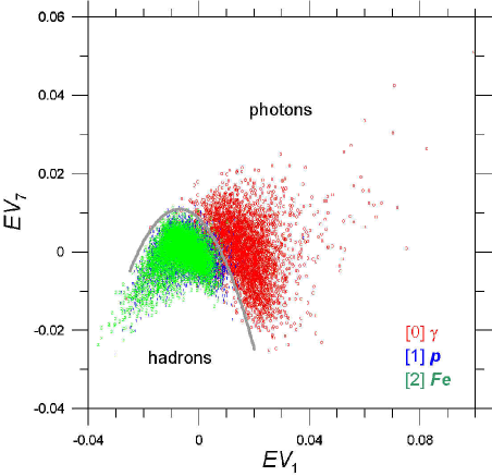
The best separation between nuclei and photons is obtained for the projection onto the plane defined by the first and seventh eigenvectors (see figure 1). The thick line, $EV_{7}=-48.89\times(EV_{1}+0.007)^{2}+0.011$, leaves only 0.8% of the nuclei in the region of photons and 12% of the photons in the region corresponding to nuclei. Therefore, the probability of misidentifying a photon is $2.7$% and the probability misidentifying a nuclei is $3.8$%.

Figure 1: PCA results on the illustrative parameter space. The best separation between nuclei and photons is obtained for the projection on the plane defined by the first and seventh eigenvectors. The thick line misclassifies $3.8$% of the nuclei as photons and $2.7$% of the photons as nuclei.

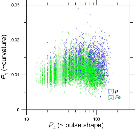
Once the photons have been separated, the same process can be applied to nuclei alone. However, as was stated before, this is a much more complicated problem as shown in figure 2. The optimization of of a diagnostic method in this case is still ongoing work.

Figure 2: Projection onto the $P_{1}$–$P_{4}$ plane of the sample points, once the photon events have been extracted, showing the difficulty involved in the separation of light and heavy nuclei.

3 Neural Network approach for p-Fe separation

3.1 QGSJet hadronic interaction model

An alternative approach for hadronic primary separation can be obtained by applying neural network technics to the problem.

An artificial neural network consists of a set of simple processing units which communicate by sending signals to each other over a large number of weighted connections. In general terms, neurons are structured in an array of hidden layers bounded by input and output slabs. Each unit receives inputs from neighbors or external sources and computes an output, $y_{k}$, which is propagated to other units:

$$y_{k}=F_{k}\left(\Sigma_{j}w_{jk}\times y_{j}+b_{k}\right)$$ (7)

where the sum extends over all the units $j$ effectively connected to $k$, $y_{j}$ is the input to unit $k$ coming from unit $j$, $w_{jk}$ is the corresponding weight for that connection and $b_{k}$ is a bias or offset term. $F_{k}$ is the transfer function, usually a nondecreasing function of the total input. Weights are the result of a training process in which known input-output pairs are fed to the network.

As an example of this powerful method, in figure 3 we show the results for a feed forward network, i.e., data flows exclusively from input to output – no feedback present (Rumelhart et al., 1986; Hagan et al., 1996; Kros̈e and van der Smagt, 1996), constituted by four layers of neurons with 3, 20, 3 and 1 neurons respectively, with tan-sigmoid (hidden) and log-sigmoid (output) transfer functions. The network was trained using the resilient backpropagation training algorithm in order to overcome problems arising from the small derivative of the sigmoid function far from the origin.

The input parameters used, based on direct observables and reconstructed magnitudes from the surface array detector, are:

$$P_{1}=\frac{1}{N_{stat}}\times\Sigma_{i=1}^{N_{stat}}N_{vem,i}\left(\frac{r_{0,i}}{1000m}\right)^{3}$$ (8)

$$P_{2}=\frac{1}{N_{stat}}\times\Sigma_{i=1}^{N_{stat}}\left(T_{0,i}-T_{sp,i}\right)\left(\frac{r_{0,i}}{1000m}\right)^{-2}$$ (9)

$$P_{3}=\frac{1}{N_{stat}}\times\Sigma_{i=1}^{N_{stat}}\left(T_{10,i}-T_{0,i}\right)\left(\frac{r_{0,i}}{1000m}\right)^{-1}$$ (10)

$$P_{4}=\frac{1}{N_{stat}}\times\Sigma_{i=1}^{N_{stat}}\left(T_{50,i}-T_{0,i}\right)\left(\frac{r_{0,i}}{1000m}\right)^{-1}$$ (11)

$$P_{5}=\frac{1}{N_{stat}}\times\Sigma_{i=1}^{N_{stat}}\left(T_{90,i}-T_{0,i}\right)\left(\frac{r_{0,i}}{1000m}\right)^{-1}$$ (12)

plus energy ($P_{6}$), zenith angle ($P_{7}$) and number of triggered stations ($P_{8}$); where $N_{stat}$ is the number of triggered stations, $T_{sp,i}$ is the arrival time of the shower plane to station $i$ and $r_{0,i}$ is the distance of station $i$ to the shower axis.

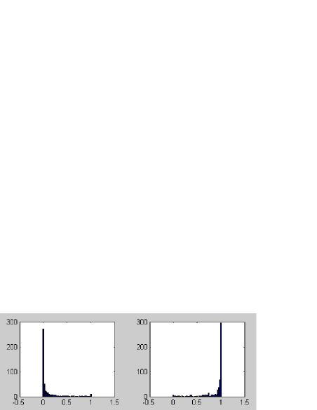
The network was trained to output 0 (1) for a proton (Fe) nucleus with a training set of 4000 events.

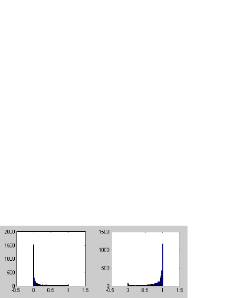
Figure 3 shows the result of applying the trained network to an independent control sample of 11600 events. Figures 3a,b show the classification results for protons and Fe respectively. It can clearly be seen that most of the control events ($80$% of protons and $\sim 87$% iron) are classified correctly.

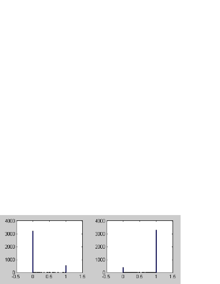
In order to assess the impact of using information coming from hybrid events, we performed an additional run including also $X_{max}$. The corresponding output is shown in figure 4. A noticeable improvement shows up clearly: $\sim 90$% of protons and $\sim 91$% iron are correctly classified. Furthermore, the number of ambiguous events with intermediate results between $0$ and $1$ diminishes noticeably producing a cleaner output.

3.2 Assessing hadronic interaction model dependence

The same network, trained under the assumption of the validity of the QGSJet model has been tested below at discriminating showers described by Sybill hadronic interactions. The results show once more the stability of the network solution despite the hadronic interaction model used.

Figure 3: Result of the application of a trained feed-forward network to an independent control sample of 11600 events triggered by protons and iron nuclei. The network was trained to output a value of zero (one) for a proton (iron) primary. Tails, therefore, correspond to misclassified events. Only surface array information was included.

Figure 4: Same as figure 3, but now hybrid events were considered (basically through the inclusion of X_max. A much clearer separation is obtained, despite some events are still misclassified.

Figure 5: The same neural network of figure 3, trained with EAS simulations based on the QGSJet hadronic interaction model is used to discriminate events described by Sybill hadronic interactions.