Mutual Constraints Between Reionization Models and Parameter Extraction From Cosmic Microwave Background Data

Abstract

Spectroscopic studies of high-redshift objects and increasingly precise data on the cosmic microwave background (CMB) are beginning to independently place strong complementary bounds on the epoch of hydrogen reionization. Parameter estimation from current CMB data continues, however, to be subject to several degeneracies. Here, we focus on those degeneracies in CMB parameter forecasts related to the optical depth to reionization. We extend earlier work on the mutual constraints that such analyses of CMB data and a reionization model may place on each other to a more general parameter set, and to the case of data anticipated from the $MAP$ satellite. We focus in particular on a semi-analytic model of reionization by the first stars, although the methods here are easily extended to other reionization scenarios. A reionization model can provide useful complementary information for cosmological parameter extraction from the CMB, particularly for the degeneracies between the optical depth and either of the amplitude and index of the primordial scalar power spectrum, which are still present in the most recent data. Alternatively, by using a reionization model, known limits on astrophysical quantities can reduce the forecasted errors on cosmological parameters. Forthcoming CMB data also have the potential to constrain the sites of early star formation, as well as the fraction of baryons that participate in it, if reionization were caused by stellar activity at high redshifts. Finally, we examine the implications of an independent, e.g., spectroscopic, determination of the epoch of reionization for the determination of cosmological parameters from the CMB. This has the potential to significantly strengthen limits from the CMB on parameters such as the index of the power spectrum, while having the considerable advantage of being free of the choice of the reionization model.

1 Introduction

The rapid progress in detector technology has led to the successful operation of many ground- and balloon-based experiments in the last few years for measuring the anisotropies in the CMB. Analyses of the recent data from experiments such as Boomerang (de Bernardis et al., 2002), MAXIMA-1 (Stompor et al., 2001), and DASI (Pryke et al., 2001) have confirmed the adiabatic cold dark matter (CDM) paradigm for describing the development of structure and the properties of the power spectrum of the CMB. They have also revealed that the universe is close to being spatially flat, and have begun to place tight constraints, in advance of satellite CMB experiments, on the cosmological parameters that describe our universe. Analyses of present data (see papers above, and those of, e.g., Tegmark et al. (2001) and Wang et al. (2001)) indicate, however, that strong degeneracies are still present in parameter extraction from the CMB, so that techniques to break these degeneracies continue to be valuable at present. Many of these degeneracies had been anticipated on theoretical grounds, and several methods to break them using observations of Type Ia SNe (Efstathiou et al., 1999), weak lensing (Hu, 2002), redshift surveys (Eisenstein et al., 1999; Wang et al., 1999; Popa et al., 2001), or combinations of these (Efstathiou & Bond, 1999) have been proposed. Ongoing and future CMB observations should provide markedly improved constraints on degenerate parameters through the detection of polarization in the CMB at large angular scales (Staggs & Church, 2001), and through dramatically increased sky coverage in the case of satellite experiments such as $MAP$ or $Planck$. The latter is especially important for overcoming cosmic variance for CMB multipoles, $l\lesssim$ 100. Current CMB data on the temperature anisotropy at degree and sub-degree scales provide an upper limit of about 0.3 for the optical depth to reionization, which may be translated to a model-dependent constraint on the redshift of hydrogen reionization, $z_{\rm reion}$ $\lesssim$ 25 (Wang et al., 2001).

Spectroscopic studies of high-$z$ quasars and galaxies blueward of Ly$\alpha$ have revealed the lack of a H I Gunn-Peterson (GP) trough, implying that the intergalactic medium (IGM) is highly ionized up to $z\sim 6$ (Fan et al., 2000; Dey et al., 1998; Hu et al., 1999). Recently, Djorgovski et al. (2001) presented observations of quasars at $z\gtrsim 5.2$ indicating a steady increase in the opacity of the Ly$\alpha$ forest for $z\sim$ 5.2–5.7, while Becker et al. (2001) presented a detection of the GP trough in the spectrum of the highest-redshift quasar known to date at $z\sim 6.3$ (Fan et al., 2001). Together, these data may be an indication of the epoch of H I reionization occurring not far beyond $z\sim 6$. As these authors have taken care to note, the detection of the GP trough in a single line-of-sight is not definitive evidence of $z_{\rm reion}\sim 6$; it may, however, be probing the end of the gradual process of inhomogeneous reionization coinciding with the disappearance of the last neutral regions in the high-$z$ IGM. This would be consistent with the lower end of the range of redshifts, $z\sim$ 6–20, predicted by theoretical models for H I reionization, either semi-analytic (Tegmark et al., 1994; Giroux & Shapiro, 1996; Haiman & Loeb, 1997; Valageas & Silk, 1999; Madau et al., 1999; Miralda-Escudé et al., 2000) or based on numerical simulations (Cen & Ostriker, 1993; Gnedin, 2000; Ciardi et al., 2000; Benson et al., 2001). Recent reviews of reionization may be found in Shapiro (2001), and Loeb & Barkana (2001).

The reionization of the IGM subsequent to recombination at $z\sim$ 1000 is thought to have been caused by increasing numbers of the first luminous sources. Although a variety of astrophysical objects or processes could have reionized the IGM, most of these group into stellar-related or QSO-related models, or equivalently, into sources with soft (star-like) or hard (QSO-like) ionizing spectra. Of these models, photoionization by stars and “mini-quasars” are at present the leading scenarios (Haiman & Knox, 1999; Loeb & Barkana, 2001), with the large majority of currently accepted reionization models involving stellar-type radiation for the following observationally motivated reasons. First, the space density of the large, optically bright QSO population appears to decrease after a peak at $z\sim$ 3. This has been confirmed by optical observations up to $z\sim$ 6.3 (Fan et al., 2001), and corroborated by radio surveys (Shaver et al., 1999) which should not suffer from the effects of dust obscuration. QSOs may however still be relevant to reionization, if they are powered by massive black holes that are postulated to form as a fixed universal fraction of the mass of collapsing halos at all redshifts (Haiman & Loeb, 1998; Valageas & Silk, 1999). This leads to a large population of faint QSOs (mini-quasars) in small halos at $z\gtrsim 6$ that are currently undetected. The observed turnover in the QSO space density at $z\gtrsim 3$ would then be true only for the brightest QSOs; this population, however, appears unlikely to cause H I reionization, either through their UV photons (Giroux & Shapiro (1996), and references therein; Fan et al. (2001)) or through the associated X-rays (Venkatesan et al., 2001). Second, if QSOs (mini- or otherwise) reionized the universe, we would expect the H I and He II reionization epochs to be coeval, given that QSOs are copious producers of H I and He II ionizing photons. The current data indicate that this does not occur, with He II reionization occurring at $z\sim$ 3 (Kriss et al., 2001), and that of H I reionization before $z\sim 6$. Thus the delayed reionization of He II relative to that of H I would seem to imply a metagalactic ionizing background dominated by a soft spectrum.

One might counter these two reasons with the argument that stars and quasars have similar effective ionizing power, which has been made frequently, most recently by Barkana (2002), and which goes as follows. The average efficiency with which the baryons in a high-$z$ halo form black holes that could power mini-QSOs is likely less than that for star formation. However, this is balanced by the higher escape fraction of ionizing radiation from mini-QSOs, given their inherently harder spectrum, leading to roughly the same overall output of IGM-ionizing photons per baryon in luminous objects. We note here that such arguments are limited by their not considering the detailed source spectrum which directly influences the growth of H II and He III regions, so that the observed delay in the reionization epochs of H I and He II remains unresolved quantitatively. Lastly, stars can account for the ubiquitous trace metallicity of about 0.003 of solar values seen in the low-density Ly$\alpha$ forest clouds up to $z\sim$ 4 (Venkatesan (2000), and references therein). A simple calculation shows that this detected metallicity implies a minimum (on average) of ten stellar ionizing photons per baryon having been generated in the past. This again implies that the first stars must play some role in reionization.

In summary, while the nature of the reionizing sources are at present unknown, the data suggest that their spectral properties resemble those of stars rather than quasars, and that radiation from the first stars is likely to have played a significant, if not the dominant, role in H I reionization. Therefore, in this work we will focus on a stellar origin for the reionizing spectrum, although we emphasize that one cannot at present rule out the possibility of alternate sources or a combination of high-$z$ source populations with individually varying spectral hardness that cause reionization. We refer the reader to Giroux & Shapiro (1996) for an excellent discussion on the relative roles of reionizing sources whose spectra are star-like, QSO-like and of intermediate spectral hardness. From this point onwards, reionization is always meant to refer to that of H I, rather than He II.

In this paper, we focus on those degeneracies in CMB parameter forecasts that involve the optical depth to reionization, $\tau$, based on methods developed in a previous work (Venkatesan (2000); henceforth Paper I) that examined the valuable complementary information provided by a reionization model. Typically, in CMB parameter extraction, the universe is assumed to reionize abruptly, leading to discretized values of $\tau$ in the multi-dimensional grid of models being tested in likelihood analyses of the data. This does not utilize, however, the strong sensitivity of $z_{\rm reion}$, and hence $\tau$, to specific parameters such as the spectral index of the primordial scalar power spectrum. As we noted in Paper I, $\tau$ is unique by definition amongst the set of standard cosmological parameters extracted from CMB data, being the only quantity which is not determined purely by the physics prior to the first few minutes after the Big Bang. Thus, it can potentially provide information on post-recombination astrophysical processes, if the other (cosmological) parameters which affect $\tau$ are well-constrained. We extend Paper I here to a larger parameter set in a $\Lambda$CDM cosmology; in the spirit of timeliness, we specifically consider the constraints anticipated from the data from the recently launched $MAP$ satellite, and we also include in our analysis the implications of an independent, e.g., spectroscopic, determination of $z_{\rm reion}$. Other improvements are detailed in the next section.

The plan of this paper is as follows. In §2, we review the reionization model that we consider and the formalism related to CMB parameter estimation. In §3, we present our results on the projected parameter yield from $MAP$, and we detail how a reionization model may improve constraints on cosmological parameters determined from the CMB, and vice versa. In §4, we discuss the implications of the secondary anisotropies generated in the CMB during reionization for the analysis in this work, and summarize the observations that are likely to best constrain the various aspects of reionization in the future. We conclude in §5.

2 Overview of the Reionization Model and CMB Analysis

The analysis in this paper essentially follows the methods developed in Paper I, which is extended here for a $\Lambda$CDM model; the points of departure and improvements here are described below.

We assume that stars are responsible for reionization (for the reasons presented in §1), and use the semi-analytic stellar reionization model developed by Haiman & Loeb (1997), with the modifications described in Paper I. We take the primordial matter power spectrum of density fluctuations to be, $P(k)\propto k^{n}$ $T^{2}(k)$, where $n$ is the index of the scalar power spectrum, and the matter transfer function $T(k)$ is taken from Eisenstein & Hu (1998). We normalize $P(k)$ to the present-day rms density contrast over spheres of radius 8 $h^{-1}$ Mpc, $\sigma_{8}$.

We track the fraction of all baryons in star-forming halos, $F_{\rm B}$, by the Press-Schechter formalism, allowing star formation only in halos of virial temperature $\gtrsim$ 10⁴ K, corresponding to the mass threshold for the onset of hydrogen line cooling. The details concerning the adopted stellar spectrum of ionizing photons and the solution for the growth of ionization regions around individual halos may be found in Paper I. We define reionization as the epoch of overlap of individual H II regions, i.e., when the volume filling factor of ionized hydrogen, $F_{\rm H\,II}$ = 1. We include the effects of inhomogeneity in the IGM through a clumping factor, $c_{L}$, rather than assuming a smooth IGM as in Paper I. We define $c_{L}$ to be the space-averaged clumping factor of ionized hydrogen, $c_{L}$ $\equiv$ $<$ $n_{p}^{2}$ $>$/$<n_{p}>^{2}$ (Shapiro & Giroux, 1987; Madau et al., 1999), which is equivalent to $<n_{e}^{2}>$/$<$ $n_{e}$$>^{2}$ in this work as the sources of photoionization do not generate any helium-ionizing photons. The optical depth to reionization from electron scattering is then given by:

$$\tau\simeq 0.057\;\Omega_{\rm b}h\;\int_{0}^{z_{\rm reion}}dz\;\frac{(1+z)^{2}\;[1-f_{\star}F_{\rm B}(z)]\;F_{\rm H\,II}(z)}{\sqrt{\Omega_{\Lambda}+(1+z)^{2}(1-\Omega_{\Lambda}+\Omega_{\rm m}z)}}.$$ (1)

The optical depth to reionization depends upon a number of parameters as, $\tau$ = $f$($\sigma_{8}$, $\Omega_{b}$, $h$, $n$, $\Omega_{\Lambda}$, $\Omega_{\rm M}$, $f_{\star}$, $f_{esc}$), where $f_{\star}$ is the fraction of baryons in each galaxy halo forming stars, $f_{esc}$ is the escape fraction of H I ionizing photons from individual halos, $h$ is the Hubble constant in units of 100 km s^-1 Mpc^-1, and the other symbols have their usual meanings. We fix $\Omega_{\rm K}$ = 1 - $\Omega_{\rm M}$ - $\Omega_{\Lambda}$. We also set $f_{esc}$ = 0.1 (Dove et al., 2000; Leitherer et al., 1995), so that it is no longer a free parameter as it was in Paper I, for the following reasons. First, the mass threshold scale for the Press-Schechter evolution of halos in our model corresponds to massive halos of virial temperature $\gtrsim 10^{4}$ K. The baryons in such halos are likely to be collisionally ionized, at least partly, so that $f_{esc}$ $\ll$ 1 is unlikely. The values of $f_{esc}$ in low-mass systems (masses $\lesssim$ $10^{7}M_{\odot}$) at high redshift have been studied by Ricotti & Shull (2000). Second, as shown in Haiman & Loeb (1997) and Paper I (see in particular Table 1 and the associated discussion), $\tau$ is not very sensitive to the chosen values of $f_{esc}$, once they exceed a few percent. Third, limits on $\tau$ from the CMB, being a single number, can be translated to a constraint on any one non-cosmological parameter that determines $\tau$; recall, for example, that in Paper I, both $f_{\star}$ and $f_{esc}$ could not be constrained simultaneously from the CMB. Hence we choose to retain $f_{\star}$ as the primary astrophysical input parameter, as $\tau$ is most sensitive to it in our chosen reionization model.

To be complete, we note that observations of Lyman-continuum emission from Lyman-break galaxies at $z\sim$ 3.4 by Steidel et al. (2001) indicate values of $f_{esc}$ exceeding 0.5. Also, some simulations of reionization by stars often appear to require or imply similarly high values for $f_{esc}$ (Gnedin, 2000; Benson et al., 2002) in order to have $z_{\rm reion}$ exceed $\sim$ 7. The large derived value for $f_{esc}$ in the former case arises partly from the definition itself of $f_{esc}$; as Steidel et al. (2001) noted, their chosen observational procedure normalized the escape fraction of 900Å photons to that of 1500Å photons. Data from the local universe (Deharveng et al., 2001; Leitherer et al., 1995), especially of high-mass systems, generally do not support values of $f_{esc}$ exceeding about 10%.

Reionization affects the CMB through the Thomson scattering of CMB photons from free electrons in the IGM. This leads to an overall damping of the primary temperature and polarization anisotropies in the CMB, except at the largest angular scales (small $l$), and the generation of a new feature in the polarization power spectrum. The first effect can be distinguished from CMB anisotropies with slightly lower peak amplitudes (corresponding to a lower $\sigma_{8}$ in our model) only at the lowest $l$s, but cosmic variance obscures the difference at such scales. This is the origin of the amplitude–reionization degeneracy in the CMB temperature power spectrum. However, the reionized IGM creates a linear polarization signal which peaks at the horizon size at $z_{\rm reion}$, so that the amplitude and angular location of this new feature are comparatively direct probes of the values of $\tau$ and $z_{\rm reion}$ respectively (Zaldarriaga, 1997). A detection of polarization in the CMB at large angular scales can therefore constrain $\tau$ far more accurately than can temperature data alone, and has the potential to break the above degeneracy. In practice, it may prove difficult to measure, given that the polarization anisotropy is expected to be only at the $\sim$ 10% level relative to that in the CMB’s temperature, and that for late reionization the above feature has an extremely small amplitude (see next section). Additionally, foregrounds are likely to complicate the extraction of a polarization signal at low $l$. As we do not consider tensor contributions to the primordial matter power spectrum, polarization here refers to the E-channel type. Lastly, we do not explicitly consider the effects of any secondary anisotropies generated in the CMB during reionization, but we return to this topic in §4.

Parameter extraction from the CMB is based on the methods outlined in Paper I. For cases involving $\tau$ and a set of cosmological parameters, we follow the industry-tested Fisher matrix formalism in, e.g., Knox (1995), Jungman et al. (1996), Zaldarriaga et al. (1997), and Bond et al. (1997). If we expand the angular power spectrum of the CMB in terms of its multipole moments $C_{l}$, and assume Gaussian initial perturbations and that the $C_{l}$ are determined by a fiducial set of parameters describing the “true” universe, then we can quantify the behavior of the likelihood function of observing any set of $C_{l}$s near its maximum, given the fiducial parameter set, in terms of the Fisher information matrix, $F_{ij}$. If we further assume that the likelihood function has a Gaussian form near its maximum, the elements of $F_{ij}$ can be expressed as the product of pairs of derivatives of the $C_{l}$ with respect to the appropriate parameters. The Fisher matrix represents the best accuracy with which parameters in the chosen “true” model can be estimated from a CMB data set. The inverse of $F_{ij}$ is the covariance matrix between the parameters; the minimum 1 $\sigma$ error in a parameter $P_{i}$ is given by $\sqrt{(F^{-1})_{ii}}$.

The reionization model, as described above, yields $\tau$ = $\tau$($\sigma_{8}$, $\Omega_{b}$, $h$, $n$, $\Omega_{\Lambda}$, $\Omega_{\rm M}$, $f_{\star}$) = $\tau$($P_{\rm cosmo}$, $f_{\star}$), while the CMB data determines [$P_{\rm cosmo},\tau(P_{\rm cosmo},f_{\star})$]. We can therefore use a reionization model to relate and mutually constrain ($P_{\rm cosmo},f_{\star}$). In such cases, the derivatives of the CMB multipoles, $C_{l}$, that are used to construct the Fisher matrix become (Paper I):

$$\frac{\partial C_{l}}{\partial P_{\rm cosmo}}=\;\left.\frac{\partial C_{l}}{\partial P_{\rm cosmo}}\right|_{\tau}\;+\;\;\left.\frac{\partial C_{l}}{\partial\tau}\right|_{P_{\rm cosmo}}\frac{\partial\tau}{\partial P_{\rm cosmo}}$$ (2)

$$\frac{\partial C_{l}}{\partial f_{\star}}=\;\frac{\partial C_{l}}{\partial\tau}\frac{\partial\tau}{\partial f_{\star}}$$ (3)

Parameter estimation is performed using theoretical CMB power spectra generated by CMBFAST [version 4.0; Seljak & Zaldarriaga (1996)]. This version of CMBFAST corrects a bug in previous versions related to some models with non-zero values of $\tau$, and includes an improved treatment of recombination based on the work of Seager et al. (2000). Although the primordial power spectrum in the reionization model and the CMB may be normalized to $\sigma_{8}$ or the COBE normalization (both of which themselves depend on a number of cosmological parameters), we choose the former option for the following reasons. First, there is a large difference between the physical scales probed by COBE on which linear physics operates, and those that are relevant for reionization and the formation of the first luminous objects (tens of kpc and below). In order to bridge this gap between mass fluctuations in the linear and highly nonlinear regimes, it is more consistent to use a parameter such as $\sigma_{8}$, which probes the amplitude of the fluctuations in the power spectrum today at intermediate scales. This choice is particularly important in a work such as this, where constraints from a model that describes the activity of the reionizing sources are combined with those from the CMB. Second, $\sigma_{8}$, like the COBE normalization, is a well-defined observational parameter that is currently measured to within 10% error. As reionization is sensitive, however, to the amount of power on small scales, the uncertainty in the value of $\sigma_{8}$ translates to a lower relative error in the amount of small-scale power than does the same uncertainty in the value of the COBE normalization, particularly when a parameter such as $n$ is varied. Thus, normalizing to $\sigma_{8}$ rather than to COBE reduces any purely normalization-related effects of small variations in $n$ on the amount of power available on small scales, due to the shorter lever arm between the physical scales associated with $\sigma_{8}$ and reionization. This is an important consideration for this paper, one of whose results demonstrate the sensitivity of $z_{\rm reion}$ to $n$.

In this work, we focus specifically on the constraints anticipated from the data from the $MAP$ satellite. We include the effects of instrumental noise, rather than assuming cosmic variance limited data as in Paper I. We take experimental specifications and the method of constructing $F_{ij}$ from Eisenstein et al. (1999), and assume that foregrounds can be effectively subtracted from $MAP$ data (Tegmark et al., 2000). In all the figures below, the error ellipses, where displayed, represent 68% joint confidence regions.

3 Results

We now discuss the constraints that a stellar reionization model and CMB parameter forecasts may place on each other. We define our standard model (SM) as described by the 7-parameter set, [$\sigma_{8}$, $\Omega_{b}$, $h$, $n$, $\Omega_{\Lambda}$, $\Omega_{\rm M}$, $\tau$/$f_{\star}$] = [1.0, 0.04, 0.7, 1.0, 0.7, 0.3, 0.048/0.05]. As mentioned earlier, $\Omega_{\rm K}$ is fixed to be [1 - $\Omega_{\rm M}$ - $\Omega_{\Lambda}$] in the parameter analyses below, and its value is zero only in the SM. We set the clumping factor $c_{L}$ = 30 (see, e.g., Madau et al. (1999), and references therein), which, together with our choice of $f_{esc}$ = 0.1 (§2), leads to $\tau\sim$ 0.048 for the SM, corresponding to a reionization epoch of $z_{\rm reion}=8$. The average ionization fraction of the IGM in the SM is $10^{-4}$, $10^{-3}$, 0.01, 0.1, and 1.0 at the respective redshifts of about 18, 15.6, 13.2, 10.6, and 8. This is consistent with the evolution of the volume-averaged hydrogen ionization fraction in numerical simulations of reionization with the same background cosmology as the SM here (see, e.g., Figure 10 of Gnedin 2000.)

Our choice of parameters for the SM, though well-motivated and in concordance with a variety of observations, is deliberately constructed to generate late reionization, given the recent observational claim of detecting the last stages of reionization at $z\sim 6.3$. The semi-analytic treatment here defines reionization as the overlap of H II regions, and corresponds to the component of the IGM that dominates the ionization by volume filling factor at high redshift. By this definition, reionization somewhat precedes the disappearance of the GP trough in the IGM (Haiman & Loeb, 1999), which represents the ionization of any remaining H I in highly overdense or clumped portions of the IGM, or in individual H II regions. Note also that the power of the CMB to constrain cosmological parameters is often better demonstrated by considering parameter combinations such as $\Omega_{b}h^{2}$ and $\Omega_{\rm M}h^{2}$ rather than individual ones. We have chosen our parameter as displayed above in order to make an apples-to-apples comparison between the dependency of the CMB power spectra and the reionization model on these individual cosmological parameters. Furthermore, our intent in this work is to show that a reionization model can tighten constraints from the CMB on, e.g., $n$, but not on parameter combinations such as $\Omega_{b}h^{2}$ and $\Omega_{\rm M}h^{2}$ because these will be very well-determined by CMB data alone.

As a reference, we show in Figure 1 the angular temperature and polarization power spectra of the CMB for the SM. As we noted earlier, the main effect of the reionization of the IGM is an overall damping of the primary CMB temperature and polarization anisotropies. It also generates a new feature in the CMB polarization spectrum corresponding to the horizon size associated with $z_{\rm reion}$; for the late reionization in our SM, this corresponds to the polarization bump at $l\lesssim 5$. The signal associated with this unique probe of reionization has an extremely small value, being less than the temperature anisotropy by over two orders of magnitude at these scales.

Figure 1: Theoretical temperature and $E$-channel polarization angular power spectra of the CMB in units of $\mu$K for this work’s standard model (SM), shown by the solid line: $\sigma_{8}$ = 1.0, $\Omega_{b}$ = 0.04, $h$ = 0.7, $n$ = 1.0, $\Omega_{\Lambda}$ = 0.7, $\Omega_{\rm M}$ = 0.3, $\tau$ = 0.048. Dashed lines display the power spectra for the same choice of cosmological parameters with $\tau$ = 0; the difference is noticeable only for $l\lesssim 20$.

3.1 Using a Reionization Model to Improve Constraints from the CMB

Using the techniques in §2, we can use a reionization model to constrain cosmological parameters beyond the limits obtained from CMB data alone, through $\tau$ or $f_{\star}$. Let us first focus on the former case. Certain combinations of parameters are well known to be degenerate in CMB parameter extraction, such as $\tau$–$\sigma_{8}^{2}$ and $\tau$–$n$ (see, e.g., the recent analyses by the DASI, MAXIMA-1 and Boomerang collaborations). A reionization model can provide complementary information, as $\tau$ is itself a function of cosmological parameters, and break such degeneracies. We display this in Figures 2 and 3, for the above combinations of degenerate parameters, where we marginalize only over the respective two-dimensional spaces and keep all the other parameters fixed at their SM values. The dark outer and light inner ellipses correspond to the 1 $\sigma$ constraint from $MAP$’s temperature (T), and temperature plus polarization (T+P) data. The thin solid line represents the functional dependence of $\tau$ on $n$ or $\sigma_{8}^{2}$ from the reionization model for $f_{\star}$ = 0.05, and the dashed lines represent the possible range for $\tau$, given the uncertainty in the value of $f_{\star}$. This possible range for $f_{\star}$ of $\sim$ 0.01–0.15 comes from the results of numerical simulations and from arguments of avoiding excessive metal pollution of the IGM at late redshifts (Paper I, and references therein); it represents the astrophysical uncertainty in our chosen reionization model, given the choice to set those $P_{\rm cosmo}$ other than $n$ or $\sigma_{8}^{2}$ to their values in the SM. Figures 2 and 3 show that the reionization model can be valuable in breaking degeneracies in CMB parameter analyses, even when given the range in the potential values of $f_{\star}$.

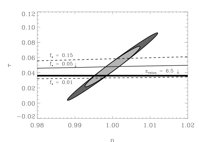
Figure 2: Constraints from the reionization model and projected data from $MAP$ in the $\tau$–$n$ plane, after 2-D marginalization over the [$\tau$, $n$] space with all other parameters fixed at their SM values. The thin solid line displays $\tau$ as a function of $n$ from the reionization model with $f_{\star}=0.05$, and the dashed lines represent the astrophysical uncertainty in $\tau$, given the permitted range of 0.01–0.15 in the value of $f_{\star}$. The dark outer and light inner ellipses correspond to the 1 $\sigma$ joint confidence regions from $MAP$’s temperature, and temperature plus polarization data. Note the strong dependence of $z_{\rm reion}$, and hence $\tau$, on $n$ through the reionization model (thin solid line): for $n$ = 0.98–1.02, $z_{\rm reion}$ $\sim$ 7.75–8.2. The thick solid line represents the constraint from a hypothetical independent measurement of $z_{\rm reion}$ = 6.5.

Figure 3: Constraints from the reionization model and projected data from $MAP$ in the $\tau$–$\sigma_{8}^{2}$ plane, after 2-D marginalization over the [$\tau$, $\sigma_{8}^{2}$] space with all other parameters fixed at their SM values. Plot legend is the same as in Figure 2.

The main source of the dependence of $\tau$ on $n$ and $\sigma_{8}^{2}$ is $z_{\rm reion}$, and to a lesser extent, the term $f_{\star}F_{\rm B}$ in eqn. 1, which is never more than a 2% effect in the value of $\tau$ for the SM. Ideally, we would like to characterize $\tau$ as a function of $P_{\rm cosmo}$, in order to eliminate its dependence on the astrophysical details of reionization. If we neglect the term $f_{\star}F_{\rm B}$, eqn. 1 is considerably simplified as $F_{\rm H\,II}$ = 1.0 along the line-of-sight from the present ($z=0$) to $z=z_{\rm reion}$. The problem now reduces to parametrizing $z_{\rm reion}$ in terms of $P_{\rm cosmo}$ alone; in reality, however, $z_{\rm reion}$ is a non-unique function of various cosmological parameters as well as the specific (astrophysical) reionization scenario. The analysis of Griffiths et al. (1999), while having the advantage of being fitted to the available data at the time, encountered the same problem of being unable to uniquely relate $z_{\rm reion}$ to the cosmological parameters that they considered ($h$, $n$, $\Omega_{0}$); the fit provided by them for $\tau$ as a function of these three parameters was purely empirical but not based on any model of the reionizing sources. Thus, the only way to utilize the valuable sensitivity of $\tau$ to $n$ and $\sigma_{8}^{2}$ is via a reionization model. The importance of retaining the information contained in $z_{\rm reion}$, particularly for the lower bound on $n$, was noted in Covi & Lyth (2001), where they pointed out that the choice to leave $z_{\rm reion}$ as a free parameter, e.g., in the analysis of Tegmark et al. (2001), could lead to an artificially lowered value of $n$ from CMB data.

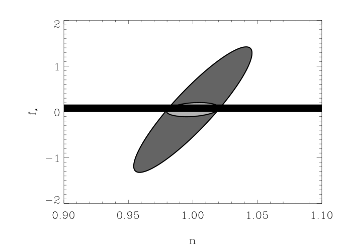
Figure 4: Constraints from the projected data from $MAP$ in the $f_{\star}$–$n$ plane after full 7-D marginalization over the [$f_{\star}$, $P_{\rm cosmo}$] space. The dark outer and light inner ellipses correspond to the 1 $\sigma$ joint confidence regions from $MAP$’s temperature, and temperature plus polarization data. Solid horizontal band represents the entire allowed astrophysical range of 0.01–0.15 for $f_{\star}$.

What if, however, there were an independent limit on $z_{\rm reion}$? One possible method, which involves relating $z_{\rm reion}$ directly to the fraction of baryons in star-forming halos, $F_{\rm B}$, has been explored by Covi & Lyth (2001) and Tegmark et al. (1994). Subject to theoretical uncertainties, this is well motivated, as regardless of the details of the nature and the sources of reionization, one requires in the end a certain number of IGM-ionizing photons per baryon in collapsed structures. Another possibility, which may shortly be upgraded to reality, would be a spectroscopic detection of $z_{\rm reion}$ through the GP effect in the absorption-line spectra of the highest-$z$ sources (see §1). The great advantage of this second kind of independent determination of $z_{\rm reion}$ is that one may safely bid farewell to the pesky details of “gastrophysics” (Bond, 1995) in parametrizing $\tau$ for CMB parameter extraction! If we drop the term $f_{\star}F_{\rm B}$ in eqn. 1, we can now relate $\tau$ to the $P_{\rm cosmo}$ other than $n$ and $\sigma_{8}^{2}$. This leads to a unique value of $\tau$ in the 2-D space of Figures 2 and 3, which is depicted as the thick solid line for a hypothetical measured value of 6.5 for $z_{\rm reion}$. Such a detection can be useful in breaking parameter degeneracies and improving constraints from the CMB without invoking a specific reionization model. Note that a detection of $z_{\rm reion}$ cannot be translated to a unique prior on $\tau$ for multi-parameter marginalization, as the latter is also determined by cosmological parameters such as $\Omega_{\Lambda}$, $\Omega_{b}$, etc. Thus, an independent determination of $z_{\rm reion}$ is best utilized in the 2-D spaces of parameter combinations that are degenerate with $\tau$, such as the examples in Figures 2 and 3.

We now move on to the second case defined at the beginning of this section, where one may translate astrophysical limits to constrain cosmology. We marginalize over the 7-D space of [$f_{\star}$, $P_{\rm cosmo}$] rather than [$\tau$, $P_{\rm cosmo}$], by using the reionization model to relate them via $\tau$ (eqns. 2 and 3). We can then apply independent limits on $f_{\star}$ (0.01–0.15) to further constrain $P_{\rm cosmo}$. Figure 4 displays one such case in the $f_{\star}$–$n$ subspace for the projected constraints from $MAP$’s T and T+P data. Despite the error ellipses being lower bounds to those that $MAP$ will provide (given our assumption of successful foreground removal), the entire astrophysical permitted band for $f_{\star}$ can still reduce the 1-$\sigma$ error for $n$. Although one may propose alternate ranges for $f_{\star}$, we anticipate that the main point here– that known constraints on $f_{\star}$ have the power to strengthen limits from the CMB on $P_{\rm cosmo}$– will still hold true.

In summary, using a reionization model can break degeneracies in CMB parameter estimation related to $\tau$, and improve the errors from $MAP$ data on $n$ and $\sigma_{8}^{2}$ by factors of at least 3–6 and 3–10 respectively for the case of $f_{\star}=0.05$. Alternatively, known astrophysical limits on $f_{\star}$ can reduce the errors on $P_{\rm cosmo}$ from $MAP$, e.g., by up to a factor of 2 for $n$ from $MAP$ temperature data. The strongest cross-constraint in the near future may be provided by an independent measurement of $z_{\rm reion}$, which could reduce the 1 $\sigma$ errors on parameters that are degenerate with $\tau$, such as $n$ or $\sigma_{8}^{2}$, by factors of 3–10. The non-trivial advantage of this last method is that it is independent of one’s choice of reionization model.

3.2 Using CMB Data to Constrain a Reionization Model

Given the framework of this paper, there are at least two ways that forthcoming CMB data may be used to constrain aspects of reionization. First, we can use a reionization model to extract [$f_{\star}$, $P_{\rm cosmo}$] rather than [$\tau$, $P_{\rm cosmo}$] from CMB data. Table 1 displays the 1 $\sigma$ errors from $MAP$ T and T+P data for full marginalization over the 6-D [$P_{\rm cosmo}$] and the 7-D [$\tau$, $P_{\rm cosmo}$] parameter spaces. Both the 6-D and 7-D cases assume 65% sky coverage and factor in the effects of instrumental noise for $MAP$. Including $\tau$ in the analysis significantly worsens error bars from $MAP$’s T-data, particularly for $\sigma_{8}^{2}$ and $n$; this can be expected from the degeneracies discussed above. Put another way, excluding $\tau$ or setting it to be zero can lead to deceptively small errors in parameters such as $\sigma_{8}^{2}$ and $n$.

Table 1: Projected 1 $\sigma$ errors from $MAP$ data

		Without $\tau$		With $\tau$		Ideal $MAP$
Parameter		T	T+P	T	T+P	T+P
$\tau$ [$f_{\star}$]				0.193 [0.904]	0.022 [0.102]	[0.011]
$\sigma_{8}^{2}$		0.048	0.047	0.079	0.047	0.026
$\Omega_{b}$		0.003	0.003	0.004	0.003	0.002
$h$		0.022	0.022	0.026	0.022	0.012
$n$		0.013	0.013	0.03	0.013	0.008
$\Omega_{\Lambda}$		0.018	0.018	0.022	0.018	0.008
$\Omega_{\rm M}$		0.019	0.018	0.019	0.018	0.01

Using the reionization model now to relate $f_{\star}$ and $P_{\rm cosmo}$ (eqns. 2 and 3), we see from Table 1 that $MAP$’s T and T+P data do not constrain $f_{\star}$ very strongly. If, however, $MAP$ can achieve being cosmic variance limited to $l\sim 500$ with 50% sky coverage, which we label as “Ideal $MAP$” in the table, it is possible with T+P data to determine $f_{\star}$ to significantly greater accuracy than its currently allowed range. Given that we have not factored in foreground contamination of the CMB polarization signal, which particularly degrades parameter extraction on the (large) scales at which reionization has a unique signature (Tegmark et al., 2000; Baccigalupi et al., 2001), our prediction of strong limits on $f_{\star}$ from the CMB may be somewhat optimistic.

A second possibility involves using a measurement of $\tau$, particularly through polarization in the CMB; current data place only rough upper limits of $\tau$ $\lesssim$ 0.3. A low net value of $\tau$ would imply that star formation cannot be widespread, or that it has to be fairly inefficient. The majority of the theoretical models to date imply that reionization takes place between $z\sim$ 8–20. In our SM, we allow star formation only in halos of virial temperature $\gtrsim$ 10⁴ K. If we replace this mass threshold scale in our Press-Schechter evolution with the Jeans mass scale at each redshift, then, for the SM cosmological parameters, we obtain $\tau\sim 0.078$ (0.11), and $z_{\rm reion}\sim 11.25$ (14.2) with (without) clumping. Thus, as an example, if $\tau$ were measured in the future to be $\lesssim$ 0.05, it would imply that early star formation has to be relatively rare, i.e., occurs in high-mass rather than in low-mass halos at high redshifts, or that it is relatively inefficient (values of $f_{\star}$ significantly less than in the SM). While this statement relies on our assumptions and adopted reionization model in this work, it is a potential constraint in the near future.

In summary, forthcoming CMB data may be able to constrain the fraction of baryons that participated in early star formation, and, more speculatively, the sites of such stellar activity as well, if reionization were caused by stars.

4 Discussion

In this work, we have focussed primarily on tightening constraints on cosmological parameters and on constraining aspects of the reionizing source population from CMB data by using either a semi-analytic reionization model for $\tau$ or an independent determination of $z_{\rm reion}$. For this purpose, we have considered only the first-order effects of reionization: the damping of the primary CMB anisotropies and the generation of a new polarization signal at large angular scales. This was motivated by the possibility of these signatures being detected imminently, and by the simplicity of parametrizing them. The reader may, however, wonder to what degree the results presented here depend on the adopted reionization model, and on the effects of inhomogeneous reionization and the secondary CMB anisotropies generated during reionization which were not considered here. We address these issues below; we also discuss which observations of the CMB and high-$z$ large scale structure have the potential to constrain not only $z_{\rm reion}$, but also the duration, inhomogeneity and physical processes related to reionization.

We have chosen stars as the principal reionizing source population for the observationally motivated reasons described in §1. We emphasize that other possibilities, such as a large high-$z$ population of mini-quasars that are as yet undetected, or a combination of stars, quasars and other sources cannot be ruled out at present. The methods in this paper are, however, easily extended to other reionization scenarios. Since the relevant quantity for reionization is the average ionizing efficiency of each baryon in luminous objects, the constraints in this paper involving $f_{\star}$ may be equivalently regarded as limits on the fraction of baryons in individual halos that formed objects with a star-like (soft) ionizing spectrum. The calculations in this paper can be applied equally well to sources with QSO-like (hard) ionizing spectra, including the case of metal-free stars, but such reionization models face the added consideration of accounting for the observed lag of the He II reionization epoch relative to that of H I.

Although we include the effects of IGM clumping in this paper, the development of luminous objects and the gradual overlap of H II regions are themselves characterized only in an average homogeneous sense. In reality, the first astrophysical sources of ionizing photons are likely to be located in very dense regions embedded in the large scale filamentary structure of matter, so that reionization is a highly nonlinear, inhomogeneous process. To probe the complex details of this so-called patchy reionization, one must turn to numerical simulations, which can follow the detailed radiative transfer and reveal the full 3D topology of reionization. Simulations are also very useful for quantifying the secondary anisotropies generated in the CMB during reionization, because they can perform the necessary characterization of the spatial variation of the ionization levels. Inhomogeneous reionization generates second-order temperature anisotropies in the CMB, with contributions from the spatially varying electron density and the bulk velocity field of the electrons. The first effect can be caused by variations in the baryon density (Ostriker & Vishniac, 1986) or in the ionization fraction (patchy reionization), the latter depending on the typical size of H II regions around individual sources and on the spatial correlations of ionized gas.

The amplitude of these second-order features can in principle constrain $z_{\rm reion}$, as well as the nature and sites of the reionizing sources through the angular scale on which they generate a secondary signal in the CMB. Detailed studies of these effects (see, e.g., Gnedin & Jaffe (2001), and references therein, Benson et al. (2001)) indicate, however, that the secondary anisotropy spectrum is dominated by the thermal Sunyaev–Zeldovich effect from low-$z$ clusters of galaxies at CMB multipoles $l\sim$ 1000–$10^{5}$, with the kinetic Sunyaev–Zeldovich effect taking over at $l\gtrsim 10^{5}$. The signal from the patchiness of reionization (the spatial variation of the ionization fraction) appears to be subdominant at all angular scales to the two effects above, if the ionizing sources are clustered on the scales that are typical of stellar and mini-QSO models. The signature of patchy reionization in the CMB may be detected, however, if reionization were caused by spatially rare, bright objects having comparatively large H II regions, although this will still occur at extremely large $l$, and the sources in such a case cannot be large bright QSOs from the discussion in §1. The geometry of reionization also partly determines the amplitude of such secondary anisotropies; the signal is relatively low if the low-density IGM regions are ionized first, which is likely. For the signal from patchy reionization to be dominant, $z_{\rm reion}$ would have to exceed its current upper bound of $\sim$ 30 from CMB data. Lastly, the dominant contributions to secondary CMB anisotropies from reionization come from the epochs just preceding $z_{\rm reion}$, and from the correlations between high-density regions, which trace the underlying matter density field rather than the varying ionization of the IGM itself (Valageas et al., 2001).

Thus, as Gnedin & Jaffe (2001) state, the prospects for describing the details of reionization, such as its inhomogeneity and duration, through secondary anisotropy signatures at sub-degree scales in the CMB are not very encouraging, as they are not likely to be within the detection capabilities of the next decade of CMB experiments. Although numerical simulations, given their computational expense, are not a practical method of quantifying the role of patchy reionization in the likelihood analyses in CMB parameter estimation, their findings indicate that second-order effects from reionization are not likely to contaminate parameter extraction from CMB data in the near future. This justifies our approach in this work where we have concentrated on the first-order effects of reionization on the CMB; most of the information on $\tau$ comes from a large-scale polarization signal, which is not complicated by the inhomogeneity of reionization manifesting in the CMB at much smaller angular scales.

The semi-analytic reionization model used in this paper is formulated through a generally accepted prescription with simple physics, thereby reducing a large body of possible input parameters to the essential ones. The advantage of using a model for $\tau$ is that we have a simple well-motivated model that does not introduce additional parameters (unlike Paper I), and that relates the CMB data to the most important quantity driving reionization. In the case of the reionization model considered here, this quantity happens to be $f_{\star}$, but it could equivalently be $f_{esc}$ or other parameters that describe the sources of reionization. We have also demonstrated how future CMB data may be able to constrain the sites of early star formation, as well as the fraction of baryons that participated in it, assuming a stellar reionization scenario. Lastly, a reionization model allows us to strongly constrain parameters such as $n$ with CMB data, as $z_{\rm reion}$ is very sensitive to the amount of small-scale power.

The drawback of some of the results presented here is the use of model-dependent means to break degeneracies or tighten constraints on cosmological parameters in CMB data analyses. It would be more preferable to combine data sets to accomplish this, which numerous papers have explored using, e.g., weak lensing data or large scale structure data from the IRAS PSCz Survey, the Sloan Digital Sky Survey (SDSS), the 2dF Survey, etc. (§1). Although such data of the local universe will not directly constrain $\tau$, they will add information that is complementary to the CMB on parameters such as $n$ and the power spectrum normalization, thereby helping to break degeneracies between these parameters and $\tau$ in CMB parameter estimation. Hence, the use of a reionization model may not be necessary. One may then ask what sort of data related to reionization will prove valuable for CMB analyses. We have taken a first step in this work towards answering this question by demonstrating the power of an independent determination of the reionization epoch (Figures 2 and 3) to break parameter degeneracies in the CMB, and to sharply reduce the error on parameters such as $n$.

The most promising data avenue to probe the sources, duration, and inhomogenous aspects of reionization will likely be high-resolution spectroscopic studies with high signal-to-noise of bright quasars and starforming galaxies at $z\gtrsim$ 6. The current evidence for a complete H I GP trough, and hence $z_{\rm reion}$, comes from the spectrum of a single $z\sim$ 6.3 QSO. The acquisition of more data along many more lines of sight to sources at $z\sim$ 6–10 is required to adequately represent how the appearance and duration of the GP trough varies with redshift and different sightlines through the IGM. This will lead to an angular map on the sky of $z_{\rm reion}$ as a function of sightline, which will dramatically increase our power to quantify the spatial nonuniformity of the reionization process, the size distribution of ionized regions, the nature of the ionizing sources, and the physical conditions in an average region of the IGM during reionization (Barkana, 2002). Such observations are within the capabilities of the SDSS, which should detect about 20 bright quasars at $z\gtrsim$ 6 during the course of the survey (Becker et al., 2001), and are important targets in the planning of the Next Generation Space Telescope. Such data would also permit the direct extraction of $z_{\rm reion}$ from the portions of transmitted flux between the individual troughs from the Lyman series lines for sources that lie just beyond $z_{\rm reion}$ (Haiman & Loeb, 1999), although this could be complicated by intervening IGM clumpiness or damped Ly$\alpha$ systems. Such spectroscopic studies will be invaluable for characterizing the scale dependence of the high-$z$ IGM’s porosity in the epochs around $z_{\rm reion}$; the challenge will be to understand which of the cosmic variance in the data arises from the underlying mass distribution rather than the “gastrophysics” manifested through patchy ionization.

In addition to Ly$\alpha$ GP trough studies, Umemura et al. (2001) have suggested that the H$\alpha$ forest is a significantly more powerful probe of the ionization history of the universe at $z\gtrsim 5$. The H$\alpha$ line is more sensitive to small changes in the degree of ionization when the IGM neutral fraction is at levels of 1% or below, unlike the resonant Ly$\alpha$ line which can cause regions of the IGM with even a small amount of H I to transmit close to zero flux. Thus the H$\alpha$ forest may provide better constraints of the IGM during the epochs spanning reionization. Lastly, the neutral IGM prior to complete reionization may be detected in 21-cm emission or absorption against the CMB, depending on whether the IGM experienced any heating in association with reionization. Future radio telescopes can perform this tomography, constraining the thermal and density properties of the pre-reionization IGM, as well as the distribution of H II regions (Tozzi et al., 2000). Such observations, however, are subject to the same problem as those of CMB polarization, which is the effective removal of galactic and extragalactic foregrounds. Other observational probes of the epoch and sources of reionization may be found in Haiman & Knox (1999), and Loeb & Barkana (2001).

In summary, the near-term prospects for determining the epoch of reionization from data of the CMB and of high-$z$ large scale structure appear excellent. Although it is possible to constrain the astrophysical aspects of reionization by combining a reionization model with imminent CMB data, limits on the sources, duration and inhomogeneity of reionization from data alone are likely to take at least several years.

5 Conclusions

We have extended previous work on the mutual constraints that are possible between a reionization model and parameter estimation from CMB data to a more general parameter set in a $\Lambda$CDM cosmology, and for the data anticipated from the $MAP$ satellite. A reionization model provides valuable complementary information for cosmological parameter extraction from the CMB. In particular, the well-known $\tau$–$\sigma_{8}^{2}$ and $\tau$-$n$ degeneracies, which continue to be present in the most recent data from the DASI, MAXIMA-1 and Boomerang experiments, can be broken (see Figures 2 and 3), even when allowing for the effects of the astrophysical uncertainty in the reionization model for $\tau$. Furthermore, using the reionization model in this work improved the projected errors on $n$ and $\sigma_{8}^{2}$ from $MAP$ data by respective factors of about 3–6 and 3–10.

Alternatively, we may use the reionization model to relate the astrophysics of reionization to cosmology: independent theoretical limits on $f_{\star}$ can reduce the forecasted errors on $P_{\rm cosmo}$ from $MAP$, e.g., by up to a factor of 2 for $n$ (Figure 4). Applying reionization models to CMB data provides the only way, in the absence of an alternate determination of $z_{\rm reion}$, to utilize the strong sensitivity of $\tau$ through $z_{\rm reion}$ to parameters such as $n$ and $\sigma_{8}^{2}$, which are important inputs to models of inflation and the evolution of structure. The specific dependence of $z_{\rm reion}$ on $n$ through the reionization model can be seen in Figure 2: for the $f_{\star}=0.05$ case, $z_{\rm reion}$ increases from 7.75 to 8.2, with respective values of $\tau$ from $\sim$ 0.046 to $\sim$ 0.05, as $n$ varies from 0.98 to 1.02.

Forthcoming CMB data also have the potential to constrain the sites of early star formation, as well as the fraction of baryons that participate in it, if reionization were caused by stellar activity at high redshifts (§3.2). In particular, if $MAP$ can achieve 50% sky coverage and is cosmic variance limited to $l\sim 500$, the 1 $\sigma$ error for $f_{\star}$ could be significantly smaller than the current uncertainty in its value (Table 1, “Ideal $MAP$” column), although it requires a detection of polarization in the CMB at large angular scales. This polarization signal is, however, of sufficiently small magnitude for late reionization (Figure 1) that it will prove extremely challenging to detect experimentally, especially when foregrounds are included, which we have assumed here can be effectively subtracted. Thus, the utility of CMB data in constraining the astrophysical aspects of reionization, besides being model-dependent, is optimistic at best.

While the anticipated errors from $MAP$ in Table 1 are dependent on the size of our chosen parameter space, any analysis of CMB data cannot include very many fewer parameters than we have considered here. Larger parameter spaces and the inclusion of foregrounds will only increase the projected errors in this work, thereby enhancing the importance of techniques to break parameter degeneracies, including the three presented here– the use of a reionization model, applying known astrophysical limits, and an independent measurement of the reionization epoch. The last method appears particularly promising from the recent detection of a GP trough in the spectrum of a quasar at $z\sim 6.3$ (Becker et al., 2001), which could well represent the last stages of non-uniform reionization. We anticipate that this may provide the strongest cross-constraint in the near future, which we have shown (§3.1) could reduce the 1 $\sigma$ errors on parameters that are degenerate with $\tau$, such as $n$ or $\sigma_{8}^{2}$, by factors of 3–10 for data from $MAP$. The great advantage of using a detection of $z_{\rm reion}$ to break such degeneracies is that it is not subject to the details of “gastrophysics” that partly determine the optical depth to reionization. A measurement of $z_{\rm reion}$ cannot necessarily be translated to a unique prior on $\tau$ in multidimensional analyses, as the latter is also determined by cosmological parameters. Thus, an independent determination of $z_{\rm reion}$ is best utilized in the specific parameter spaces that are degenerate with $\tau$ (Figures 2 and 3).

In conclusion, this is a special time for cosmology (and for those employed in its study!), when observational efforts to detect the epoch of hydrogen reionization are rapidly narrowing the bracketed range of possible redshifts– from the lower end, through spectroscopic studies of the highest-redshift objects, and from the upper end, with data from past and ongoing CMB experiments. This has provided a unique opportunity to jointly test theoretical models of the CMB and of the growth of structure, in order to understand the nature and birth sites of the first luminous objects. We can look forward to the next few years of data from such endeavors, which are likely to settle important frontiers in cosmology including the epoch when the universe returned to a fully ionized state.

References

- Baccigalupi et al. (2001) Baccigalupi, C., Burigana, C., Perrotta, F., De Zotti, G., La Porta, L., Maino, D., Maris, M., & Paladini, R. 2001, A&A, 372, 8
- Barkana (2002) Barkana, R. 2002, New Astronomy, 7, 85
- Becker et al. (2001) Becker, R. H. et al. 2001, AJ, 122, 2850
- Benson et al. (2001) Benson, A. J., Nusser, A., Sugiyama, N., & Lacey, C. G. 2001, MNRAS, 320, 153
- Benson et al. (2002) Benson, A. J., Lacey, C. G., Baugh, C. M., Cole, S., & Frenk, C. S. 2002, MNRAS, submitted (astro-ph/0108217)
- Bond (1995) Bond, J. R. 1995, in Les Houches Session LX, Cosmology and Large Scale Structure, ed. R. Schaeffer et al. (Elsevier Science Press), 609
- Bond et al. (1997) Bond, J. R., Efstathiou, G., & Tegmark, M. 1997, MNRAS, 291, L33
- Cen & Ostriker (1993) Cen, R. & Ostriker, J. P. 1993, ApJ, 417, 404
- Ciardi et al. (2000) Ciardi, B., Ferrara, A., Governato, F., & Jenkins, A. 2000, MNRAS, 314, 611
- Covi & Lyth (2001) Covi, L. & Lyth, D. H. 2001, MNRAS, 326, 885
- de Bernardis et al. (2002) de Bernardis, P. et al. 2002, ApJ, 564, 559
- Deharveng et al. (2001) Deharveng, J.-M., Buat, V., Le Brun, V., Milliard, B., Kunth, D., Shull, J. M., & Gry, C. 2001, A&A, 375, 805
- Dey et al. (1998) Dey, A., Spinrad, H., Stern, D., Graham, J. R., & Chaffee, F. H. 1998, ApJ, 498, L93
- Djorgovski et al. (2001) Djorgovski, S. G., Castro, S., Stern, D., & Mahabal, A. A. 2001, ApJ, 560, L5
- Dove et al. (2000) Dove, J. B., Shull, J. M., & Ferrara, A. 2000, ApJ, 531, 846
- Efstathiou & Bond (1999) Efstathiou, G. & Bond, J. R. 1999, MNRAS, 304, 75
- Efstathiou et al. (1999) Efstathiou, G., Bridle, S. L., Lasenby, A. N., Hobson, M. P., & Ellis, R. S. 1999, MNRAS, 303, L47
- Eisenstein & Hu (1998) Eisenstein, D. J. & Hu, W. 1998, ApJ, 496, 605
- Eisenstein et al. (1999) Eisenstein, D. J., Hu, W., & Tegmark, M. 1999, ApJ, 518, 2
- Fan et al. (2000) Fan, X. et al. 2000, AJ, 120, 1167
- Fan et al. (2001) —. 2001, AJ, 122, 2833
- Giroux & Shapiro (1996) Giroux, M. L. & Shapiro, P. R. 1996, ApJS, 102, 191
- Gnedin (2000) Gnedin, N. Y. 2000, ApJ, 535, 530
- Gnedin & Jaffe (2001) Gnedin, N. Y. & Jaffe, A. H. 2001, ApJ, 551, 3
- Griffiths et al. (1999) Griffiths, L. M., Barbosa, D., & Liddle, A. R. 1999, MNRAS, 308, 854
- Haiman & Knox (1999) Haiman, Z. & Knox, L. 1999, in ASP Conf. Ser. 181, Microwave Foregrounds, ed. A. de Oliveira-Costa & M. Tegmark (San Francisco: ASP), 227
- Haiman & Loeb (1997) Haiman, Z. & Loeb, A. 1997, ApJ, 483, 21
- Haiman & Loeb (1998) —. 1998, ApJ, 503, 505
- Haiman & Loeb (1999) —. 1999, ApJ, 519, 479
- Hu et al. (1999) Hu, E. M., McMahon, R. G., & Cowie, L. L. 1999, ApJ, 522, L9
- Hu (2002) Hu, W. 2002, Phys. Rev. D, 65, 023003
- Jungman et al. (1996) Jungman, G., Kamionkowski, M., Kosowsky, A., & Spergel, D. N. 1996, Phys. Rev. D, 54, 1332
- Knox (1995) Knox, L. 1995, Phys. Rev. D, 52, 4307
- Kriss et al. (2001) Kriss, G. A. et al. 2001, Science, 293, 1112
- Leitherer et al. (1995) Leitherer, C., Ferguson, H. C., Heckman, T. M., & Lowenthal, J. D. 1995, ApJ, 454, L19
- Loeb & Barkana (2001) Loeb, A. & Barkana, R. 2001, ARA&A, 39, 19
- Madau et al. (1999) Madau, P., Haardt, F., & Rees, M. J. 1999, ApJ, 514, 648
- Miralda-Escudé et al. (2000) Miralda-Escudé, J., Haehnelt, M., & Rees, M. J. 2000, ApJ, 530, 1
- Ostriker & Vishniac (1986) Ostriker, J. P. & Vishniac, E. 1986, ApJ, 306, L51
- Popa et al. (2001) Popa, L. A., Burigana, C., & Mandolesi, N. 2001, ApJ, 558, 10
- Pryke et al. (2001) Pryke, C. et al. 2001, ApJ, submitted, (astro-ph/0104490)
- Ricotti & Shull (2000) Ricotti, M. & Shull, J. M. 2000, ApJ, 542, 548
- Seager et al. (2000) Seager, S., Sasselov, D. D., & Scott, D. 2000, ApJS, 128, 407
- Seljak & Zaldarriaga (1996) Seljak, U. & Zaldarriaga, M. 1996, ApJ, 469, 437
- Shapiro (2001) Shapiro, P. R. 2001, in Proc. of the Twentieth Texas Symposium on Relativistic Astrophysics and Cosmology, in press, (astro-ph/0104315)
- Shapiro & Giroux (1987) Shapiro, P. R. & Giroux, M. L. 1987, ApJ, 321, L107, [SG87]
- Shaver et al. (1999) Shaver, P. A., Hook, I. M., Jackson, C. A., Wall, J. V., & Kellermann, K. I. 1999, in ASP Conf. Ser. 156, Highly Redshifted Radio Lines, ed. C. L. Carilli et al. (San Francisco: ASP), 163
- Staggs & Church (2001) Staggs, S. T. & Church, S. 2001, in Report from Snowmass 2001 (astro-ph/0111576)
- Steidel et al. (2001) Steidel, C. C., Pettini, M., & Adelberger, K. L. 2001, ApJ, 546, 665
- Stompor et al. (2001) Stompor, R. et al. 2001, ApJ, 561, L7
- Tegmark et al. (2000) Tegmark, M., Eisenstein, D. J., Hu, W., & de Oliveira-Costa, A. 2000, ApJ, 530, 133
- Tegmark et al. (1994) Tegmark, M., Silk, J., & Blanchard, A. 1994, ApJ, 420, 484
- Tegmark et al. (2001) Tegmark, M., Zaldarriaga, M., & Hamilton, A. J. S. 2001, Phys. Rev. D, 63, 043007
- Tozzi et al. (2000) Tozzi, P., Madau, P., Meiksin, A., & Rees, M. J. 2000, ApJ, 528, 597
- Umemura et al. (2001) Umemura, M., Nakamura, T., & Susa, H. 2001, in RESCEU Intl. Symp. Ser. 4, Birth and Evolution of the Universe, ed. K. Sato & M. Kawasaki (Universal Academy Press: Tokyo), 297
- Valageas & Silk (1999) Valageas, P. & Silk, J. 1999, A&A, 347, 1
- Valageas et al. (2001) Valageas, P., Balbi, A., & Silk, J. 2001, A&A, 367, 1
- Venkatesan (2000) Venkatesan, A. 2000, ApJ, 537, 55 (Paper I)
- Venkatesan et al. (2001) Venkatesan, A., Giroux, M. L., & Shull, J. M. 2001, ApJ, 563, 1
- Wang et al. (2001) Wang, X., Tegmark, M., & Zaldarriaga, M. 2001, Phys. Rev. D, submitted, (astro-ph/0105091)
- Tumlinson & Shull (2000) Tumlinson, J. & Shull, J. M. 2000, ApJ, 528, L65
- Wang et al. (1999) Wang, Y., Spergel, D. N., & Strauss, M. A. 1999, ApJ, 510, 20
- Zaldarriaga (1997) Zaldarriaga, M. 1997, Phys. Rev. D, 55, 1822
- Zaldarriaga et al. (1997) Zaldarriaga, M., Spergel, D. N., & Seljak, U. 1997, ApJ, 488, 1