S 111 and the polarization of the B[e] supergiants in the Magellanic Clouds

We have obtained linear polarization measurements of the Large Magellanic Cloud B[e] supergiant S 111 using optical imaging polarimetry. The intrinsic polarization found is consistent with the presence of an axisymmetric circumstellar envelope. We have additionally estimated the electron density for S 111 using data from the literature and revisited the correlation between polarization and envelope parameters of the B[e] supergiant stars using more recent IR calibration color data. The data suggest that the polarization can be indeed explained by electron scattering. We have used Monte Carlo codes to model the continuum polarization of the Magellanic B[e] supergiants. The results indicate that the electron density distribution in their envelopes is closer to a homogeneous distribution rather than an r^-2 dependence. At the same time, the data are best fitted by a spherical distribution with density contrast than a cylindrical distribution. The data and the model results support the idea of the presence of an equatorial disk and of the two-component wind model for the envelopes of the B[e] supergiants. Spectropolarimetry would help further our knowledge of these envelopes.

1 Introduction

In the HR diagram, there is a temperature dependent upper limit for the stellar luminosity (Humphreys & Davidson 1979). Among the stars located around that region, we find the Luminous Blue Variables (LBVs), Wolf-Rayet stars and the less well understood B[e] supergiants (B[e]SG). B[e]SG are stars with permitted and forbidden lines in their optical spectra dominated by strong Balmer emission lines, sometimes with P Cygni profiles. A characteristic of this group is a strong infrared excess that provides evidence for hot circumstellar dust. These stars show simultaneously narrow emission lines in the optical and broad absorption lines in the UV. Such hybrid spectra can be explained by a two-component wind model (Zickgraf et al. z85 (1985), hereafter Z85). This wind consists of a hot, fast, polar wind and a cool, slow, dense wind in the equatorial region. Recent reviews about B[e] stars can be found in Lamers et al. (1998) and Zickgraf (1999).

At present, fifteen stars of this class are known in the MC and eight in the Galaxy. Data on the MC B[e]SG are still badly needed. For instance, B[e]SG do not show in general photometric variability ($\Delta$m $<$ 0.1 mag). However, R 4 (a B[e]SG in the SMC) exhibited a typical LBV variation in the optical (up to 0.7 mag, Zickgraf et al. 1996a). In addition, the luminosities of the four new B[e]SG, discovered by Gummersbach et al. (1995) in the LMC, extend down to log $L/L_{\sun}=4$, lower than those of the already known B[e]SG.

Magalhães (m92 (1992), hereafter M92) obtained polarization measurements of nine B[e]SG in the Magellanic Clouds (MC), and showed evidence for the presence of non-spherically symmetric envelopes, giving support for the two-component wind model. The available data correlated some with the average electron density of the envelope, $N_{e}$, but correlated slightly better with the infrared $[K-L]$ dust excess. M92 described ways in which polarimetry of B[e]SG could be useful in probing their envelopes.

HDE 269599s (= S 111 = Sk 147a, Henize 1956 and Sanduleak 1968, respectively) is a B[e]SG in the LMC that belongs to a compact cluster ($\sim$10$\arcsec$) with about 10 stars (Appenzeller et al. 1984). This star could not be observed with photoelectric polarimetry by M92. It has however later been observed by us with CCD imaging polarimetry. In this paper, we add S 111 to the group of MC B[e]SG with known polarimetry (Sect. 2). After estimating the envelope electron density of S 111 we revisit the correlations between B[e]SG polarization and $N_{e}$ and dust excess in the light of newer observational data in the literature (Sect. 3). We then model the intrinsic polarization of these stars by using Monte Carlo codes and try to infer properties of the B[e] envelopes (Sect. 4). Conclusions are presented in the last section.

2 Observations and data reduction

We obtained optical linear polarization images of S 111 at the 1.5 m telescope of CTIO in December 1991. We used the CCD Tektronix 1024x1024 Tek#1 camera and the measurements were made through a $V$ filter. The polarimeter is a modification of that direct CCD camera to allow for high precision imaging polarimetry. It consists basically of a rotateable half-wave plate followed by a fixed analyser and a filter. The arrangement is described in more detail by Magalhães et al. (m96 (1996)).

As analyser we used a custom-made, 44 mm wide square double calcite block (built at Optoeletrônica, São Paulo). Each component prism was cut with its optical axis at $45\degr$ to their faces and they were cemented with their optical axes crossed. This arrangement minimizes the astigmatism and color which are present when a single calcite block is used (Serkowski ser74 (1974)). This Savart plate gives us two images of each object in the field, separated by 1 mm (corresponding to about 18″ at the telescope focal plane) and with orthogonal polarizations. By rotating the waveplate between CCD exposures, the ratio of the flux in each of the object’s images changes with an amplitude which is proportional to the incoming beam’s polarization. One polarization modulation cycle is covered for every $90\degr$ rotation of the waveplate. The simultaneous observations of the two images allows observing under non-photometric conditions at the same time that the sky polarization is practically cancelled (Magalhães et al. m96 (1996)).

CCD exposures were taken with the waveplate rotated through 8 positions $22\aas@@fstack{\circ}5$ apart. The exposure time at each position was 60 s. After bias and flatfield corrections, photometry was performed on the images of objects in the field with IRAF, and then a special purpose FORTRAN routine processed these data files and calculated the normalized linear polarization from a least squares solution. This yields the Stokes parameters $Q$ and $U$ as well as the theoretical (i.e., photon noise) and measurement errors. The latter are obtained from the residuals of the observations at each waveplate position angle (${{\psi}_{i}}$) with regards to the expected cos $4{{\psi}_{i}}$ curve and are quoted in Table 1; they are consistent with the photon noise errors (Magalhães et al. m84 (1984)). The instrumental $Q$ and $U$ values were converted to the equatorial system from standard star data obtained in the same night. The instrumental polarization was measured to be less than 0.03%.

To obtain the intrinsic polarization we need to know the foreground interstellar polarization. In order to do this, we employed field stars. The sample that we used as field stars corresponds to three stars in the same cluster as S 111 (Fig. 1). The advantage of using them is because we know that those stars are at the same distance from us as S 111 as well as angularly close to it. The intrinsic polarization is calculated as follows:

$$Q_{\rm{i}} = Q_{\rm{o}}-Q_{\rm{IS}},$$

$$U_{\rm{i}} = U_{\rm{o}}-U_{\rm{IS}}$$

where the $(Q_{\rm{IS}},U_{\rm{IS}})$ values are weighted mean of the three stars. Subscripts i, o and IS correspond to intrinsic, observed and interstellar polarization, respectively.

In Table 1 we show the observed polarization measurements ($P=\sqrt{Q^{2}+U^{2}}$ ) for four stars of the cluster. The stars labeled with 2, 3, 4 in Fig. 1 were used as field stars to calculate the foreground interstellar polarization. S 111 is star 1. In Table 2 we present the optical polarization data for S 111. The last 3 columns of Table 2 show that S 111 has intrinsic optical polarization.

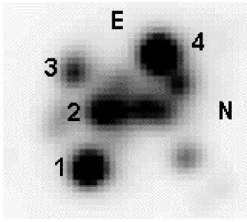
Figure 1: The HDE 269995 cluster in the LMC, from a section of an image taken in CTIO. S 111 is star number 1. The others were used for determining the foreground interstellar polarization towards S 111.

Table 1: Observed Optical Polarization Data for the Cluster

N	$P$ (%)	$\sigma_{P}$ (%)	$\theta$ ($\degr$)
1 (=S 111)	0.710	0.033	50.5
2	0.672	0.085	26.1
3	0.532	0.075	35.8
4	0.544	0.029	29.7

Table 2: Optical Polarization Data for S 111

OBSERVED				FOREGROUND				INTRINSIC
$P$ (%)	$\sigma_{P}$ (%)	$\theta$ ($\degr$)		$P$ (%)	$\sigma_{P}$ (%)	$\theta$ ($\degr$)		$P$ (%)	$\sigma_{P}$ (%)	$\theta$ ($\degr$)
0.710	0.033	50.5		0.552	0.026	30.0		0.467	0.042	75.3

3 Polarization and the B[e]SG envelopes

The envelopes of B[e]SG provide an ample opportunity for scattering of radiation from the central star due to the available free electrons, as revealed from their emission lines and near IR ($J$ band) excess, and dust, evidenced by their IR excess. Following M92, we reinvestigate the correlations between the optical polarization of B[e]SG and inferred electron densities and infrared excesses. This reanalysis is warranted by the additional data point S 111 provides, the recent finding concerning the binarity of AV 16/R 4 and newer photometric calibration tables for optical-near IR photometry.

3.1 Polarization and Electron density

It is believed that the $J$ excess from B[e]SG is due to free-free and bound-free radiation. Therefore, such excess is a measure of the electron density in the envelopes of B[e]SG (Zickgraf et al. z86 (1986), hereafter Z86). M92 correlated the polarization of nine MC B[e]SG with the electron density ($N_{e}$) obtained from $J$ excesses ($\Delta J$) by Z86. A measure of the optical magnitude needed to fit the stellar continuum energy distribution, and hence for obtaining $\Delta J$, is not available for S 111. Thus we estimated $N_{e}$ for S 111 not from $\Delta J$ but from the emission measure (EM) of H$\alpha$.

For estimating $N_{e}$ from H$\alpha$ we followed the method outlined by Z86. As a check on our procedure, we initially applied it to the other B[e]SGs, for which optical magnitudes are available. The first step required is obtaining the H$\alpha$ continuum flux. This was done using an interpolation of the fluxes in the $V$ and $I$ filters using the observed magnitudes of Z85, Z86 and Zickgraf et al. z89 (1989) (hereafter Z89) and a power law, $F_{\lambda}=k\lambda^{-\rm{n}}$. The exponent n was found to vary between 1.5 and 2.9 (with median = 2.5) for the different stars. The magnitudes were corrected for interstellar extinction, using the extinction curve of Code et al. (1976). The Galactic color excess $E(B-V)$ was taken as 0.05 (Z85, Bessell 1991 and Rodrigues et al. r97 (1997)) and the Magellanic color excess $E(B-V)$ from Z86 and Z89. The fluxes were then computed using the absolute fluxes of Bessell (1979). Our results compared well to those of Z89 within 30%.

For S 111, in order to calculate the H$\alpha$ continuum flux we estimated the magnitude of the object in the $V$ filter, using the bolometric correction $BC_{V}$ and the stellar luminosity by McGregor et al. (m88 (1988), hereafter M88), as well as the distance modulus for the LMC (Walker 1998). The estimated intrinsic (i.e., extinction corrected) apparent magnitude for S 111 thus found was 9.20 mag. This estimated $V$ magnitude is not quite consistent with the near infrared magnitudes of M88 (their Table 5). We did perform another estimate of the magnitude of S 111 using the photometry of Mendoza (1970), who obtained the magnitude in the $V$ filter for the cluster to which S 111 belongs. Our CCD images provide the relative fluxes of the brightest stars in the cluster. It was then possible to estimate the magnitude of S 111 from the cluster $V$ magnitude of Mendoza (1970) and our relative flux data. For this purpose, we assumed that the flux of the cluster was due to the contribution of its four brightest stars. From this assumption we obtained a new intrinsic magnitude for S 111, 10.26 (with an error of $\sim$0.02, the error in V for the S 111 cluster as estimated by Mendoza), a value more consistent with the near infrared magnitudes of S 111. Since there is no available $I$ filter measurement for S 111 either, the H$\alpha$ continuum flux of S 111 was obtained from an extrapolation of this $V$ flux assuming a value of n=2.5 for the index of the continuum flux distribution. A more definite estimate should probably be best done from direct filter photometry for S 111, specially in the $I$ filter.

The next step was obtaining the H$\alpha$ flux (H$\alpha$ continuum flux $\times$ equivalent width) and then the H$\alpha$ luminosity. For S 111, the equivalent width was measured from the H$\alpha$ profile given by Stahl & Wolf (1986) as 356 Å. The EM was calculated using the case B recombination theory formula (Osterbrock 1989). From the definition of EM, $N_{e}$ can be calculated as $\sqrt{\rm{EM}/\rm{V}}$, where V is the volume of the envelope. The shape of the envelope was taken as suggested by Z85. It consists of a disk with inner radius of 1 $R_{\star}$, outer radius of 300 $R_{\star}$ and thickness of 1 $R_{\star}$. For the stellar radius of S 111, we obtained the value of 148 $R_{\sun}$ using the effective temperature and stellar luminosity from M88. The resultant $N_{e}$ for S 111 was 0.43 $\times$ $10^{9}$ cm^-3.

As a check on the procedure, we reevaluated $N_{e}$ for other B[e]SG. The H$\alpha$ equivalent width of other B[e]SG stars were either taken from the literature (R 126, S 134 and S 12; Z89) or estimated by us (S 18, S 22 and R 66). Among the latter, two compared very well with the literature (S 18, Z89; S 22, Schulte-Ladbeck and Clayton 1993). Both the fluxes and EM values obtained by us agreed with those of Z86 and Z89 estimated from H$\alpha$. On the other hand, our values of $N_{e}$ differ some, though always of the same order of magnitude, from those of Z89’s obtained from $J$ excess. In general, the electron density from $\Delta J$ is on average two times larger than that of H$\alpha$. We hence used 0.8 $\times$ $10^{9}$ cm^-3 for the electron density in the envelope of S 111.

As discussed in detail by M92, high levels of intrinsic polarization are related to edge-on stars. We hence expect that polarization of these stars might be proportional to the electron density and the other stars (pole-on and intermediate-on) be distributed in a triangular pattern due to the dependence on $\sin^{2}$i, where i is the inclination angle through which the discs are seen. In Fig. 2 we plot the intrinsic polarization as a function of electron density. We use our $N_{e}$ value above for S 111 and Z89’s for the remaining stars. The polarization values are taken from Sect. 2 of this paper for S 111 and from M92 for the remaining objects.

Unlike M92, we have omitted from the plot in Fig. 2 the SMC star AV 16/R 4. Zickgraf et al. (1996a) have shown that this object is in fact a binary star, consisting of a B[e] star and an early A-type companion. The observed polarization of an object is basically the ratio between the scattered, polarized light from the circunstellar material and the total light from the system. Hence, such source of additional, unpolarized light in the system (i.e., the A component) would act to dilute an otherwise larger intrinsic polarization. In fact, of the four equator-on cases (as evidenced by their spectroscopic properties from the work of Zickgraf and collaborators) analysed by M92, R 4 showed the smallest intrinsic polarization. Interestingly, in addition to that, in the $P$ vs. $N_{e}$ correlation R 4 of M92 (his Fig. 4) R 4 clearly stood out from the other three equator-on cases by being well off the line defined by those objects.

We did a linear $\chi^{2}$ fit for the remaining spectroscopically edge-on stars (R 50, R 82 and S 22, filled squares in Fig. 2) and present that fit in Fig. 2. It can be seen that the remaining stars, i.e., the pole-on and intermediate stars, are distributed below this fit line, as expected. As in M92, we chose to use the Spearman rank-order correlation coefficient ($r_{s}$), to which a statistical significance can be attached. The calculated value of the $r_{s}$ for the P versus N_e correlation for all objects is 0.55, with a 12% probability, where a small probability means high significance. This indicates a moderate correlation between $P$ and $N_{e}$. Nevertheless this correlation is much higher than that of M92 (0.32 with 41%), which included R 4.

Figure 2: Intrinsic polarization versus electron density. The dotted line corresponds to a $\chi^{2}$ linear fit for edge-on stars (R 50, R 82 and S 22), indicated by the filled squares.

3.2 Color excess $\Delta(K-L)$

We can use the near-infrared color excess at wavelenghts longer than $J$ as a measure of dust emission (Z86, Z89). We define the following color excess $\Delta(K-L)$:

$$\Delta(K-L)=(K-L)_{\rm{corr}}-(K-L)_{\rm{int}}\,,$$ (2)

where $(K-L)_{\rm{corr}}$ is the observed color index $(K-L)$ corrected for interstellar extinction and $(K-L)_{\rm{int}}$ is the intrinsic color index due to the stellar contribution.

$(K-L)_{\rm{int}}$ was taken from the newly available $UBVRIJHKL$ color tables of Bessell et al. (1998). These tables take into account the star’s gravity, finer intervals of effective temperature and colors for T $>$ 21000K compared to those of Johnson (1966). $(K-L)_{\rm{corr}}$ was obtained using the observed magnitudes of Z85, Z86 and Z89, corrected by the interstellar color excesses taken from Z85 for the Galaxy and from Z86 and Z89 for the MC and using the extinction coefficients of Leitherer & Wolf (1984). We note that there might be probably uncertainties in the color excesses derived in these papers. The reason is that the dust envelope may also contribute to the observed reddening of the stellar spectrum. The amount of such reddening will depend on detailed modeling. The derived interstellar color excesses may then be considered as upper limits. One such example may be S 18, which has a derived $E(B-V)=0.40$ (Z89). Such a relatively large color excess, albeit possible, is rarely observed towards the SMC. Nevertheless, as expected, these color excesses have only a small effect in $(K-L)_{\rm{corr}}$ at these long, IR wavelengths.

In Fig. 3 we plot the intrinsic polarization as a function of the color excess $\Delta(K-L)$. As before, we omit R 4 from the correlation. A linear $\chi^{2}$ fit to the spectroscopically edge-on stars (R 50, R 82 and S 22) is also shown in the figure. It can be seen that not all stars are distributed below the fit line. The Spearman correlation coefficient for the P versus $\Delta(K-L)$ relation for all objects is 0.20, with a 60% probability. This value of $r_{s}$ shows a very weak correlation between $P$ and $\Delta(K-L)$.

Figure 3: Intrinsic polarization versus color excess. The dotted line as in Fig. 2.

In summary, the existing B[e]SG polarimetric data show that intrinsic polarization correlates better with electron density than dust scattering. This result is consistent with the spectropolarimetric observations of S 22 by Schulte-Ladbeck & Clayton (1993). They found that the polarizing mechanism in that object can be explained by electron scattering. Additional multifilter and spectropolarimetric measurements of the B[e]SG are clearly of the greatest interest. As discussed in M92, these measurements will allow an improved separation between intrinsic and foreground polarization as well as the detection of changes in polarization across spectral features produced in the B[e]SG envelopes. Such changes will help reveal the physical structure of their envelopes.

4 Monte Carlo models

In order to quantitatively infer consequences of the observed polarization to the B[e]SG envelopes, we used a Monte Carlo code developed by our group (Carciofi & Magalhães 2001). In this preliminary study, two geometries were chosen for these envelopes (although others may be used): cylindrical geometry and spherical geometry with density contrast. The density laws used were one of constant density and one proportional to $r^{-2}$. The codes perform the radiative transfer of the Stokes parameters ($I,Q,U,V$) for photons in scattering envelopes.

From the preceeding section, we found that polarization correlates best with electron density. We have hence only considered models with electron scattering at this point. We used data on nine B[e]SG for the models; that is, those from M92, with the exception of the binary AV 16/R 4, plus S 111. In Table 3 we summarize their stellar radius (Zickgraf 1990) and electron density values (Z89). For the modelling we considered five values for the average electron density in the envelope which encompass the observed ones (Table 3): [0.5, 1.5, 3, 4, 6] $\times$ $10^{9}$ cm^-3. The mean electron density for each case is calculated from $<N_{e}^{2}>$ (= EM/V), as described in Sect. 3.1. For the models, we have used the same approach, i.e., we calculated $<N_{e}^{2}>$ for a given geometry and density law and then took the square root of this value to represent the mean electron density of that specific model. In the figures of the models we use ${<N_{e}^{2}>}^{1/2}$ along the x-axis.

Table 3: Electron Densities and Stellar Radii for MC B[e]SG

Star	$R^{\rm a}$ $(R_{\sun})$	$N_{e}$b ($\times$ $10^{9}$ cm-3)
S 111	148c	0.8c
R 126	72	2.0
S 134	45	3.9
S 12	30	3.3
R 66	125	1.2
R 82∗	50	2.8
S 22∗	49	6.0
S 18	35	3.4
R 50∗	81	1.5

• stellar radii (Zickgraf 1990)

• electron density values (Z89)

• values obtained in this work

• edge-on stars

4.1 Cylindrical geometry

The envelope with cylindrical geometry was modeled adopting a stellar radius of 70 $R_{\sun}$, typical of a B[e]SG. The dimensions of the cylindrical disk are the same used earlier (Sect. 3.1), namely, inner radius $R_{i}$ = 1 $R_{\star}$, outer radius $R_{o}$ = 300 $R_{\star}$ and thickness of 1 $R_{\star}$.

The electron density law used was:

$$n_{e}(r)=\frac{\rm{K}}{r^{n}}\,,$$ (3)

where K is a constant and n is an exponent for constant ($n$=0) or variable ($n$=2) densities across the envelope. The constant K can be derived using the relation between the optical depth and the density law,

$$\tau=\int\limits^{R_{o}}_{R_{i}}\sigma_{\rm{T}}n_{e}(r)dr\,,$$ (4)

with $\sigma_{\rm{T}}$ being the Thomson scattering cross section.

4.1.1 Homogeneous density

In Fig. 4 we show the intrinsic polarization as a function of mean electron density (and equatorial optical depth) for a cylindrical disk with homogeneous density for several inclination angles. From the figure, we can note that these models fail to fit the observational data as most data points, including the edge-on objects, lie well above the curve i=90$\degr$, which is the maximum polarization predicted by the model. We conclude that homogeneous cylindrical envelopes are not a good representation for the MC B[e]SG envelopes.

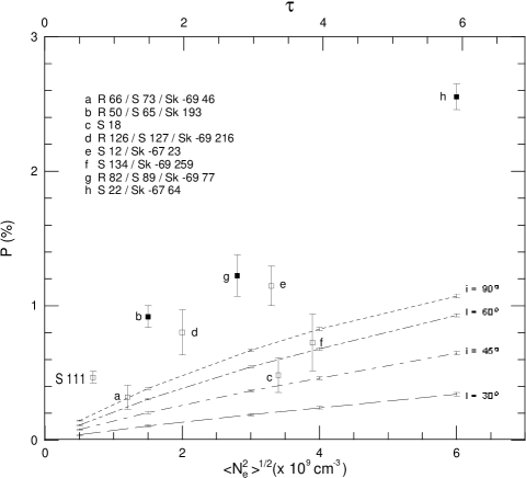
Figure 4: Intrinsic polarization of MC B[e]SG as a function of envelope mean electron density $N_{e}$ (= ${<N_{e}^{2}>}^{1/2}$) and equatorial optical depth $\tau$. Lines represent models with cylindrical geometry and homogeneous electron density for several inclination angles. The points with error bars correspond to polarimetric data from this paper (S 111) and M92 (other objects).

4.1.2 Density proportional to $r^{-2}$

The model results when the density falls with $r^{-2}$ are presented in Fig. 5. In the figure, most of the observational data points lie between the inclination angle curves i=20°and i=45°. In particular, the edge-on objects fall far from the i=90°curve. We conclude that, like the constant density models, the cylindrical $r^{-2}$ models do not fit well the observations either.

In order to investigate the dependence of the model results on the assumed stellar radius, we ran two additional cases, $R_{\star}$=30 $R_{\sun}$ and $R_{\star}$=140 $R_{\sun}$, which reasonably cover the range of MC B[e]SG radii (Table 3), for both constant and r^-2 density models. For the cases of constant density with $R_{\star}$=30 $R_{\sun}$, the model curves fall below all observed data points. The $R_{\star}$=140 $R_{\sun}$ model curves cover the $P-N_{e}$ data space better but still fail to adequately fit the edge-on cases. In addition, we know the edge-on objects do have in fact $R_{\star}$ between about 50 and 80 $R_{\sun}$ (Table 3). For the r^-2 density models, neither of these radius values fit the data points adequately.

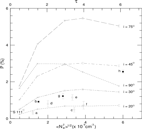
Figure 5: Intrinsic polarization of MC B[e]SG as a function of mean electron density square root $\sqrt{<N_{e}^{2}>}$ and equatorial optical depth $\tau$. Data are as in Fig. 4. Lines represent models with cylindrical geometry and electron density varying with $r^{-2}$ for several inclination angles.

In summary, we conclude that the models using cylindrical geometry do not fit with the data for B[e]SG, at least not for the dimensions that have been proposed (Z85).

4.2 Spherical geometry with density contrast

To model the spherical geometry with density contrast, we chose to use the parameterization of Waters et al. (1987), which has been also used by Wood et al. (1996). The equatorial-to-polar density ratio may in fact render this model more realistic for the B[e]SG.

The Waters et al. (1987) density law is

$$n_{e}(r)=n_{0}\left(\frac{R_{\star}}{r}\right)^{n}(1+A\sin^{m}\theta)\,,$$ (5)

where $n_{0}$ is the density in the stellar surface, $\theta$ is the polar angle. This parameterization consists of a spherically symmetric region combined with an equatorial disk in which $(1+A)$ determines the density contrast, between the pole and equator, and $m$ is a measure of the opening angle of the disk. The aperture angle at which the density is half its maximum value (measured from the equator) is:

$$\theta_{0}=\cos^{-1}(\frac{1}{2})^{1/m}.\$$ (6)

We have chosen to model two cases, that of an envelope with a constant density ($n$=0), and that with density proportional to $r^{-2}$ ($n$=2). In these cases, we used the same amount of mass as that of the scattering cylindrical disk. In doing that, the spherical envelope outer radius derived was 2850 $R_{\sun}$ ($\sim$41 $R_{\star}$) . Again, the stellar radius used in the models was 70 $R_{\sun}$.

4.2.1 Constant density

In the case of homogeneous density, we see that in eq. 5, $n_{e}(r)$ only depends on $\theta$, $m$ and $A$. We set the opening angle at $\theta$=5$\degr$, for which $m$=182. Zickgraf (1989) estimated disk opening angles of 20$\degr$ to 40$\degr$. We have run models with this range of values but the resulting polarization leves were too high (e.g., 7% for $N_{e}$ = 6 $\times$ $10^{9}$ cm^-3). The value of density contrast used was $10^{3}$ (Z86), which implies in $A$=999 in eq. 5.

In Fig. 6, we present the results for envelopes with the geometry parameterized with eq. 5 and constant electron density. These models provide a good fit to the observations, including the edge-on objects. We note that polarization level for i=90$\degr$ is larger than that obtained with cylindrical geometry (Fig. 4). This is due to the star, in the cylindrical geometry case, not being completely occulted by the envelope. The star then contributes with direct, non-polarized flux, lowering the resulting polarization level.

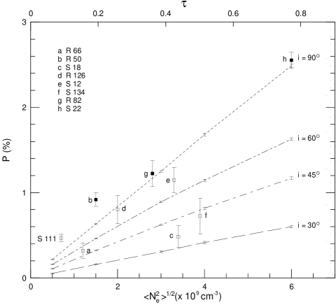
Figure 6: Intrinsic polarization of MC B[e]SG as a function of electron density $N_{e}$ (= ${<N_{e}^{2}>}^{1/2}$) and equatorial optical depth $\tau$. Data point are as in Fig. 4. Lines represent models with spherical geometry with density contrast and uniform electron density.

4.2.2 Density proportional to $r^{-2}$

With the density now proportional to $r^{-2}$, we use the same parameter set as for constant density. The model results are presented in Fig. 7. In the figure we can see that the model polarization obtained fall well below the expected level.

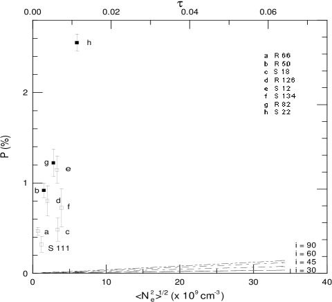
Figure 7: Intrinsic polarization of MC B[e]SG as a function of mean electron density square root $\sqrt{<N_{e}^{2}>}$ and the equatorial optical depth $\tau$. Data are the same of Fig. 4. Here we considered a spherical geometry with density contrast, and a $r^{-2}$ electron density.

5 Conclusions

We present optical polarization data for the LMC B[e]SG S 111. The estimated intrinsic polarization is (0.467 $\pm$ 0.042)% at 75$\aas@@fstack{\circ}$3. This polarization is consistent with the presence of a non-spherical circumstellar envelope around the object.

After excluding AV 16/R 4, a B[e]SG now known to be a binary, and with the inclusion of S 111, we found using more recent IR calibration data that intrinsic polarization correlates better with the electron density rather than the color excess $\Delta(K-L)$ in the envelopes of B[e]SG. This suggests that electron scattering is the main mechanism that causes polarization in the envelopes of these stars.

The spectroscopic data have been suggestive (Z85) of a two-component wind model for B[e]SG, i.e., a slow equatorial wind and a fast polar wind. We have hence considered two idealized models for such wind, one with a cylindrical geometry and another where the material is spherically distributed around the star but with a contrast enhancement along the equator. The results of our Monte Carlo modeling show that the spherical geometry with such density contrast fits the polarization observations very reasonably, being consistent with the two-component model for B[e]SG. In addition, the constant density case fits the data better than an $r^{-2}$ electron density law. This result agrees with the presence of a slow equatorial wind observed and modeled by Zickgraf et al. (1996b).

Questions still to be answered include details of the geometry of the equatorial disk, such as its opening angle, and the precise location of the scattering material within the disk. These will have to await spectropolarimetric observations of these objects. Changes (or the absence of them) in polarization accross spectral features, e.g., emission lines, would help us point out more precisely where the polarization arises in the envelope (decreases across emission line, for instance, would indicate that the polarization is produced closer to the star, etc.). Other spectropolarimetric features, such as changes across the Balmer discontinuities, might be helpful in assessing the envelope’s opening angle (e.g., Wood et al. 1997, for Be stars).

- (1) Appenzeller, I., Klare, G., Stahl, O., Wolf, B. & Zickgraf, F.-J. 1984, ESO Messenger 38, 28
- (2) Bessell, M.S. 1979, PASP 91, 589
- (3) Bessell, M.S. 1991, A&A 242, L17
- (4) Bessell, M.S., Castelli, F. & Plez, B. 1998, A&A 333, 231
- (5) Carciofi, A.C. & Magalhães, A.M. 2001, in preparation
- (6) Gummersbach, C., Zickgraf, F.-J. & Wolf, B. 1995, A&A 302, 409
- (7) Henize, K.G. 1956, ApJS 2, 315
- (8) Humphreys, R. & Davidson, K. 1979, ApJ 232, 409
- (9) Johnson, H. 1966, ARA&A 4, 193
- (10) Lamers, H., Zickgraf, F.-J., de Winter, D., Houziaux, L. & Zorec, J. 1998, A&A 340, 117
- (11) Leitherer, C. & Wolf, B. 1984, A&A 132, 151
- (12) Magalhães, A.M. 1992, ApJ 398, 286 (M92)
- (13) Magalhães, A.M., Benedetti, E. & Roland, E. 1984, PASP 96, 383
- (14) Magalhães, A.M., Rodrigues, C.V., Margoniner, V.E., Pereyra, A. & Heathcote, S. 1996, Polarimetry of the Interstellar Medium, ed. D.C.B. Whittet & W. Roberge (San Francisco: ASP), p. 118
- (15) McGregor, P., Hillier, D. & Hyland, A. 1988, ApJ 334, 639 (M88)
- (16) Mendoza, E. 1970, Bol. Obs. Tonantz. Tacub. 5, 269
- (17) Osterbrock, D. 1989, Astrophysics of Gaseous Nebulae, Freeman, San Francisco
- (18) Rodrigues, C.V., Magalhães, A.M., Coyne, G.V. & Piirola, V. 1997, ApJ 485, 618
- (19) Sanduleak, N. 1968, Contr. CTIO, No. 89
- (20) Schulte-Ladbeck, R. & Clayton, G. 1993, AJ 106, 790
- (21) Serkowski, K. 1974, in Methods of Experimental Physics, vol. 12, part A, eds. M.L. Meeks & N.P. Carleton (New York: Academic Press), p. 361
- (22) Stahl, O. & Wolf, B. 1986, A&A 158, 371
- (23) Walker, A. 1999, in: Post Hipparcos Cosmic Candles, eds. F. Caputo & A. Heck (Dordretch: Kluwer), ASSL 237, p. 125
- (24) Waters, L., Coté, J. & Lamers, H. 1987, A&A 185, 206
- (25) Wood, K., Bjorkman, K. & Bjorkman, J. 1997, ApJ 477, 926
- (26) Zickgraf, F.-J. 1989, in: Physics of Luminous Blue Variable, eds. K. Davidson, A. Moffat & H. Lamers (Dordretch: Kluwer), p. 117
- (27) Zickgraf, F.-J. 1990, in: Angular Momentum and Mass Loss for Hot Stars, eds. L.A. Willson & R. Stalio (Dordretch: Kluwer), NATO ASI Series 316, p. 245
- (28) Zickgraf, F.-J. 1999, in: Variable and Non-spherical Stellar Winds in Luminous Hot Stars, eds. B. Wolf, O. Stahl & A.W. Fullerton (Heidelberg: Springer), Lecture Notes in Physics Series, p. 40
- (29) Zickgraf, F.-J., Humphreys, R., Lamers, H., Smolinski, J., Wolf, B. & Stahl, O. 1996b, A&A 315, 510
- (30) Zickgraf, F.-J., Kovács, J., Wolf, B., Stahl, O., Kaufer, A. & Appenzeller, I. 1996a, A&A 309, 505
- (31) Zickgraf, F.-J., Wolf, B., Stahl, O. & Humphreys, R. 1989, A&A 220, 206 (Z89)
- (32) Zickgraf, F.-J., Wolf, B., Stahl, O., Leitherer, C. & Appenzeller, I. 1986, A&A 163, 119 (Z86)
- (33) Zickgraf, F.-J., Wolf, B., Stahl, O., Leitherer, C. & Klare, G. 1985, A&A 143, 421 (Z85)