Dark energy and the angular size - redshift diagram for milliarcsecond radio-sources

Abstract

We investigate observational constraints on the cosmic equation of state from measurements of angular size for a large sample of milliarcsecond compact radio-sources. The results are based on a flat Friedmann-Robertson-Walker (FRW) type models driven by non-relativistic matter plus a smooth dark energy component parametrized by its equation of state $p_{x}=\omega\rho_{x}$ ($-1\leq\omega<0$). The allowed intervals for $\omega$ and $\Omega_{\rm{m}}$ are heavily dependent on the value of the mean projected linear size $l$. For $l\simeq 20h^{-1}-30h^{-1}$ pc, we find $\Omega_{\rm{m}}\leq 0.62$, $\omega\leq-0.2$ and $\Omega_{\rm{m}}\leq 0.17$, $\omega\leq-0.65$ (68$\%$ c.l.), respectively. As a general result, this analysis shows that if one minimizes $\chi^{2}$ for the parameters $l$, $\Omega_{\rm{m}}$ and $\omega$, the conventional flat $\Lambda$CDM model ($\omega=-1$) with $\Omega_{\rm{m}}=0.2$ and $l=22.6h^{-1}$pc is the best fit for these angular size data.

A large number of recent observational evidences strongly suggest that we live in a flat, accelerating Universe composed by $\sim$ 1/3 of matter (barionic + dark) and $\sim$ 2/3 of an exotic component with large negative pressure, usually named dark energy or “quintessence”. The basic set of experiments includes: observations from SNe Ia (Perlmutter et al. 1998; 1999; Riess et al. 1998), CMB anisotropies (de Bernardis et al. 2000), large scale structure (Bahcall 2000), age estimates of globular clusters (Carretta et al. 2000; Krauss 2000; Rengel et al. 20001) and old high redshift galaxies (OHRG’s) (Dunlop 1996; Krauss 1997; Alcaniz & Lima 1999; Alcaniz & Lima 2001). It is now believed that such results provide the remaining piece of information connecting the inflationary flatness prediction ($\Omega_{\rm{T}}=1$) with astronomical observations, and, perhaps more important from a theoretical viewpoint, they have stimulated the current interest for more general models containing an extra component describing this unknown dark energy, and simultaneously accounting for the present accelerated stage of the Universe.

The absence of a convincing evidence concerning the nature of this dark component gave origin to an intense debate and mainly to many theoretical speculations in the last few years. Some possible candidates for “quintessence” are: a vacuum decaying energy density, or a time varying $\Lambda$-term (Ozer & Taha 1987; Freese 1987; Carvalho et al 1992, Lima and Maia 1994), a relic scalar field (Peebles & Ratra 1988; Frieman et al 1995; Caldwell et al 1998; Saini et al 2000) or still an extra component, the so-called “X-matter”, which is simply characterized by an equation of state $p_{x}=\omega\rho_{x}$, where $\omega\geq-1$ (Turner & White 1997; Chiba et al 1997) and includes, as a particular case, models with a cosmological constant ($\Lambda$CDM) (Peebles 1984). For “X-matter” models, several results suggest $\Omega_{x}\simeq 0.7$ and $\omega\leq-0.6$. For example, studies from gravitational lensing + SNe Ia provide $\omega\leq-0.7$ at 68$\%$ c.l. (Waga & Miceli 1999; see also Dev et al. 2001). Limits from age estimates of old galaxies at high redshifts require $\omega<-0.27$ for $\Omega_{\rm{m}}\simeq 0.3$ (Lima & Alcaniz 2000a). In addition, constraints from large scale structure (LSS) and cosmic microwave background anisotropies (CMB) complemented by the SN Ia data, require $0.6\leq\Omega_{x}\leq 0.7$ and $\omega<-0.6$ ($95\%$ c.l.) for a flat universe (Garnavich et al 1998; Perlmutter et al 1999; Efstathiou 1999), while for universes with arbitrary spatial curvature these data provide $\omega<-0.4$ (Efstathiou 1999).

On the other hand, although carefully investigated in many of their theoretical and observational aspects, an overview on the literature shows that a quantitative analysis on the influence of a “quintessence” component ($\omega={p_{x}}/{\rho_{x}}$) in some kinematic tests like angular size-redshift relation still remains to be analysed. Recently, Lima & Alcaniz (2000b) studied some qualitative aspects of this test in the context of such models, with particular emphasis for the critical redshift $z_{m}$ at which the angular size takes its minimal value. As a general conclusion, it was shown that this critical redshift cannot discriminate between world models since different scenarios can provide similar values of $z_{m}$ (see also Krauss & Schramm 1993). This situation is not improved even if evolutionary effects are taken into account. In particular, for the observationally favoured open universe ($\Omega_{\rm{m}}=0.3$) we found $z_{m}=1.89$, a value that can also be obtained for quintessence models having $0.85\leq\Omega_{x}\leq 0.93$ and $-1\leq\omega_{x}\leq-0.5$. Qualitatively, it was also argued that if the predicted $z_{m}$ is combinated with other tests, some interesting cosmological constraints can be obtained.

In this letter, we focus our attention on a more quantitative analysis. We consider the $\theta-z$ data of compact radio sources recently updated and extended by Gurvits et al. (1999) to constrain the cosmic equation of state. We show that a good agreement between theory and observation is possible if $\Omega_{\rm{m}}\leq 0.62$, $\omega\leq-0.2$ and $\Omega_{\rm{m}}\leq 0.17$, $\omega\leq-0.65$ (68$\%$ c.l.) for values of the mean projected linear size between $l\simeq 20h^{-1}-30h^{-1}$ pc, respectively. In particular we find that a conventional cosmological constant model ($\omega=-1$) with $\Omega_{\rm{m}}=0.2$ and $l=22.64h^{-1}$ pc is the best fit model for these data with $\chi^{2}=4.51$ for 9 degrees of freedom.

For spatially flat, homogeneous, and isotropic cosmologies driven by nonrelativistic matter plus an exotic component with equation of state, $p_{x}=\omega\rho_{x}$, the Einstein field equations take the following form:

$$({\dot{R}\over R})^{2}=H_{o}^{2}\left[\Omega_{\rm{m}}({R_{o}\over R})^{3}+\Omega_{x}({R_{o}\over R})^{3(1+\omega)}\right],$$ (1)

$${\ddot{R}\over R}=-{1\over 2}H_{o}^{2}\left[\Omega_{\rm{m}}({R_{o}\over R})^{3}+(3\omega+1)\Omega_{x}({R_{o}\over R})^{3(1+\omega)}\right],$$ (2)

where an overdot denotes derivative with respect to time, $H_{o}=100h{\rm{Kms^{-1}Mpc^{-1}}}$ is the present value of the Hubble parameter, and $\Omega_{\rm{m}}$ and $\Omega_{x}$ are the present day matter and quintessence density parameters. As one may check from (1) and (2), the case $\omega=-1$ corresponds effectively to a cosmological constant.

In such a background, the angular size-redshift relation for a rod of intrinsic length $l$ can be written as (Sandage 1988)

$$\theta(z)={D(1+z)\over\xi(z)}\quad.$$ (3)

In the above expression $D$ is the angular-size scale expressed in milliarcseconds (marcs)

$$D={100lh\over c},$$ (4)

where $l$ is measured in parsecs (for compact radio-sources), and the dimensionless coordinate $\xi$ is given by (Lima & Alcaniz 2000b)

$$\xi(z)=\int_{(1+z)^{-1}}^{1}{dx\over x\left[\Omega_{\rm{m}}x^{-1}+(1-\Omega_{\rm{m}})x^{-(1+3\omega)}\right]^{{1}\over{2}}}.$$ (5)

The above equations imply that for given values of $l$, $\Omega_{\rm{m}}$ and $\omega$, the predicted value of $\theta(z)$ is completely determined. Two points, however, should be stressed before discussing the resulting diagrams. First of all, the determination of $\Omega_{\rm{m}}$ and $\omega$ are strongly dependent on the adopted value of $l$. In this case, instead of assuming a especific value for the mean projected linear size, we have worked on the interval $l\simeq 20h^{-1}-30h^{-1}$ pc, i.e., $l\sim O(40)$ pc for $h=0.65$, or equivalently, $D=1.4-2.0$ marcs. Second, following Kellermann (1993), we assume that possible evolutionary effects can be removed out from this sample because compact radio jets are (i) typically less than a hundred parsecs in extent, and, therefore, their morphology and kinematics do not depend considerably on the intergalactic medium and (ii) they have typical ages of some tens of years, i.e., they are very young compared to the age of the Universe.

In our analysis we consider the angular size data for milliarcsecond radio-sources recently compiled by Gurvits et al. (1999). This data set, originally composed by 330 sources distributed over a wide range of redshifts ($0.011\leq z\leq 4.72$), was reduced to 145 sources with spectral index $-0.38\leq\alpha\leq 0.18$ and total luminosity $Lh^{2}\geq 10^{26}$ W/Hz in order to minimize any possible dependence of angular size on spectral index and/or linear size on luminosity. This new sample was distributed into 12 bins with 12-13 sources per bin (see Fig. 1). In order to determine the cosmological parameters $\Omega_{\rm{m}}$ and $\omega$, we use a $\chi^{2}$ minimization neglecting the unphysical region $\Omega_{\rm{m}}<0$,

$$\chi^{2}(l,\Omega_{\rm{m}},\omega)=\sum_{i=1}^{12}{\frac{\left[\theta(z_{i},l,\Omega_{\rm{m}},\omega)-\theta_{oi}\right]^{2}}{\sigma_{i}^{2}}},$$ (6)

where $\theta(z_{i},l,\Omega_{\rm{m}},\omega)$ is given by Eqs. (3) and (5) and $\theta_{oi}$ is the observed values of the angular size with errors $\sigma_{i}$ of the $i$th bin in the sample.

Figure 1 displays the binned data of the median angular size plotted against redshift. The curves represent flat quintessence models with $\Omega_{\rm{m}}=0.3$ and some selected values of $\omega$. As discussed in Lima & Alcaniz (2000b), the standard open model (thick line) may be interpreted as an intermediary case between $\Lambda$CDM ($\omega=-1$) and quintessence models with $\omega\leq-0.5$. In Fig. 2 we show contours of constant likelihood (95$\%$ and 68$\%$) in the plane $\omega-\Omega_{\rm{m}}$ for the interval $l\simeq 20h^{-1}-30h^{-1}$ pc. For $l=20.58h^{-1}$ pc ($D=1.4$ marcs), the best fit occurs for $\Omega_{\rm{m}}=0.26$ and $\omega=-0.86$. As can be seen there, this assumption provides $\Omega_{\rm{m}}\leq 0.48$ and $\omega=-0.3$ at 1$\sigma$. In the subsequent panels of the same figure similar analyses are displayed for $l\simeq 22.05h^{-1}$ pc ($D=1.5$ marcs), $l\simeq 23.53h^{-1}$ pc ($D=1.6$ marcs) and $l\simeq 29.41h^{-1}$ pc ($D=2.0$ marcs), respectively. As should be physically expected, the limits are now much more restrictive than in the previous case because for the same values of $\theta_{oi}$ it is needed larger $\xi(z)$ (for larger $l$) and, therefore, smaller values of $\omega$. For $l\simeq 29.41h^{-1}$ pc, we find $\Omega_{\rm{m}}=0.04$ and $\omega=-1$ as the best fit model. For intermediate values of $l$, namely, $l=22.0h^{-1}$ pc ($D=1.5$ marcs) and $l=23.5h^{-1}$ pc ($D=1.6$ marcs), we have $\Omega_{\rm{m}}=0.22$, $\omega=-0.98$ and $\Omega_{\rm{m}}=0.16$ and $\omega=-1$, respectively. In particular, for smaller values of $l$, e.g., $l\simeq 14.70h^{-1}$ pc ($D=1.0$ marcs) we find $\Omega_{\rm{m}}=0.36$, $\omega=-0.04$. As a general result (independent of the choice of $l$), if we minimize $\chi^{2}$ for $l$, $\Omega_{\rm{m}}$ and $\omega$, we obtain $l=22.64h^{-1}$ pc ($D=1.54$ marcs), $\Omega_{\rm{m}}=0.2$ and $\omega=-1$ with $\chi^{2}=4.51$ for 9 degrees of freedom (see Table 1). It is worth notice that our results are rather different from those presented by Jackson & Dodgson (1996) based on the original Kellermann’s data (Kellermann 1993). They argued that the Kellermann’s compilation favours open and highly decelerating models with negative cosmological constant. Later on, they considered a bigger sample of 256 sources selected from the compilation of Gurvits (1994) and concluded that the standard flat CDM model is ruled out at $98.5\%$ confidence level whereas low-density models with a cosmological constant of either sign are favoured (Jackson & Dodgson 1997). More recently, Vishwakarma (2001) used the updated data of Gurvits et al. (1999) to compare varying and constant $\Lambda$CDM models. He concluded that flat $\Lambda$CDM models with $\Omega_{\rm{m}}=0.2$ are favoured.

At this point it is also interesting to compare our results with some recent determinations of $\omega$ derived from independent methods. Recently, Garnavich et al. (1998) using the SNe Ia data from the High-Z Supernova Search Team found $\omega<-0.55$ ($95\%$ c.l.) for flat models whatever the value of $\Omega_{\rm{m}}$ whereas for arbitrary geometry they obtained $\omega<-0.6$ ($95\%$ c.l.). As commented there, these values are inconsistent with an unknown component like topological defects (domain walls, string, and textures) for which $\omega=-\frac{n}{3}$, being $n$ the dimension of the defect. The results by Garnavich et al. (1998) agree with the constraints obtained from a wide variety of different phenomena (Wang et al. 1999), using the “concordance cosmic” method. Their combined maximum likelihood analysis suggests $\omega\leq-0.6$, which is less stringent than the upper limits derived here for values of $l\geq 20h^{-1}$ pc. More recently, Balbi et al. (2001) investigated CMB anisotropies in quintessence models by using the MAXIMA-1 and BOOMERANG-98 published bandpowers in combination with the COBE/DMR results (see also Corasaniti & Copeland 2001). Their analysis sugests $\Omega_{x}>0.7$ and $-1\leq\omega\leq-0.5$ whereas Jain et al (2001) found, by using image separation distribution function of lensed quasars, $-0.75\leq\omega\leq-0.42$, for the observed range of $\Omega_{m}\sim 0.2-0.4$ (Dekel et al. 1997). These and other recents results are summarized in Table 2.

Let us now discuss briefly these angular size constraints whether the adopted X-matter model is replaced by a scalar field motivated cosmology, as for instance, that one proposed by Peebles and Ratra (1988). These models are defined by power law potentials, $V(\phi)\sim\phi^{-\alpha}$, in such a way that the parameter of the effective equation of state ($w_{\phi}=p_{\phi}/\rho_{\phi}$) may become constant at late times (or for a given era). In this case, as shown elsewhere (Lima & Alcaniz 2000c), the dimensionless quantity $\xi$ defining the angular size reads

$$\xi(z)=\int_{(1+z)^{-1}}^{1}{dx\over x[\Omega_{\rm{m}}x^{-1}+(1-\Omega_{\rm{m}})x^{{{4-\alpha}\over{2+\alpha}}}]^{{1}\over{2}}}.$$ (7)

Comparing the above expression with (5) we see that if $\omega=-{2/(2+\alpha)}$ this class of models may reproduce faithfully the X-matter constraints based on the angular size observations presented here. However, as happens with the Supernovae type Ia data (Podariu & Ratra 2000), the two sets of confidence contours may differ significantly if one goes beyond the time independent equation of state approximation. Naturally, a similar behavior is expected if generic scalar field potentials are considered.

Finally, we stress that measurements of angular size from distant sources provide an important test for world models. However, in order to improve the results a statistical study describing the intrinsic lenght distribution of the sources seems to be of fundamental importance. On the other hand, in the absence of such analysis but living in the era of precision cosmology, one may argue that reasonable values for astrophysical quantities (like the characteristic linear size $l$) can be infered from the best cosmological model. As observed by Gurvits (1994), such an estimative could be useful for any kind of study envolving physical parameters of active galactic nuclei (AGN). In principle, by knowing $l$ and assuming a physical model for AGN, a new method to estimate the Hubble parameter could be established.

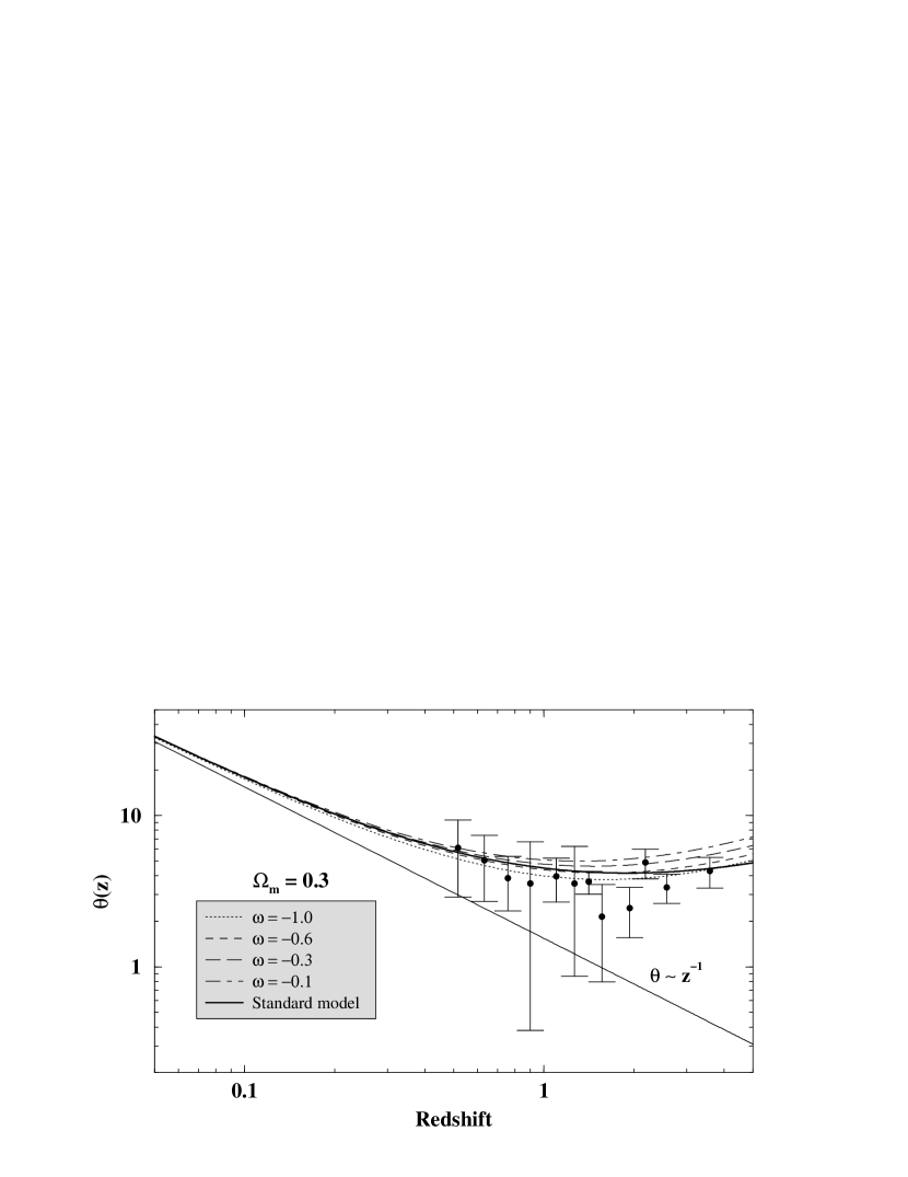
Figure 1: Angular size versus redshift for 145 sources binned into 12 bins (Gurvits et al. 1999). The curves correspond to the characteristic linear size $l=22.64h^{-1}$ pc. Thick solid curve is the prediction of the standard open model ($\Omega_{\rm{m}}=0.3$).

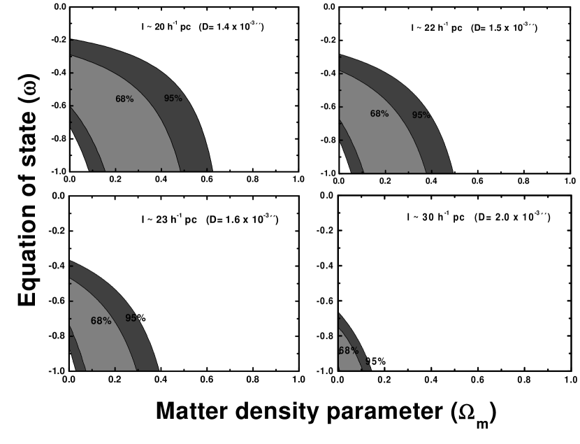
Figure 2: Confidence regions in the $\omega-\Omega_{m}$ plane according to the updated sample of angular size data (Gurvits et al. 1999). The solid lines in each panel show the 95$\%$ and 68$\%$ likelihood contours for flat quintessence models.

$D$ (mas)	$lh$ (pc)	$\Omega_{\rm{m}}$	$\omega$	$\chi^{2}$
1.4	20.58	0.26	-0.86	4.56
1.5	22.05	0.22	-0.98	4.52
1.6	23.53	0.16	-1	4.54
2.0	29.41	0.04	-1	5.57
Best fit: 1.54	22.64	0.2	-1	4.51

Table 1: Limits on $\omega$ from $\theta-z$ relation

Method	Author	$\Omega_{\rm{m}}$	$\omega$
CMB+SNe Ia..	Turner & White (1997)	$\simeq 0.3$	$\simeq-0.6$
	Efstathiou (1999)	$\sim$	$<-0.6$
SNe Ia…………	Garnavich et al. (1998)	$\sim$	$<-0.55$
SGL+SNe Ia..	Waga & Miceli (1999)	$0.24$	$<-0.7$
SNe Ia+LSS…	Perlmutter et al. (1999)	$\sim$	$<-0.6$
Various…………	Wang et al. (1999)	$0.2-0.5$	$<-0.6$
OHRG‘s……….	Lima & Alcaniz (2000a)	$0.3$	$\leq-0.27$
CMB……………	Balbi et al. (2001)	$0.3$	$\leq-0.5$
	Corasaniti & Copeland (2001)	$\sim$	$\leq-0.96$
SGL…………….	Jain et al. (2001)	$0.2-0.4$	$\geq-0.75$, $\leq-0.55$

Table 2: Limits to $\omega$ for a given $\Omega_{\rm{m}}$

References

- (1) Alcaniz J. S. & Lima J. A. S. 1999, ApJ, 521, L87
- (2) Alcaniz J. S. & Lima J. A. S. 2001, ApJ, 550, L133
- (3) Balbi A., Baccigalupi C., Matarrese S., Perrotta F., Vittorio N. 2001, ApJ 547 L89
- (4) Caldwell R. R., Dave R. & Steinhardt P. J. 1998, Phys. Rev. Lett. 80, 1582
- (5) Carretta E. et al. 2000, ApJ, 533, 215
- (6) Carvalho J. C., Lima J. A. S. & Waga I. 1992, Phys. Rev. D46, 2404
- (7) Chiba T., Sugiyama N. & Nakamura T. 1997, MNRAS, 289, L5
- (8) Corasaniti P. S. & Copeland E. J. 2001, preprint (astro-ph/0107378)
- (9) de Bernardis P. et al. 2000, Nature, 404, 955
- (10) Dekel A., Burstein D. & White S., In Critical Dialogues in Cosmology, edited by N. Turok World Scientific, Singapore (1997)
- (11) Dev A., Jain D., Panchapakesan N., Mahajan M. & Bhatia V. 2001, preprint (astro-ph/0104076)
- (12) Dunlop J. S. et al. 1996, Nature, 381, 581
- (13) Efstathiou G. 1999, MNRAS, 310, 842
- (14) Freese K., Adams F. C., Frieman J. A. & Mottola E. 1987, Nucl. Phys. B287, 797
- (15) Frieman J. A. , Hill C. T., Stebbins A. & Waga I. 1995, Phys. Rev. Lett. 75, 2077
- (16) Garnavich P. M. et al. 1998, ApJ, 509, 74
- (17) Gurvits L. I. 1994, Ap. J. 425, 442
- (18) Gurvits L. I., Kellermann K. I. & Frey S. 1999, A&A 342, 378
- (19) Jackson J. C. & Dodgson M. 1997, MNRAS 278, 603
- (20) Jackson J. C. & Dodgson M. 1997, MNRAS 285, 806
- (21) Jain D., Dev A., Panchapakesan N., Mahajan M. & Bhatia V. 2001, preprint (astro-ph/0105551)
- (22) Kellermann K. I. 1993, Nature 361, 134
- (23) Krauss L. M. & Schramm D. N. 1993, ApJ 405, L43
- (24) Krauss L. M. 1997, ApJ, 480, 466
- (25) Krauss L. M. 2000, Phys. Rep. 333, 33
- (26) Lima J. A. S. & Maia J. M. F. 1994, Phys. Rev D49, 5597
- (27) Lima J. A. S. & Alcaniz J. S. 2000a, MNRAS, 317, 893
- (28) Lima J. A. S. & Alcaniz J. S. 2000b, A&A, 357, 393
- (29) Lima J. A. S. & Alcaniz J. S. 2000c, Gen. Rel. Grav. 32, 1851
- (30) Ozer M. & Taha O. 1987, Nucl. Phys., B287, 776
- (31) Peebles P. J. E. 1984, ApJ 284, 439
- (32) Peebles P. J. E. & Ratra B. 1988, ApJ 325, L17
- (33) Podariu S. & Ratra B. 2000, ApJ 532, 109
- (34) Perlmutter S., et al. 1998, Nature, 391, 51
- (35) Perlmutter S., et al. 1999, ApJ, 517, 565
- (36) Perlmutter S., Turner M. S. & White M. 1999, Phys. Rev. Lett., 83, 670
- (37) Ratra B. & Peebles P. J. E. 1988, Phys. Rev. D37, 3406
- (38) Rengel M., Mateu J. & Bruzual G. 2001, IAU Symp. 207, Extragalactic Star Clusters, Eds. E. Grebel, D. Geisler, D. Minniti (in press), preprint (astro-ph/0106211)
- (39) Riess A. et al. 1998, AJ, 116, 1009
- (40) Saini T. D., Raychaudhury S., Sahni V. & Starobinsky A. A. 2000, Phys. Rev. Lett. 85, 1162
- (41) Turner M. S. & White M. 1997, Phys. Rev. D56, R4439
- (42) Sandage A. 1988, Ann. Rev. Astron. Astrophys. 26, 561
- (43) Vishwakarma R. G. 2001, Class. Quant. Grav. 18, 1159
- (44) Waga I. & Miceli A. P. M. R. 1999, Phys. Rev D59, 103507
- (45) Wang L., Caldwell R. R., Ostriker J. P., & Steinhardt P. J. 2000, ApJ 530, 17