The ionization fraction in $\alpha$–models of protoplanetary disks

Abstract

We calculate the ionization fraction of protostellar $\alpha$ disks, taking into account vertical temperature structure, and the possible presence of trace metal atoms. Both thermal and X–ray ionization are considered. Previous investigations of layered disks used radial power–law models with isothermal vertical structure. But $\alpha$ models are used to model accretion, and the present work is a step towards a self-consistent treatment. The extent of the magnetically uncoupled (“dead”) zone depends sensitively on $\alpha$, on the assumed accretion rate, and on the critical magnetic Reynolds number, below which MHD turbulence cannot be self–sustained. Its extent is extremely model-dependent. It is also shown that a tiny fraction of the cosmic abundance of metal atoms can dramatically affect the ionization balance. Gravitational instabilities are an unpromising source of transport, except in the early stages of disk formation.

1 Introduction

The only process known that is able to initiate and sustain turbulent transport in accretion disks is the magnetorotational instability (MRI; Balbus & Hawley 1991, 1998 and references therein). Because of the presence of finite resistivity, however, protostellar disk applications of the MRI are not straightforward. Numerical magnetohydrodynamic (MHD) disk simulations with Ohmic dissipation (Fleming et al. 2000) show that magnetic turbulence cannot be sustained if the magnetic Reynolds number, $Re_{M}$, is lower than some critical value, $Re_{M,{\rm crit}}$. If there is a net magnetic flux through the disk, the simulations indicate that $Re_{M,{\rm crit}}$ is about 100, and roughly corresponds to the Reynolds number below which the modes are linearly stable. If there is no net magnetic flux through the disk, $Re_{M,{\rm crit}}$ is found to be much larger, on the order of $10^{4}$. In this case, MHD turbulence can be suppressed even if the linear modes are only slightly affected. It is important to bear in mind that the value of $Re_{M,{\rm crit}}$ is uncertain. Recent studies of the linear stability of protostellar disks indicate that the effects of Hall electromotive forces are important, and that the actual critical Reynolds number may accordingly be smaller (Wardle 1999, Balbus & Terquem 2001).

On scales of 1 AU in a protostellar disk, $Re_{M}=100$ corresponds to ionization fraction of about $10^{-12}$ (e.g., Balbus & Hawley 2000 and § 4 below). Although very small, this fraction may not be attained in the intermediate regions of protostellar disks. The disk zones in which $Re_{M}$ is lower or larger than the critical Reynolds number are usually referred to as dead and active, respectively (Gammie 1996). The active layer extends vertically from the disk surface down to some altitude, which depends upon the radial location and the disk model.

The extent of the dead zone has been modeled by several authors using different ionization agents: Gammie (1996, cosmic rays), Igea & Glassgold (1999, X-rays) and Sano et al. (2000, cosmic rays and radioactivity). All these studies were based on the minimum mass disk model of Hayashi, Nakazawa & Nakagawa (1985), in which temperature and surface mass density vary as a simple power law of the radius, and the vertical structure is isothermal. This is a rather arbitrary choice, and the large scale structure of a turbulent $\alpha$ disk is in fact very different (Papaloizou & Terquem 1999). There is some theoretical evidence that MHD turbulence leads to a large scale $\alpha$ type structure in thin Keplerian disks (Balbus & Papaloizou 1999). It is the goal of this paper to investigate the ionization fraction of an $\alpha$–type disk, taking into account the vertical structure of such models. We shall consider thermal ionization and X–ray ionization, as these mechanisms are likely to be more important than cosmic rays in X-ray active young stellar objects (Glassgold, Feigelson & Montmerle 2000).

The disk ionization depends on the recombination rate of the electrons, which are removed through dissociative recombination with molecular ions and, at a much slower rate, through radiative recombination with heavy metal ions. In the previous studies of disk ionization by X–rays, it was assumed that all the metal atoms were locked up in dust grains most of which had themselves sedimented toward the disk midplane. However, the ionization fraction is extremely sensitive to even a very small number of metal atoms. This is because these rapidly pick up the charges of molecular ions and recombine only slowly with the electrons. In this paper, we therefore include the effect of a non zero density of metal atoms on the disk ionization.

The plan of the paper is as follows: In § 2, we describe the disk models used, and compare them with Hayashi et al. (1985). In § 3, we discuss the different ionization mechanisms. Thermal ionization is important in the disk inner parts, whereas X–ray ionization dominates everywhere else. We also discuss the effect of the presence of heavy metal atoms on the ionization fraction. In § 4 we present results for $\alpha$–type disks for a range of gas accretion rate $\dot{M}$ and values of the viscosity parameter $\alpha$. We find that the extent of the dead zone depends very sensitively on the critical Reynolds number, the parameters of the disk model ($\dot{M}$ and $\alpha$) and the density of heavy metal atoms. With no metal atoms and $Re_{M,{\rm crit}}=100$, we find in most cases that the dead zone generally extends from a fraction of an AU out to $10$ to $10^{2}$ AU. With an accretion rate of $\dot{M}=10^{-8}$ M_⊙ yr^-1 and $\alpha=10^{-2}$ for instance, the dead zone extends from 0.2 to 100 AU. This is much larger than what was found by previous authors, who used a smaller value of $Re_{M,{\rm crit}}$. However, we also find that the dead zone disappears completely for $\alpha\geq 10^{-2}$ when there is even a tiny density of heavy metal atoms. For instance, a density as small as $10^{-7}$ or $10^{-6}$ times the cosmic abundance is enough to make a disk with $\dot{M}=10^{-8}$ M_⊙ yr^-1 and $\alpha=10^{-2}$ completely turbulent. The dead zone is dramatically reduced or even disappears when the critical Reynolds number is taken to be 1, even when there are no heavy metal atoms. In § 5, we study the evolution of an $\alpha$ disk with a dead zone, with the aim of investigating local gravitational instability. Gammie (1996, 1999) and Armitage, Livio & Pringle (2001) have noted that a layered disk cannot accrete mass steadily, and that accumulation of mass in the dead zone may lead to gravitational instabilities. We find that when there is no mass falling onto the disk, the accumulation rate is too slow for gravitational instabilities to develop within the disk lifetime. Finally, in § 6 we summarize and discuss our results.

2 Disk models

We use conventional $\alpha$–disk models, as calculated by Papaloizou & Terquem (1999), to which the reader is referred for details. The disk is assumed to be in Keplerian rotation around a central mass $M_{\ast}=1$ M_⊙. The opacity, taken from Bell & Lin (1994), has contributions from dust grains, molecules, atoms and ions. The values of $\alpha$ and mass flow rate $\dot{M}$ are taken to be free parameters, and determine the model uniquely. In the steady state limit, $\dot{M}$ is constant through the disk. At a given radius $r$, the vertical structure is obtained by solving the equations of hydrostatic equilibrium, energy conservation and radiative transport with appropriate boundary conditions. (At the temperatures of interest here, convective transport is not significant). The detailed results of these calculations for $\alpha=10^{-2}$ or 0.1 and $\dot{M}$ in the range $10^{-9}$–$10^{-6}$ M_⊙ yr^-1 may be found in Papaloizou & Terquem (1999). In Figure 1, we plot steady state values of the midplane temperature $T_{m}$ and the surface mass density $\Sigma$ versus $r$ for $\alpha$ between $10^{-3}$ and $10^{-1}$; for illustrative purposes we have adopted $\dot{M}=10^{-8}$ M_⊙ yr^-1.

All solar nebula ionization studies previous to this have used the Hayashi et al. (1985) model of the solar nebula:

$$\Sigma=1700\left(\frac{1\;{\rm AU}}{r}\right)^{1.5}\;{\rm g~{}cm}^{-2}\;\;{\rm and}\;\;T=280\left(\frac{1\;{\rm AU}}{r}\right)^{0.5}\;{\rm K},$$

as the equilibrium profile. (Here, $r$ is the cylindrical radius.) This model is based upon chain of arguments: the current orbits and composition of the planets reflect the distribution and composition of dust in the preplanetary nebula; the planets have not moved radially in the course of their history; the formation of planets was extremely efficient. While this has been an useful organization of a complex problem, it certainly leaves room for other approaches to modeling the nebula. A question of some interest is how important the nebular model is to the ionization structure, which has motivated the approach presented here. For example, the Hayashi et al. (1985) model leads to a more centrally condensed disk mass than that obtained in a steady $\alpha$–disk. With $\alpha=10^{-2}$, a very large accretion rate of $\dot{M}\sim 10^{-6}$ M_⊙ yr^-1 is necessary to obtain the above Hayashi value of $\Sigma$ at 1 AU. For comparison, we have plotted temperature and mass density curves of the two models in Figure 1.

Ionization by X–rays is thus much more efficient around 1 AU in an $\alpha$–disk model than in the Hayashi et al. (1985) model. The theoretical justification for a minimum mass model is not strongly compelling, and it is quite incompatible with standard accretion disk theory. In addition, as mentioned above, there is some theoretical evidence that MHD turbulence leads to a large scale $\alpha$ type structure in thin Keplerian disks (Balbus & Papaloizou 1999). This is the primary motivation for the work presented here.

3 Ionization and Recombination

Protostellar disks are ionized mainly by thermal processes and by nonthermal X–rays. Cosmic rays, a classical ionization source in cool gas, have also been considered as a source of ionization (Gammie 1996, Sano et al. 2000), but the low energy particles (important for ionization) were almost certainly excluded by winds from the early solar nebula, as they are today in a far less active environment. Radioactive decay of ⁴⁰K and ²⁶Al has also been investigated by some authors (e.g., Consolmagno & Jokipii 1978), but their ionization effects are quite small compared to the levels of interest here (Stepinski 1992, Gammie 1996).

3.1 Thermal ionization

If not condensed onto grains, the alkali ions Na⁺ and K⁺ will be the dominant thermal ionization source in protostellar disks (Umebayashi & Nakano 1983). At the onset of dynamically interesting ionization levels ($\sim 10^{-13}$), the K⁺ ion is, with its smaller ionization potential, more important. In this regime, the Saha equation may be approximated as (Balbus & Hawley 2000):

$$x_{e}\equiv\frac{n_{e}}{n_{n}}=6.47\times 10^{-13}\left(\frac{a}{10^{-7}}\right)^{1/2}\left(\frac{T}{10^{3}}\right)^{3/4}\left(\frac{2.4\times 10^{15}}{n_{n}}\right)^{1/2}\frac{{\rm exp}\left(-25188/T\right)}{1.15\times 10^{-11}}$$ (1)

where $n_{e}$ and $n_{n}$ are respectively the electron and neutral number densities in cm^-3, and $a$ is the K abundance relative to hydrogen. Due to the Boltzmann cut–off factor, thermal ionization is important only in the disk inner regions, on scales less than an AU, where the midplane temperature is likely to exceed $10^{3}$ K. (Above this temperature the alkalis will tend to be in the gas phase, making the approximation self-consistent.) If there is magnetic coupling on scales larger than this, nonthermal ionization sources are required.

3.2 X–ray ionization

Young stellar objects appear to be very active X-ray sources, with X-ray luminosities in the range of $10^{29}$–$10^{32}$ erg s^-1 and photon energies from about 1 to 5 keV (Koyama et al. 1994, Casanova et al. 1995, Carkner et al. 1996). Glassgold, Najita & Igea (1997, hereafter GNI97, see also Igea & Glassgold 1999) pointed out that these X-rays are likely to be the dominant nonthermal ionization source in protostellar disks. These authors modeled the X-ray source as an isothermal ($T=T_{X}$) bremsstrahlung coronal ring, of radius of about $10~{}R_{\odot}$, located at a similar distance above (and below) the disk midplane. The total X-ray luminosity is $L_{X}$, with each hemisphere contributing $L_{X}/2$. The associated ionization rate is given by (Krolik & Kallman 1983, GNI97):

$$\zeta=\frac{(L_{X}/2)}{4\pi r^{2}kT_{X}}\;\sigma\left(kT_{X}\right)\;\frac{kT_{X}}{\Delta\epsilon}\;J(\tau).$$ (2)

Here, $\sigma$ is the photoionization cross section, which is fit to a power law (Igea & Glassgold 1999):

$$\sigma(E)=8.5\times 10^{-23}(E/{\rm keV})^{-n},$$ (3)

with $n=2.81$ (these values apply to the case where heavy elements are depleted onto grains and get segregated from the gas). $\Delta\epsilon=37$ eV is the average energy required by a primary photoelectron to make a secondary ionization. The dimensionless integral $J$ is

$$J(\tau)=\int^{\infty}_{x_{0}}x^{-n}\exp(-x-\tau x^{-n})\,dx,$$ (4)

an energy integral over the X-ray spectrum involving the product of the cross section (whence the factor $x^{-n}$) and the attenuated X-ray flux. The factor $\tau$ is the optical depth at an energy of $kT_{X}$; it depends upon one’s location within the disk. Generally the integral is insensitive to the lower limit threshold energy represented by $x_{0}$, and for the large $\tau$ case of interest here, it may be asymptotically expanded. The leading order result is

$$J(\tau)\simeq A\tau^{-a}\exp(-B\tau^{-b})$$ (5)

where $A=0.686$, $B=1.778$, $a=0.606$, $b=0.262$. In computing the optical depth, we make the approximation that the photons travel along straight lines; that is, we will neglect their diffusion both by the ambient medium and by the disk interior. Note however that scattering by the disk atmosphere would increase the ionization, both because some of the photons directed away from the disk would be scattered back, and because scattering provides pathways to the disk interior with smaller optical depths than a simple linear traversal. Note that here we do not make the approximation of GNI97 that the path of the photons inside the disk is vertical.

3.3 Recombination processes

In contrast to ionization, which is reasonably straightforward, electron recombination is greatly complicated by the presence of dust grains in the nebula. Not only are results dependent upon the size spectrum of the grains, imperfectly understood surface physicochemical processes will strongly influence charge capture and emission. Uncertainties attending the role of dust grains represent the greatest obstacle in estimating the solar nebula’s ionization structure.

Gammie (1996) and GNI97 finessed this issue by arguing that the dust will settle rapidly toward the midplane, and that the dominant recombination process will therefore be molecular dissociative recombination. While this greatly simplifies matters, it is prudent to regard the vertical distribution of the grains in magnetically coupled disk regions as an outstanding problem. Turbulence tends to mix, but the MRI is not particularly efficient at mixing vertically. Convective turbulence, should it be present, is a fine vertical mixer, and dust emission in the upper layers enhances the cooling, aiding the convection process itself. But sustaining convection without the MRI is known to be problematic.

Given the uncertainties, we take the view that it makes little sense to strive for high accuracy in a complex model. We have therefore opted for the simplicity of the previous studies, and will restrict our modeling to gas phase recombination. This may well overestimate the electron density in the regime in which adsorption by grains exceeds X-ray photo-emission, but the model is readily understood and serves as a useful benchmark. It is technically valid when the grains lie within a dead (magnetically decoupled) layer near the midplane, or if vertical mixing is inefficient. In the latter case, note that the disk is likely to develop a dead sheet at its midplane where the dust has concentrated, as in either the Gammie (1996) or GNI97 models.

One important addition we shall emphasize is the presence of charge exchange between molecular ions and metal atoms (Sano et al. 2000). What is of interest here is the great sensitivity of $x_{e}$ to the presence of even trace amounts of metal atoms, and the extreme insensitivity of the metal atoms to the spatial density of the grains. The latter is a consequence of the dual role played by the dust: they are adsorbers as well as (X-ray induced) desorbers of metal atoms.

If thermal processes prevailed in the disk, the metal atom population would be negligibly small even by these sensitive standards: the temperatures of interest are well below the condensation temperatures of most refractory elements. But just as nonthermal processes may regulate the ionization fraction of the disk, they may also regulate metal atom population. Consider a dust grain in the presence of an X-ray radiation field. The rate at which atoms are liberated from the grain is ${\cal F}\sigma_{rad}y$, where ${\cal F}$ is the photon number flux, $\sigma_{rad}$ is the radiation cross section, and $y$ is the quantum yield. This is balanced by the metal adsorption rate onto the grain, $n_{M}v_{th}\sigma_{cap}s$, where $n_{M}$ is the metal atom density, $v_{th}$ is the thermal velocity, $\sigma_{cap}$ is the capture cross section, and $s$ is the sticking probability. Thus,

$$x_{M}\equiv\frac{n_{M}}{n_{n}}=\frac{{\cal F}}{n_{n}v_{th}}\frac{\sigma_{rad}}{\sigma_{cap}}\frac{y}{s},$$ (6)

independent of the dust density. To understand the consequences of this more clearly, we next examine the dependence of $x_{e}$ upon $x_{M}$.

The ionization fraction $x_{e}$ is obtained by balancing the net rates of ionization and recombination. Electrons are captured via dissociative recombination with molecular ions (e.g., HCO⁺) and radiative recombination with heavy metal ions (e.g., Mg⁺). As noted, charges are also transferred from molecular ions to metal atoms, hence the level of ionization depends on the abundance of metal atoms in the gas.

Let $n_{m}$, $n_{m^{+}}$, and $n_{M^{+}}$, respectively denote the density of molecules, molecular ions, and metal ions. The rate equations for $n_{e}$ and $n_{m^{+}}$ are:

$$\frac{dn_{e}}{dt}=\zeta n_{n}-\beta n_{m^{+}}n_{e}-\beta_{r}n_{M^{+}}n_{e},$$ (7)

$$\frac{dn_{m^{+}}}{dt}=\zeta n_{n}-\beta n_{e}n_{m^{+}}-\beta_{t}n_{M}n_{m^{+}},$$ (8)

where $\beta$ is the dissociative recombination rate coefficient for molecular ions, $\beta_{r}$ the radiative recombination rate coefficient for metal atoms, and $\beta_{t}$ the rate coefficient of charge transfer from molecular ions to metal atoms. We have made the standard simplifying assumption that the rate coefficients are the same for all the species. For the numerical work, we take (Oppenheimer & Dalgarno 1974; Spitzer 1978; Millar, Farquahr, & Willacy 1997 for $\beta_{t}$):

$$\beta_{r}=3\times 10^{-11}\;T^{-1/2}\;\;{\rm cm}^{3},\quad\beta=3\times 10^{-6}\;T^{-1/2}\;\;{\rm cm}^{3},\quad\beta_{t}=3\times 10^{-9}\;\;{\rm cm}^{3}\;{\rm s}^{-1}.$$ (9)

Finally, charge neutrality implies

$$n_{e}=n_{M^{+}}+n_{m^{+}}.$$ (10)

In steady-state equilibrium, equations (7), (8) and (10) lead to (Oppenheimer & Dalgarno 1974):

$$x_{e}^{3}+\frac{\beta_{t}}{\beta}x_{M}x_{e}^{2}-\frac{\zeta}{\beta n_{n}}x_{e}-\frac{\zeta\beta_{t}}{\beta\beta_{r}n_{n}}x_{M}=0,$$ (11)

where $x_{M}\equiv n_{M}/n_{n}$. The extreme sensitivity of this equation to $x_{M}$ is apparent upon substituting from equation (9) for $\beta_{t}/\beta$ and $\beta_{t}/\beta_{r}$:

$$x_{e}^{3}+10^{-3}T^{1/2}x_{M}x_{e}^{2}-\frac{\zeta}{\beta n_{n}}x_{e}-10^{2}T^{1/2}\frac{\zeta}{\beta n_{n}}x_{M}=0.$$ (12)

In the absence of metals ($x_{M}=0$), equation (11) has the simple solution used by Gammie (1996) and GNI97:

$$x_{e}=\sqrt{\frac{\zeta}{\beta n_{n}}},$$ (13)

a balance between the first and third terms on the left side of the equation. This case would correspond, for example, to all metals locked in sedimented grains. The opposite limit, metal domination, is equally simple:

$$x_{e}=\sqrt{\frac{\zeta}{\beta_{r}n_{n}}},$$ (14)

and corresponds to a balance between the second and fourth terms of the cubic. The transition from one limit to the other begins when the last two terms of the left–hand–side of the equation are comparable, that is when

$$x_{M}\sim 10^{-2}T^{-1/2}x_{e},$$ (15)

from which one immediately sees the extreme sensitivity to the metal atom abundance. A value of $x_{M}\sim 10^{-14}$, or about $10^{-7}$ of its cosmic abundance, might well affect the ionization balance. This, combined with insensitivity of low values of $x_{M}$ to the dust abundance, leads us to consider the effect of finite $x_{M}$ on the ionization balance in the disk.

4 Ionization fraction in $\alpha$–disk models

For a given disk model with fixed $\dot{M}$ and $\alpha$, we calculate the ionization fraction $x_{e}$ as a function of $r$ and $z$ using equations (1) and (11), i.e. taking into account both thermal and X–ray ionization. In equation (11), the fraction of heavy metal atoms, $x_{M}$, is varied between zero and some finite value, in order to determine the minimum value of $x_{M}$ for which a particular disk model is sufficiently ionized to be magnetically coupled. In § 6, we show that the values of $x_{M}$ we have used are at least roughly consistent with equation (6).

The Ohmic resistivity $\eta$ is (e.g., Blaes & Balbus 1994):

$$\eta=\frac{234}{x_{e}}\;T^{1/2}\;{\rm{cm\;s^{-2}}},$$ (16)

and we define the magnetic Reynolds number as:

$$Re_{M}=\frac{c_{s}H}{\eta},$$ (17)

where $H$ is the disk semithickness and $c_{s}$ is the sound speed. Numerical simulations including Ohmic dissipation (Fleming et al. 2000) indicate that MHD turbulence cannot be sustained if $Re_{M}$ falls below a critical value, $Re_{M,{\rm crit}}$, which depends upon the field geometry. If there is a mean vertical field present, $Re_{M,{\rm crit}}$ is about 100. However, recent studies of the linear stability of protostellar disks including the effects of Hall electromotive forces suggest that $Re_{M,{\rm crit}}$ may be smaller (Wardle 1999, Balbus & Terquem 2001), and preliminary results from nonlinear Hall simulations appear to back this finding (Sano & Stone, private communication). In anticipation of this, it is prudent to consider both $Re_{M,{\rm crit}}=100$ and $Re_{M,{\rm crit}}=1$.

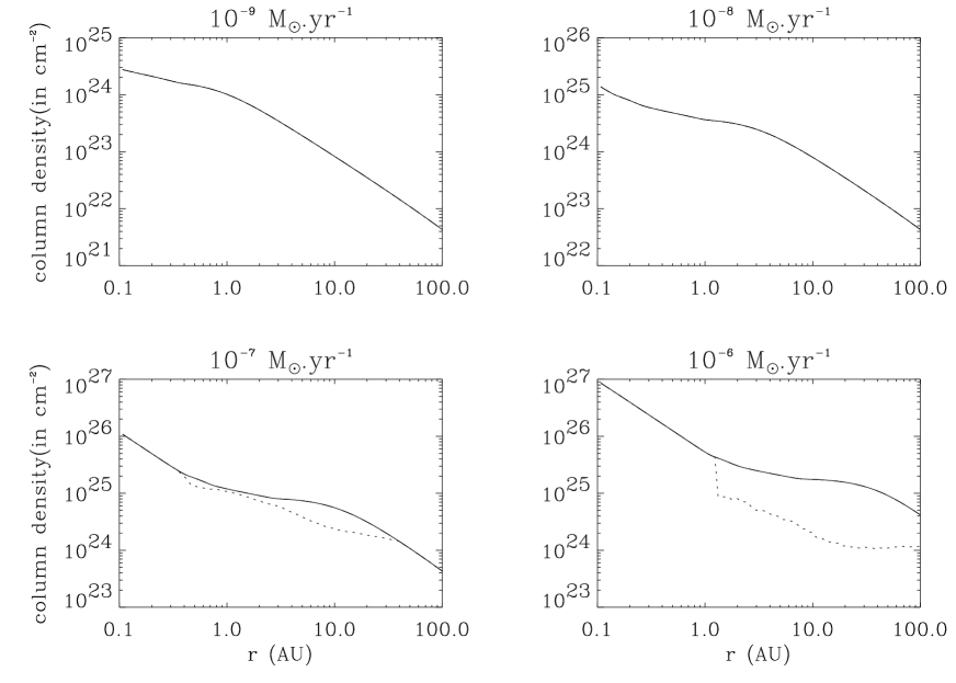
Figure 2: Column density, in cm^-2, of the whole disk (solid lines) and of the active zone for $Re_{M,{\rm crit}}=100$ (dotted lines). Here $x_{M}=0$, $\alpha=0.1$ and $\dot{M}=10^{-9}$ (upper left panel), $10^{-8}$ (upper right panel), $10^{-7}$ (lower left panel) and $10^{-6}$ M_⊙ yr^-1 (lower right panel). When the curve representing the active zone coincides with that representing the whole disk, then the whole disk is active. This is the case for $\dot{M}=10^{-9}$ and $10^{-8}$ M_⊙ yr^-1 when $Re_{M,{\rm crit}}=100$, and for all the values of $\dot{M}$ when $Re_{M,{\rm crit}}=1$.

In Figures 2–6, we plot the total column density, and that of the active layer, for different disk models: $\alpha=0.1$ (fig. 2 and 3), $10^{-2}$ (fig. 4 and 5) and $10^{-3}$ (fig. 6 and 7): $\dot{M}$ varies between $10^{-9}$–$10^{-6}$ M_⊙ yr^-1. Cases with $\alpha=10^{-2}$ and $\dot{M}=10^{-6}$ M_⊙ yr^-1 and $\alpha=10^{-3}$ and $\dot{M}\geq 10^{-7}$ M_⊙ yr^-1 have not been considered, as they give disk masses larger than that of the central star. Note that $x_{M}=0$ in figures 2, 4 and 6, whereas $x_{M}$ is finite in figures 3 and 5. In all figures, the X–ray luminosity and temperature are $L_{X}=10^{30}$ erg s^-1 and $kT_{X}=3$ keV respectively. When the entire disk is found to be active, a single curve is shown; otherwise, the difference between the two curves indicates the column density of the dead layer.

In table 1, we summarize the dead zone properties for the different models considered. The quantity $x_{M,{\rm min}}$ is the value of $x_{M}$ above which the dead zone disappears, and $r_{max}$ is the radius at which the vertical column density of the dead zone is largest. The final column is the percentage of the vertical column density occupied by the dead zone at $r=r_{max}$. Note that if $Re_{M,crit}=1$, $\alpha=0.1$ disks are all active throughout their entire extent, as are $\alpha=10^{-2}$ disks with $\dot{M}\leq 10^{-8}$ M_⊙ yr^-1. If one raises $Re_{M,crit}$ to 100, $\alpha=0.1$ disks are still magnetically active everywhere, when $\dot{M}\leq 10^{-8}$ M_⊙ yr^-1. As $\alpha$ increases, the disk surface density decreases at fixed $\dot{M}$, and the active zone increases in vertical extent.

Figures 3, 5, and 7 show that as $x_{M}$ increases, the dead zone shrinks both radially (with its outer edge moving inwards), and vertically. Its inner edge does not move outwards, because it is located at the radius at which the temperature drops below the level needed for thermal ionization to be effective, which is independent of $x_{M}$. For a given $\alpha$, this radius increases with $\dot{M}$, as the disk becomes hotter. Similarly, this radius increases when $\alpha$ decreases for $\dot{M}$ fixed.

The existence of a local maximum in the column density of the active layer at $r=r_{max}$ is easily understood. The $\alpha$–disk models have an almost uniform surface mass density over a broad radial range that depends on $\dot{M}$ and $\alpha$ (see fig. 1). As we move away from the star remaining in this region, the X–ray flux decreases because of simple geometrical dilution. Since the column density along the path of the photons stay about the same, the active layer becomes thinner. It starts to thicken only when the surface mass density in the disk begins to drop.

Table 1 gives the value of $x_{M}$ above which the disk is completely active. This should be compared with the cosmic abundance of the metal atoms present in a disk, which is $2\times 10^{-6}$ for Na and $3\times 10^{-5}$ for Mg (Anders & Grevesse 1989, Boss 1996). When $Re_{M,{\rm crit}}=100$ and for a disk model with $\alpha=10^{-2}$ and $\dot{M}=10^{-8}$ M_⊙ yr^-1, we see that an abundance of only $10^{-6}$ or even $10^{-7}$ of cosmic (depending on the species) is needed for the disk to be active.

When $\alpha\leq 10^{-3}$, the disk is never fully active, even for large values of $x_{M}$. This is because the disk is now very massive (about 0.3 solar mass within 100 AU for $\dot{M}=10^{-8}$ M_⊙ yr^-1), and there is a zone in the disk where X–rays simply cannot penetrate. Increasing $x_{M}$ clearly cannot prevent this!

5 Evolution of a disk with a dead zone

The fate of the magnetically coupled upper disk layers is far from clear. This relatively low density region may emerge in the form of a disk wind; it is also possible that the layers will accrete. This is the assumption of Gammie (1996), but it awaits verification by MHD simulations of stratified, partially ionized disks.

Should it occur, layered accretion in a disk will not be steady (Gammie 1996). The regions of the disk where there is an inactive layer act like a bottleneck through which the accretion is slowed and where matter therefore accumulates. Here we investigate whether enough mass can accumulate to make the disk locally gravitationally unstable. Of course, our calculation is in some sense not self-consistent, since it is based upon the assumption that the disk structure is a constant $\alpha$ model which we then show cannot be maintained! However, our interest is limited to estimating the extent to which upper layer accretion can build up the column density of the inner disk to the point of gravitational collapse. For this purpose, the precise vertical structure is likely to be a correction of detail, not a fundamental change.

Armitage et al. (2001) have considered a disk embedded in a collapsing envelope, so that mass is continuously added to the disk at a rate larger than the accretion through the disk itself. This strongly favors the development of gravitational instabilities. Here, we are concerned with the later stages of disk evolution, when there is no longer any infall. The inner regions are then supplied only by material coming from further out in the disk plane.

In a fully turbulent disk, the surface mass density evolves with time according to the following equation (Balbus & Papaloizou 1999):

$$\frac{\partial\Sigma}{\partial t}=\frac{1}{r}\frac{\partial}{\partial r}\frac{1}{\left(r^{2}\Omega\right)^{\prime}}\frac{\partial}{\partial r}\left(\Sigma r^{2}\langle W\rangle\right),$$ (18)

where $W$ is the horizontal stress tensor per unit mass averaged over the azimuthal angle, $\langle W\rangle=\int\rho Wdz/\Sigma$ is the density–averaged of $W$ over the disk thickness and the prime denotes derivative with respect to radius. For an $\alpha$ disk model, $W$ is given by (Shakura & Sunyaev 1973):

$$W=\frac{3}{2}\alpha c_{s}^{2}$$ (19)

where $c_{s}$ is the sound speed. There is no source term in equation (18) as there is no infall onto the disk.

In a layered disk, the right–hand–side of equation (18) also gives the variation per unit time of the surface mass density of the active zone, $\Sigma_{a}$, provided we replace $\Sigma$ by $\Sigma_{a}$ and $\langle W\rangle$ by $\langle W\rangle_{a}$. (The notation $\langle X\rangle_{a}=\int_{a}\rho Xdz/\Sigma_{a}$; the integration is over the active zone). But on the left–hand–side, $\Sigma$ must be replaced by $\Sigma_{d}$, the surface density of the dead zone. This is because, at a given location in the disk, $\Sigma_{a}$ is fixed, and determined by the X–ray source. Therefore, the mass which is added or removed at some radius is actually added to or removed from the dead zone. The evolution of the disk, in the parts where there is a dead zone, is then formally described by the two equations:

$$\frac{\partial\Sigma_{a}}{\partial t} = 0,$$ (20)

$$\frac{\partial\Sigma_{d}}{\partial t} = \frac{1}{r}\frac{\partial}{\partial r}\frac{1}{\left(r^{2}\Omega\right)^{\prime}}\frac{\partial}{\partial r}\left(\Sigma_{a}r^{2}\langle W\rangle_{a}\right),$$ (21)

Note that if $\Sigma_{d}$ given by equation (21) becomes negative at some location, then it means the dead zone disappears, and equation (18) should be used instead to evolve $\Sigma$, which is indistinguishable from $\Sigma_{a}$. Since $\langle W\rangle_{a}$ does not vary with time in our models, $\Sigma_{d}$ given by equation (21) varies linearly with time.

We consider as initial conditions a particular disk model characterized by the parameter $\alpha$ and a uniform $\dot{M}$. For illustrative purposes, we chose $\dot{M}=10^{-8}$ M_⊙ yr^-1 and $\alpha=3\times 10^{-2}$ and $10^{-2}$. The total surface mass density of such a disk is shown in Figure 8, where we also display the Toomre parameter, $Q(r)=\Omega c_{s}/[\pi G\Sigma(r)]$, where $G$ is the gravitational constant. To get a lower limit for $Q$, we evaluate $c_{s}$ at the disk surface. Because mass is going to accumulate at some intermediate radii in the disk, $Q$ is going to decrease there. We now investigate whether it can decrease enough for gravitational instabilities to develop, i.e. for $Q$ to drop to values $\sim 1$. Note that for $\dot{M}=10^{-7}$ M_⊙ yr^-1 and $\alpha=10^{-2}$, the initial disk model is already gravitationally unstable beyond about 30 AU (the total mass enclosed in this radius being about 0.03 M_⊙), which is why we consider here a smaller value of $\dot{M}$.

We compute the extent of the disk dead zone for $Re_{M,{\rm crit}}=100$ and $x_{M}=0$ (see § 4). To discuss the evolution of the disk, we need to consider the accretion rate through the disk, which is obtained from (Lynden–Bell & Pringle 1974):

$$\dot{M}=\frac{2\pi}{\left(r^{2}\Omega\right)^{\prime}}\frac{\partial}{\partial r}\left(\Sigma_{a}r^{2}\langle W\rangle_{a}\right).$$ (22)

(The $a$ subscripts should be dropped in the absence of a dead zone.) Here, $\dot{M}$ does not change with time. In Figure 8 we plot $\dot{M}$ versus $r$ at the radii where there is a dead zone. We see that $\dot{M}$ has a minimum at some location $r_{0}$. For $r<r_{0}$, $\dot{M}$ decreases with radius in the active region of the disk. The mass initially within $r_{0}$ in the dead zone will thus gradually be accreted onto the star, and whatever mass arrives at $r_{0}$ will subsequently be accreted as well. On the other hand, $\dot{M}$ increases with radius beyond $r_{0}$ in the active layer. Thus, in this region mass accumulates in the dead zone according to:

$$\Sigma\equiv\Sigma_{a}+\Sigma_{d}=\frac{1}{2\pi r}\frac{d\dot{M}}{dr}\;t+\Sigma_{i},$$ (23)

where $\Sigma_{i}$ is the initial value of $\Sigma$ at $r$, and equations (21) and (22) have been used. The evolution of the $Q$ parameter is then obtained simply from

$$Q\Sigma={\rm constant,}$$ (24)

where the constant is simply the initial value of the product. For the models whose initial conditions are shown in Figure 8, $Q$ reaches values around unity first at a radius of a few AU after a time of $2\times 10^{7}$ years. This is longer by about an order of magnitude than the disk lifetime inferred from observations (Haisch, Lada & Lada 2001). Note that this timescale is set by the largest value of $\Sigma$ reached at the end of the evolution and is thus insensitive to the starting conditions. A simple combination of layered accretion and gravitational instability does not appear to be sufficient to truncate our fiducial disk’s lifetime rapidly enough.

6 Discussion and conclusion

We have calculated a model for the ionization fraction of an $\alpha$–type disk, taking into account the full vertical structure of the disk. In common with other investigations (Gammie 1996, Glassgold et al. 1997), we have not included grain physics in our ionization model, which is an important limitation. Both the extent and the thickness of the dead zone depend sensitively on the parameters of the disk model, the gas accretion rate $\dot{M}$ and $\alpha$. For a critical Reynolds number of 100 and parameters believed to be typical of protostellar disks, the dead zone is found to extend from a fraction of an AU to 10–100 AU. For $\dot{M}=10^{-8}$ M_⊙ yr^-1 and $\alpha=10^{-2}$ for instance, the dead zone extends from 0.2 to 100 AU. For comparison, Igea & Glassgold (1999), who used a smaller value of $Re_{M,{\rm crit}}$, calculated that the dead zone extended to about 5 AU. (Also, since in this model the mass is more centrally condensed than in ours, the dead zone at 1 AU occupies a larger fraction of the disk vertical column density.) But for $\alpha=0.1$ and $\dot{M}<10^{-7}$ M_⊙ yr^-1, the disk can be magnetically coupled over its full extent. This is because the surface mass density is low in this case. Models with $\alpha=10^{-3}$ have a very large and thick dead zone. When $Re_{M,{\rm crit}}=1$, we have found that the dead zone is dramatically reduced or even disappears. Clearly, uncertainty in the input parameters profoundly influences the extent of magnetic coupling in protostellar disks, and full coupling to the field in some stages of disk evolution currently remains a possibility.

We have found that the characteristics of the dead zone are ultra–sensitive to the presence of heavy metal atoms in the disk. This is because the metal atoms are rapidly charged by molecular ions and recombine comparatively slowly. Molecular dissociative recombination is otherwise very rapid. For $\alpha=10^{-2}$ and $\dot{M}=10^{-8}$ M_⊙ yr^-1 for instance, an abundance of only $10^{-6}$–$10^{-7}$ of cosmic is all that is needed in our model for disk to be completely active, even when $Re_{M,{\rm crit}}=100$.

The density of metal atoms depends on the rate at which they are captured by grains and the rate at which they are liberated when an X–ray hits a grain. (Cosmic rays, which have been ignored here, may be important for this process.) The resulting density is very insensitive to the amount of dust present. If we assume that $\sigma_{rad}\sim\sigma_{cap}$ in equation (6), then $n_{M}=\epsilon L_{X}/(4\pi r^{2}v_{th}kT_{X})$ at the distance $r$ from the star, where $\epsilon$ is an efficiency factor (equal to the ratio of the quantum yield to the sticking probablity which were introduced in eq. [6]). With $L_{X}$ and $kT_{X}$ in the range $10^{29}$–$10^{31}$ erg s^-1 and 1–5 keV, respectively, $v_{th}\sim 1$ km s^-1, $\epsilon\sim 10^{-6}$ (Bringa 2001, private communication), we get a maximum value for $n_{M}$ which is about 200 cm^-3 at $r=1$ AU. For our fiducial values $\dot{M}=10^{-8}$ M_⊙ yr^-1 and $\alpha=10^{-2}$, the number density near the disk midplane at 1 AU is about $n=6\times 10^{13}$ cm^-3. The maximum value of the relative density of metal atoms is therefore $\sim 10^{-12}$, some $10^{-7}$–$10^{-6}$ of the cosmic abundance. This crude estimate shows that the density of metal atoms needed for magnetic coupling is within range reached, independently of the number of grains present. The presence of grains would certainly affect the ionization fraction. This is difficult to evaluate in a protostellar environment dominated by X-rays, and we have not attempted the calculation in this work. But it is important to note that the value of $n_{M}$ does not depend on the density of grains. It remains unchanged even in a disk where almost all the grains have sedimented toward the midplane. This is likely to be the situation in the later stages of disk evolution, as the sedimentation timescale for micron–size (or larger) grains is short (Nakagawa, Nakazawa & Hayashi 1981). Grain sedimentation and growth cause characteristic changes to the radiative spectral energy distribution. Such changes are in fact observed, though other interpretations cannot at present be ruled out (e.g., Beckwith, Henning & Nakagawa 2000).

Sano et al. (2000) investigated a finite density of metal atoms in a calculation of disk ionization (in their model produced by cosmic rays and radioactivity), together with the electrons–grains and ions–grains reactions. However, they assumed that the fraction of metal atoms in the gas phase was rather high, equal to $2\times 10^{-2}$. In their model, the relative abundance of metal atoms is therefore around $10^{-6}$ (they used a cosmic abundance of about $8\times 10^{-5}$ for the refractory heavy elements), several orders of magnitude higher than what we consider here. Their conclusion that the disk is almost completely turbulent when grains are sufficiently depleted depends very much upon this assumption.

Finally, we have estimated the evolutionary timescale against gravitational collapse of an $\alpha$ disk with a dead zone. In our fiducial model, we find that $\sim 10^{-3}$ M_⊙ accumulates between 2 and 20 AU, in regions of low optical depth at millimeter wavelengths. This would be easily detectable. The disk persists beyond $10^{7}$ years, an order of magnitude in excess of observational constraints. These results are rather robust. The difficulty suggests that a more elaborate model of the dead zone is required, or that disks are more ionized than our model indicates, or more broadly that simple layered accretion models may not be capturing the essential dynamics of disk accretion. A deeper understanding of disk ionization physics clearly is essential for further progress in this domain of star formation theory.

$Re_{M,{\rm crit}}$	$\alpha$	$\dot{M}$	$x_{M,{\rm min}}$	Inner radius	Outer radius	$r_{max}$	Column density
		(M⊙ yr-1)		(AU)	(AU)	(AU)
1	$10^{-2}$	$10^{-7}$	$10^{-17}$	5	60	20	50%
…	$10^{-3}$	$10^{-9}$	$10^{-16}$	2	30	5	65%
…	…	$10^{-8}$	$10^{-13}$	0.5	$\simeq 100$	10	90%
100	0.1	$10^{-7}$	$10^{-14}$	0.4	30	10	55%
…	…	$10^{-6}$	$10^{-13}$	1	$>100$	20	95%
…	$10^{-2}$	$10^{-9}$	$10^{-13}$	$<0.1$	20	2	70%
…	…	$10^{-8}$	$10^{-12}$	0.2	$\simeq 100$	6	90%
…	…	$10^{-7}$	$10^{-10}$	0.7	$>100$	20	98%
…	$10^{-3}$	$10^{-9}$		$<0.1$	$>100$	5	98%
…	…	$10^{-8}$		0.4	$>100$	10	99.9%

Table 1: Characteristics of the dead zone. Column 1 contains $Re_{M,{\rm crit}}$. In columns 2 and 3 are listed the parameters which characterized the disk, i.e. $\alpha$ and $\dot{M}$ in M_⊙ yr^-1. Column 4 contains $x_{M,{\rm min}}$, which is the value of $x_{M}$ above which there is no dead zone. The following columns contain the parameters which describe the dead zone for $x_{M}=0$: its inner radius (which is actually insensitive to $x_{M}$), its outer radius, the radius $r_{max}$ at which its vertical column density is maximum, and the percentage of the vertical column density it occupies at this radius. For $Re_{M,{\rm crit}}=1$, disks with $\alpha=0.1$ are completely active for all the values of $\dot{M}$, as are disks with $\alpha=10^{-2}$ and $\dot{M}\leq 10^{-8}$ M_⊙ yr^-1. For $Re_{M,{\rm crit}}=100$, disks with $\alpha=0.1$ and $\dot{M}\leq 10^{-8}$ M_⊙ yr^-1 are also completely active. For $Re_{M,{\rm crit}}=100$ and $\alpha=10^{-3}$, there is a dead zone for all the values of $x_{M}$.

Figure 1: Shown is the midplane temperature $T_{m}$ in K (left panel) and the surface mass density $\Sigma$ in g cm^-2 (right panel) vs. $r$ in AU for $\dot{M}=10^{-8}$ M_⊙ yr^-1 and $\alpha=10^{-3}$ (solid lines), $10^{-2}$ (dotted lines) and 0.1 (dashed lines). For comparison, the model used by Igea & Glassgold (1997) is also displayed (dotted–dashed lines).

Figure 3: Same as Fig. 2 but for $x_{M}\neq 0$. On each panel, the column density of the active zone is represented for $x_{M}=10^{-16}$ (dotted-dashed lines), $10^{-15}$ (dashed lines) and $10^{-14}$ (dotted lines). For $\dot{M}=10^{-9}$ and $10^{-8}$ M_⊙ yr^-1, the whole disk is active for all these values of $x_{M}$. For $\dot{M}=10^{-7}$ M_⊙ yr^-1, the whole disk is active for $x_{M}>10^{-15}$.

Figure 4: Same as Fig. 2 but for $\alpha=10^{-2}$ and for both $Re_{M,{\rm crit}}=100$ (dotted lines) and $Re_{M,{\rm crit}}=1$ (dashed lines). The case corresponding to $\dot{M}=10^{-6}$ M_⊙ yr^-1 has not been included as it gives a disk mass unrealistically large. Here, the whole disk is active when $Re_{M,{\rm crit}}=1$ only for $\dot{M}=10^{-9}$ and $10^{-8}$ M_⊙ yr^-1.

Figure 5: Same as Fig. 3 ($Re_{M,{\rm crit}}=100$) but for $\alpha=10^{-2}$ and for different values of $x_{M}$. On each panel, the column density of the active zone is represented for $x_{M}=10^{-13}$ (dotted-dashed lines), $10^{-12}$ (dashed lines) and $10^{-11}$ (dotted lines). The case corresponding to $\dot{M}=10^{-6}$ M_⊙ yr^-1 has not been included as it gives a disk mass unrealistically large. For $\dot{M}=10^{-9}$, $10^{-8}$ and $10^{-7}$ M_⊙ yr^-1, the whole disk is active for $x_{M}>10^{-13}$, $x_{M}>10^{-12}$ and $x_{M}>10^{-11}$, respectively.

Figure 6: Same as Fig. 4 but for $\alpha=10^{-3}$. Cases with $\dot{M}=10^{-7}$ and $10^{-6}$ M_⊙ yr^-1 have not been included as they give a disk mass unrealistically large.

Figure 7: Same as Fig. 3 ($Re_{M,{\rm crit}}=100$) but for $\alpha=10^{-3}$ and for different values of $x_{M}$. On each panel, the column density of the active zone is represented for $x_{M}=10^{-15}$ (dotted-dashed lines), $10^{-12}$ (dashed lines) and $10^{-9}$ (dotted lines). Cases with $\dot{M}=10^{-7}$ and $10^{-6}$ M_⊙ yr^-1 have not been included as they give a disk mass unrealistically large. Here the dead zone never disappears even for large values of $x_{M}$, and its extent does not vary with $x_{M}$ once $x_{M}\geq 10^{-9}$.

Figure 8: Initial conditions for the disk evolution. We consider a disk with $\dot{M}=10^{-8}$ M_⊙ yr^-1 and $\alpha=10^{-2}$ (solid lines) and $3\times 10^{-2}$ (dotted lines). Shown are the accretion rate $\dot{M}$ through the active layer of the disk in M_⊙ yr^-1 (upper left panel), the total surface mass density $\Sigma$ in g cm^-2 (upper right panel) and the Toomre $Q$ parameter (lower left panel) vs. $r$ in AU. Because $\dot{M}$ increases with $r$ beyond some radius, mass is going to accumulate in the dead zone at some intermediate radii during the disk evolution, and $Q$ is going decrease there. However, it does not reach the limit for gravitational instabilities within the disk lifetime.

References

- [1989] Anders E., & Grevesse N., 1989, Geochim. Cosmochim. Acta , 53, 197
- [2001] Armitage P.J., Livio M., & Pringle J.E., 2001, MNRAS, in press (astro-ph/0101253)
- [2000] Balbus S. A., & Hawley J.F., 2000, in From Dust to Terrestrial Planets, eds. W. Benz, R. Kallenbach & G.W. Lugmair, ISSI Space Sciences Series 9, Kluwer, p. 39
- [2001] Balbus S. A., & Terquem C., 2001, ApJ, 552, 235
- [2000] Beckwith S.V.W., Henning T., & Nakagawa Y. 2000, In Protostars & Planets IV, eds. V. Mannings, A.P. Boss & S.S. Russel, University of Arizona Press, Tucson, p. 533
- [1994] Bell K.R., & Lin D.N.C., 1994, ApJ, 427, 987
- [1994] Blaes O.M., & Balbus S.A., 1994, ApJ, 421, 163
- [1996] Boss A. P., 1996, ApJ, 469, 906
- [1996] Carkner L., Feigelson E.D., Koyama K., Montmerle T., & Reid I.N., 1996, ApJ, 464, 286
- [1995] Casanova, S., Montmerle, T., Feigelson, E. D., André, P. 1995, ApJ, 439, 752
- [1978] Consolmagno, G. J., Jokipii, J. R., 1978, Moon and Planets, 19, 253
- [2000] Fleming T. P., Stone J. M., & Hawley J. F., 2000, ApJ, 530, 464
- [1996] Gammie C.F., 1996, ApJ, 457, 355
- [1999] Gammie C.F., 1999, in Astrophysical Discs, eds. J.A. Sellwood & J. Goodman, ASP Conf. Series, 160, p. 122
- [1997] Glassgold A.E., Najita J., & Igea J., 1997, ApJ, 480, 344
- [2000] Glassgold A.E., Feigelson E. D., & Montmerle T. 2000, In Protostars & Planets IV, eds. V. Mannings, A.P. Boss & S.S. Russel, University of Arizona Press, Tucson, p. 429
- [2001] Haisch K. E., Jr., Lada E. A., & Lada C. J., 2001, ApJ, 553, L153
- [1985] Hayashi C., Nakazawa K., & Nakagawa Y., 1985, In Protostars & Planets II, eds. D.C. Black & M.S. Mathews, University of Arizona Press, Tucson, p. 1100
- [1999] Igea J., & Glassgold A. E., 1999, ApJ, 518, 848
- [1994] Koyama K., Maeda M., Ozaki M., Ueno S., Kamata Y., Tawara Y., Skinner S., & Yamauchi S., 1994, PASJ, 46, L125
- [Lynden] Lynden–Bell D., & Pringle J.E., 1974, MNRAS, 168, 60
- [1997] Millar T. J., Farquhar P. R. A., & Willacy K., 1997, A&AS, 121, 139
- [1981] Nakagawa Y., Nakazawa K., & Hayashi C. 1981, Icarus, 45, 517
- [1974] Oppenheimer M., & Dalgarno A., 1974, ApJ, 192, 29
- [1999] Papaloizou J.C.B., Terquem C., 1999, ApJ, 521, 823
- [1960] Parker E. N., 1960, ApJ, 132, 821
- [2000] Sano T., Miyama S. M., Umebayashi T., & Nakano T. 2000, ApJ, 543, 486
- [1973] Shakura N.I., & Sunyaev R.A., 1973, A&A, 24, 337
- [1992] Stepinski, T. F., 1992, Icarus, 97, 130
- [1999] Wardle M., 1999, MNRAS, 307, 849