An inverse Compton scattering (ICS) model of pulsar emission: II. frequency behavior of pulse profiles

Abstract

The shapes of pulse profiles, especially their variations with respect to observing frequencies, are very important to understand emission mechanisms of pulsars, while no previous attempt has been made in interpreting the complicated phenomenology. In this paper, we present theoretical simulations for the integrated pulse profiles and their frequency evolution within the framework of the inverse Compton scattering (ICS) model proposed by Qiao (1988) and Qiao & Lin (1998). Using the phase positions of the pulse components predicted by the “beam-frequency figure” of the ICS model, we present Gaussian fits to the multi-frequency pulse profiles for some pulsars. It is shown that the model can reproduce various types of the frequency evolution behaviors of pulse profiles observed.

1 Introduction

A wealth of observational data on radio pulsars has been collected since their discovery (for a review, see Lyne & Graham-Smith 1998). In history, understanding the nature of pulsar radio emission have been developed along two lines. On the one hand, the characteristics of pulsar pulse profiles have been studied empirically aiming at an understanding towards the emission beams. On the other hand, various plasma instabilities have been extensively studied motivated to find the right coherent mechanism to interpret the extremely high brightness temperatures observed. After more than 30 years, consensus on either of these two issues is yet fully achieved.

Diverse conclusions are reached after the various attempts in investigating pulsar radio emission beam shapes. Rankin (1983; 1993) proposed that the emission beam is composed of two distinct types of emission components, which are known as the core emission component near the center and the (two) conal components surrounding the core. Lyne & Manchester (1988) confirmed the different properties of core and conal emission, but suggested that the observations are better described by a gradual change in emission characteristics from the core or axial region to the outer edge emission beam, and that the pulsar radio beam is patchy, rather than a core plus two cones. The debate between the “core-cone” beam picture and the “patchy” beam picture has been persisting ever since (e.g. Gil & Krawczyk 1996; Mitra & Deshpande 1999; Han & Manchester 2001; Gangadhara & Gupta 2001, among others). It is possible that the real pulsar emission beam is the convolution of a “patchy” source function and a “window” function (Manchester 1995), which may itself be composed of a central core component plus one or more nested “conal” components. Despite of the discrepancy on the pulsar emission beam shapes, a wealth of multi-frequency observational data has been accumulated recently (e.g. Kramer et al. 1994; Gould & Lyne 1998; Kuzmin et al. 1998). The great varieties of the pulse profiles as well as their frequency evolution suggest the complexity of the pulsar beam patterns. For example, in some pulsars some wing (conal) components emerge at higher frequencies (e.g. PSR 1933+16, Sieber et al 1975), while in some other pulsars certain components disappear as the observational frequency evolves (e.g. PSR 1237+25, Phillips & Wolszczan 1992). The phase separation between various components also vary with frequency. All these provide invaluable information about the pulsar emission beams, and put important constraints on any theoretical model.

On the theoretical aspect, owing to the extreme environment within the pulsar inner magnetospheres (strong magnetic fields and electron-positron plasma), the identification of the pulsar radio emission mechanism has been a formidable task. More than ten radio emission models have been proposed. Among these, most models mainly focus on the condition for developing the instability which gives rise to coherent emission (Melrose 1992 for a review). Though theoretically rigorous, most of these models are either not well-modeled to be compared with the wealth of the observational data, or obviously conflict with the observations. The latest discussions include relativistic plasma emission (Melrose & Gedalin 1999), plasma maser (Lyutikov, Blandford & Machabeli 1999), spark-associated solitons (Gil & Sendyk 2000; Melikidze, Gil & Pataraya 2000), and inverse Compton scattering (Qiao & Lin 1998, hereafter Paper 1; Xu et al. 2000). Melrose (2000) argued that there is now a preferred pulsar emission mechanism which involves beam-driven Langmuir turbulence, based on the fact that such an instability involves a frequency $\nu_{\rm GJ}$ which is $\propto n_{\rm GJ}^{1/2}\propto B^{1/2}P^{-1/2}$ (see also eq.(2)), and is insensitive to the environments of either a normal pulsar or a millisecond pulsar. However, he pointed out a severe difficulty of the mechanism, i.e., the characteristic emission frequency is far too high compared to the observed frequency unless some non-standard plasma condition is introduced (see also Melrose & Gedalin 1999). Some efforts in comparing the model predictions with the observational data have been made within the maser model and the soliton model. However, it remains unclear whether the above-mentioned variaties of the frequency-evolution of the pulse profile patterns could be interpreted within these models. As far as we know, no attempt has been made in understanding the broad-band pulse profiles within the framework of other models, except the work by Sieber (1997) how considered a geometrical effect. The aim of the present paper is to carry out a simulation of the various frequency evolution patterns of pulsar integrated pulse profiles over a wide frequency range, within the framework of the inverse Compton scattering (hereafter ICS) model.

The arrangement of this paper is as follows. In §2, we review the basic picture of the ICS model, including a discussion of an important assumption made in the model. We then focus on a main theoretical result of the ICS model, i.e., the so-called “beam-frequency figure”, on which the later simulations rely. In §3, we present some multi-frequency pulse profile simulations for some typical pulsars of various types, using a Gaussian-fit according to the pulsar phase predictions made from the beam-frequency figure, and show how the model can reproduce various multi-frequency observational data. Our results are summarized in §4 with some discussions.

2 The ICS model and the “beam-frequency figure”

The basic picture of the ICS model is (Qiao 1988; Paper 1): a low-frequency electromagnetic wave is assumed to be excited near the pulsar polar cap region by the periodic breakdown of the inner gap (Ruderman & Sutherland 1975), and to propagate outwards in the open field line area up to some limited heights of interest. These low energy photons are inverse Compton scattered by the secondary particles produced in the pair cascades, and the up-scattered radio photons just provide the observed radio emission from the pulsar. Recent detailed polar cap “mapping” by Deshpande & Rankin (1999) indicates that the periodic storm induced by the gap breakdown is indeed happenning at least in some pulsars, which paves a solid observation foundation for the ICS model. It is then natural to expect the formation of a low frequency electromagnetic wave with the characteristic frequency $\nu_{0}\sim c/h\sim 10^{6}-10^{7}{\rm Hz}$ and its harmonics, where $c$ is the speed of light and $h$ is the gap height. The secondary pairs streaming out from the polar cap cascade with typical energy $\gamma=1/\sqrt{1-\beta^{2}}\sim 10^{3}$ will scatter these low frequency waves, and the up-scattered frequency reads (for $B\ll B_{q}=4.414\times 10^{13}$Gauss)

$$\nu\simeq 2\gamma^{2}\nu_{0}(1-\beta\cos\theta_{i}),$$ (1)

where $\theta_{i}$ is the incident angle (the angle between the direction of the particle and the incoming photons) of the scattering. Given a typical near-surface value of $(1-\beta\cos\theta_{i})\sim 10^{-3}$, one has $\nu\sim 10^{9}{\rm Hz}\gamma_{3}^{2}\nu_{0,6}$, which is the typical frequency of the pulsar radio emission. This makes ICS a plausible candidate for the pulsar radio emission mechanism. An important potential problem is the propagation of the low frequency wave in the pulsar magnetosphere. It is commonly believed that copious secondary pairs are produced at the upper boundary of the inner gap with a number density $n=\zeta n_{\rm GJ}$, where $\zeta\sim 10^{3}-10^{4}$ is the multiplicity (e.g. Daugherty & Harding 1982), and $n_{\rm GJ}\sim\Omega B/2\pi ec\sim 7\times 10^{10}\leavevmode\nobreak\ {\rm cm^{-3}}B_{12}/P$ is the Goldreich-Julian number density. The plasma frequency of this pair plasma is then

$$\omega_{p}=\left({4\pi ne^{2}\over m_{e}\gamma}\right)^{1/2}=1.5\times 10^{10}\left({\zeta_{3}B_{12}\over P\gamma_{3}}\right)^{1/2}\leavevmode\nobreak\ {\rm s^{-1}},$$ (2)

where $B_{12}$ is the local magnetic field strength in unit of $10^{12}$ G, and $P$ is the rotation period of the pulsar. Near the surface, this frequency is clearly much higher than $\nu_{0}$, which means that the low frequency wave excited by the gap breakdown may not be able to propagate. In fact, such waves are not detected, so that they must have been damped within the pulsar magnetosphere. However, it is still possible that the low frequency wave may propagate within the inner magnetosphere and be inverse Compton scattered before being damped. Strictly speaking, the argument that the low-frequency wave can not propagate only holds when the magnetosphere above the upper boundary of the gap is filled with the pair plasma. This might be the situation if the inner gap has a stationary pair formation front, which is the case of the stable space-charge-limited flow accelerator (e.g. Arons & Scharlemann 1979). In the breakdown picture we have assumed here (Ruderman & Sutherland 1975; Deshpande & Rankin 1999), the pair plasma is ejected in clumps, followed after each “sparking” process. This leaves many spaces between the adjacent plasma clouds with much less dense plasma so that the low frequency wave may propagate as if in vacuum. The plasma clumps will not spread until reaching the height

$$h_{sp}\sim\gamma^{2}h\sim 10^{9}\leavevmode\nobreak\ {\rm cm}\gamma_{3}^{2}h_{3},$$ (3)

which is about 100 times of stellar radii, beyond which the fast plasma will catch up with slow plasma to form a nearly uniform plasma. Empirical pulsar theories usually indicate that pulsar emission region is below or around this altitude, which raises the possibility of interpreting radio emission in terms of the ICS mechanism presented here. A full description of the propagation of the electromagnetic wave in such a rather unsteady, clumpy plasma is a very difficult task, and was not explored by previous authors. Here (and also in all the previous papers on the ICS model) we will assume that the low frequency wave may propagate to the necessary height of interest (e.g. below $h_{sp}$, eq.(3)), while postpone a detailed analysis of the propagation problem in future works. Our aim is to investigate the possible consequence of this strong assumption, and compare the model results to the observational data.

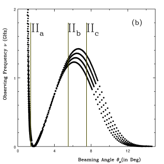
Figure 1: Two typical ”beam-frequency figures” in the ICS model. The observing frequency is plotted versus the so-called beaming angle, the angle between the radiation direction and the magnetic axis. (a) For Type I, the lines of a and b correspond to sub-types Ia and Ib. (b) For type II, the lines of a, b, and c correspond to the sub-types of IIa, IIb,and IIc.

If one naively regards that the low frequency wave propagates in the the near-surface polar cap region as if in vacuum, one can get an interesting picture of pulsar radio emission beam directly using eq.(1). Since the secondary pairs usually decelerates due to various energy loss mechanisms (e.g. Zhang, Qiao & Han 1997), one may usually assume

$$\gamma=\gamma_{0}\exp(-\xi\frac{r-R}{R}),$$ (4)

where $\gamma_{0}$ is the initial Lorentz factor of the particles, $R$ is the radius of of the neutron star, $r-R$ is the emission height from the neutron star surface, and $\xi$ reflects the scale factor of the deceleration. On the other hand, basic dipolar geometry (Fig.1 in Paper 1) indicates that the term $(1-\beta\cos\theta_{i})$ will first decrease with height, then increase sharply after passing the crossing point defined by $\theta_{i}=0$, and finally only increase mildly. The competition between this geometric effect and the deceleration effect then results in a drop-rise-drop pattern for the emission frequency as the height increases. Since the field opening angle increases with the height, the drop-rise-drop pattern also holds for the frequency-beaming angle plot. This is the so-called “beam-frequency figure” or the “beaming figure” of the ICS model, which is the starting point of the simulations in $\S 3$. Figure 1a,b are typical beam-frequency figures of the ICS model. Fixing an observation frequency $\nu$, there are three heights (and opening angles) where the emission with this frequency comes out. This naturally gives rise to a central core emission component and two conal components, meeting Rankin’s (1983) original proposal. One remark is that the three-component scheme is an average picture, which resembles Manchester’s (1995) “window” function. In a certain pulsar, some favored spots may generate more clumps and hence, more emission, so that the actual emission beam could be patchy within the three-component window.

In a beam-frequency figure, we can define the three branches as the “core branch”, the “inner conal branch” and the “outer conal branch”, respectively, as indicated in Fig.1. How many branches are observable also depends on the line-of-sight of the observer, which defines the minimum beam angle.

3 Frequency behaviour of the integrated pulse profiles

In this section, an important observational feature, i.e., the integrated pulse shape evolution with frequencies, will be investigated. The key points are how many components in a pulse profile exist and what positions of these components are, which can be retrieved from the “beam-frequency figures” as described above. Once this information is available, we then assume that the shape of each emission component is Gaussian, as has been widely adopted in many other studies (e.g. Kramer et al. 1994; Kuzmin et al. 1996; Wu et al. 1998). Since the height and the width of Gaussian function are hard to derive from the first principle, we take them as inputs to meet the observations. We can then finally get the integrated pulse profiles of a pulsar for various frequencies. In the following, we will show some simulation examples for several different types of the pulsar profiles and their frequency evolution. A preliminary consideration has been previously presented by Qiao (1992) and Liu & Qiao(1999).

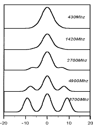
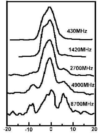
Figure 2: A simulation for the type Ia pulsar PSR B1933+16. $P=0.3587s$, the inclination angle $\alpha=45^{\circ}$, the impact angle $\beta=0$, $\gamma_{0}=3000$, $\xi=10^{-4}$. We compute the locations of the cones using the field line whose base is 0.8 of the polar cap radius. In the right column figure we present the observational data from Lyne & Manchester (1988) for 1420MHz, 2700MHz and 8700MHz, and from Sieber et al. (1975) for 430MHz and 4900MHz, for a closer comparison. Hereafter left columns represent the simulation results; while right columns are the multi-frequency observational results. The horizontal axis is the longitude (in degrees).

3.1 Core dominant pulsars

The scheme of this kind of pulsars is that only the core branch and the inner conal branch exist in the pulsar beam. This usually takes place in the short period pulsars whose polar caps are larger (e.g. Fig.4 and Fig.6b in Paper I) than those of the long period pulsars. The missing of the outer conal branch is either due to that the deceleration of the pairs is not important or due to that the low frequency wave may not propagate to higher altitudes. As the impact angle gradually increases, pulsars of this kind can be further grouped into two sub-types.

Type Ia. Core-single to core-triple pulsars

Pulsars of this type have very small impact angles. They normally show single pulse profiles at low frequencies but become triple profiles at high frequencies when the line-of-sight starts to cut across the inner conal branch.

The multi-frequency observations of PSR B1933+16 (Sieber et al. 1975; Lyne & Machester 1988) show that it belongs to this type. Its profiles are single when observation frequencies are lower than 1.4 GHz, but become triple at higher frequencies. A simulation for PSR B1933+16 is presented in Fig.2. We can see the single-to-triple profile evolution with increasing frequency. Furthermore, the separation between the two “shoulders” of the triple profile gets wider at higher frequencies. Evidently the radius of the “inner” cone increases at higher frequencies, which is an important feature of the ICS model distinguished from the others (see Sect.3.2 of paper 1).

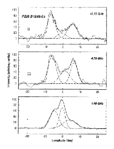
Figure 3: A simulation for the Type Ib pulsar PSR B1845-01. P=0.651 s, Model parameters: $\alpha=45^{\circ}$, $\beta=2.1^{\circ}$ is large enough that at higher frequencies the core component is almost disappearing. $\gamma_{0}=3000$, $\xi=10^{-4}$. The observations are from Kramer (1994).

Type Ib. Core-triple to conal-double pulsars

Pulsars of this type have larger impact angles than those of Type Ia. Though at low frequencies the pulsars show core-triple profiles, they will evolve to conal-double profiles at higher frequencies, when the lines-of-sight starts to miss the core branch. An example of this type is PSR B1845-01 (see Fig.3 and Kramer et al. 1994 for the relevant data). From both the ICS model and observations one can see several important characteristics of this kind of pulsars. These are: (1) The radius of the inner cone increases with the increasing observing frequency, which is different from that of the outer cone; (2) Owing to the line-of-sight effect the intensity of the central emission component decreases rapidly as the observing frequency increases. These characteristics are very different from those of any model involving curvature radiation. Another example of this type is PSR B1508+55 (Kuzmin et al. 1998; Sieber et al. 1975).

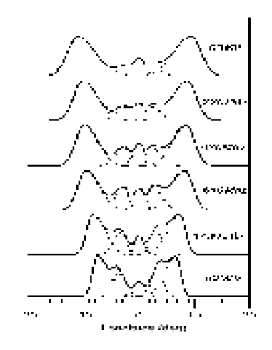
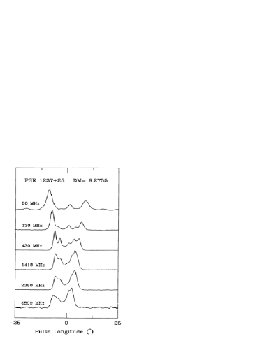
Figure 4: A simulation for the Type IIa pulsar PSR B1237+25. P=1.38 s, $\alpha=48.2^{\circ}$, $\beta=1^{\circ}$, $\gamma_{0}=4000$, and $\xi=0.02$. Note that the retardation effect is taken into consideration and the central component is off-centered. Observations are from Phillips & Wolszczan (1992).

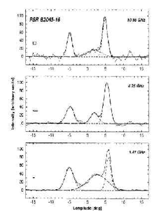
Figure 5: A simulation for the Type IIb pulsar PSR B2045-16. P=1.96 s, $\alpha=45^{\circ}$, $\beta=9^{\circ}$, $\gamma_{0}=5000$, and $\xi=0.002$. The observations follow Kramer (1994).

3.2 Conal dominant pulsars

The scheme of this kind of pulsars is that all three branches exist in the pulsar beam. This usually occurs in long period pulsars, mainly because the turning point in the beaming figure ($\theta_{i}=0$) gets shifted to lower altitudes due to the geometric effect. This would be the most common case. Pulsars in this scheme can be grouped into three sub-types as the impact angle gradually increases.

Type IIa Multi-component pulsars

Pulsars of this type have five components at most observing frequencies, since the small impact angle makes the line-of-sight cut through all the three branches. A very important feature is that according to the ICS model, the five pulse components will merge into three components at very low frequencies (see Fig.1b, line IIa in this paper). This has indeed been observed from some pulsars, e.g., PSR B1237+25 (see Phillips & Wolszczan 1992, noticing the three components at very low frequency of 50 MHz). It is worth emphasizing that the ICS model has the ability to interpret this important feature, which would be a challenge to most of other models. The simulation results for PSR B1237+25 are presented in Fig.4. Because three emission components are emitted at different heights, the retardation is important to perform a realistic simulation. In our simulation, such a retardation effect was taken into account to reproduce a peculiar observed feature of this pulsar, i.e., an off-centered central component closer to the trailing conal components.

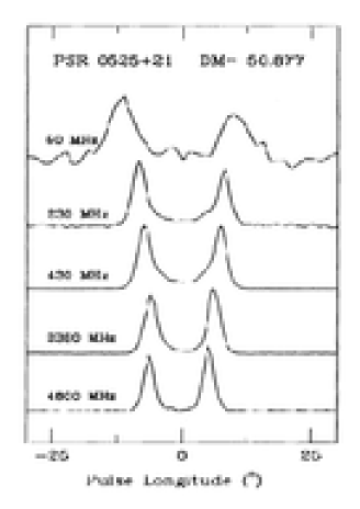
Figure 6: A simulation for the Type IIc pulsars PSR B0525+21. P=3.745 s, $\alpha=45^{\circ}$, $\beta=6^{\circ}$, $\gamma_{0}=5000$, and $\xi=0.002$. The observations are from Phillips & Wolszczan (1992).

Type IIb Conal triple pulsars

The impact angle is larger in this sub-type, so that at higher frequencies, the line-of-sight does not cut through the core branch. Thus pulsars show three components at low observing frequencies, then evolve to four components when frequency is higher, and finally merge to double pulse profiles at the highest frequency.

An example is PSR B2045-16 (e.g. Kramer et al. 1994), which we have simulated in Fig.5. The pulse profile is “triple” for this pulsar. The separation of the two outer components are wider at lower frequencies.

Type IIc Conal double pulsars

Pulsars of this type have the largest impact angle, so that only the outer conal branch is cut by the line-of-sight. The pulse profiles of this type are conal double at all observing frequencies, with the separation between the two components decreasing at higher frequencies. This is just the traditional radius-to-frequency mapping which has also been calculated in the curvature radiation picture. A typical one is PSR B0525+21 (Phillips & Wolszczan 1992), and we have simulated it in Fig.6.

Another situation of this type is that pulsars have single profiles at most of observing frequencies, but become double components at very low observing frequencies, an example of this kind may be PSR B0950+08 (e.g. Kuzmin et al. 1998).

4 Conclusions and discussions

1. Based on a simple ICS picture, we have simulated the frequency evolution of the pulsar integrated pulse profiles of several pulsars. It is worth mentioning that the observed evolution behavior is quite complicated, and there are many different kinds of evolutionary patterns. This would be a challenge to most presently discussed radio emission models. In this paper, we find a clear scheme to understand such a variety of the evolutionary styles within the ICS model. Different kinds of frequency evolution styles could be grouped into two basic categories, each of which may be grouped into some further sub-types according to the line-of-sight effect. Though there are some uncertainties due to the model assumption, the simulations presented here can give a first-order description of the pulsar profiles. The fundamental difference between the ICS and the curvature radiation mechanism is that the latter can only give hollow cones. Due to the monotonic beaming-frequency figure of curvature radiation, formation of the different emission components should be attributed to the multi-components of the sparking sources (e.g. Gil & Sendyk 2000). In the ICS model, one sparking source can naturally account for three emission components at different altitudes due to the special beaming figure (Fig.1).

2. As discussed in §2, we have introduced a strong assumption throughout the analysis, i.e., the gap sparking-induced low frequency electromagnetic wave can propagate up to a certain height and be scattered by the secondary pairs before being damped at higher altitudes. We have discussed that the strong unsteady pair process near the pulsar polar cap region may make this possible, although we concede that more rigorous and detailed justification about this assumption is desirable. Nevertheless, the naive picture introduced here seems to have the ability to reproduce various types of the pulsar integrated pulse profile patterns and their frequency evolution, which would be difficult for most of the other theoretically rigorous models. Another caveat about the propagation problem is that according to eq.(2), even the observed radio emission can not propagate near the surface, while observations show that at least some emission components (e.g. the core emission) may come from the surface (Rankin 1990). Some other ideas that may allow propagation of the low frequency wave include the radiation-pressure-induced plasma rarefication (Sincell & Coppi 1996) and the non-linear plasma effect (e.g. Chian & Kennel 1983).

3. Observationally, it has been argued that different emission components may come from different heights (e.g. Rankin 1990; 1993). More specifically, Rankin (1990) found that the profile widths of the core single pulsars are remarkably consistent with the prediction of a near-surface emission with dipolar field configuration, which hints that the core emission may come from the near polar cap region. If it is indeed so, then the ICS model gives a natural explanation of the near-surface core emission. All the other presently discussed models (Melrose 2000; Lyutikov et al. 1999; Melikidze et al. 2000) exclusively predict a much higher emission altitude for both the core and the conal emission components.

4. Our model calculations show that in order for the low frequency wave to be generated, pulsars should have oscillatory inner gaps. This is a natural expectation if the inner gap of a pulsar is vacuum-like (Ruderman & Sutherland 1975) rather than a steady space-charge-limited flow (Arons & Scharlemann 1979). In the conventional neutron star picture, this requires that the star is an “anti-parallel rotator”, i.e., $\Omega\cdot B<0$, with a large enough ion binding energy on the surface. If pulsars are born with random orientations of spin and magnetic axes, the present model would then only applies to one half of the neutron stars. If the space-charge-limited accelerator can somehow show an oscillatory behavior (e.g. Muslimov & Harding 1997), then our model can also apply to the other half of the neutron stars. Furthermore, if pulsars are strange quark stars with bare polar cap surfaces (e.g. Xu, Qiao & Zhang 1999), one expects a vacuum gap forming in both $\Omega\cdot B<0$ and $\Omega\cdot B>0$ configurations. Another caveat is that there might be more than one radio emission mechanisms operating in pulsars. For example, some young pulsars have an emission component with almost 100% linear polarization, very likely with a high-altitude wide cone configuration. This component may be due to some other reasons (e.g. the maser model by Lyutikov et al. 1999), and may be also produced by a steady space-charge-limited accelerator. Future broadband observations (radio, optical, X-ray, and $\gamma$-ray) from some pulsars may eventually reveal the geometric configurations for the emission components in various bands, and shed some lights on our understanding of the pulsar radio emission mechanisms.

- (1) Arons, J., & Scharlemann, E.T. 1979, ApJ, 231, 854
- (2) Chian, A. C.-L., & Kennel, C. F. 1983, Ap&SS, 97, 9
- (3) Daugherty, J. K., & Harding, A. K. 1982, ApJ, 252, 337
- (4) Deshpande, A.A., & Rankin, J.M. 1999, ApJ, 524, 1008
- (5) Gangadhara, R.T., & Gupta, Y. 2001, ApJ, in press (astro-ph/0103109)
- (6) Gil, J.A., & Krawczyk, A. 1996, MNRAS, 280, 143
- (7) Gil, J.A., & Sendyk, M. 2000, ApJ, 541, 351
- (8) Gould, D.M., & Lyne, A.G. 1998, MNRAS, 301, 235
- (9) Han, J.L., & Manchester, R.N., 2001, MNRAS 320, L35
- (10) Kramer M., 1994, A&A Suppl. Ser. 107, 527
- (11) Kuzmin, A.D. & Izvekova, V.A., 1996, Astronmy Letters, 22, 3, 394
- (12) Kuzmin, A.D., Izvekova, V.A., Shitov, Yu.P., Sieber, W., Jessner, A., Weilebinski, R., Lyne, A.G., & Smith, F.G. 1998, A&AS, 127, 355
- (13) Liu, J.F. & Qiao, G.J., 1999, Chinese Astronomy and Astrophysics, 23, 133
- (14) Lyne, A.G., & Manchester, R.N. 1988, MNRAS, 234, 477
- (15) Lyne, A.G., & Graham-Smith, F. 1998, Pulsar Astronomy (2rd ed.: Cambridge: Cambridge Univ. Press)
- (16) Lyutikov, M., Blandford, R.D., & Machabeli, G. 1999, MNRAS, 305, 338
- (17) Manchester, R.N. 1995, J. Astrophys. Astr. 16, 107
- (18) Melikidze, G.I., Gil, J.A., & Pataraya, A.D. 2000, ApJ, 544, 1081
- (19) Melrose, D.B., 1992, T.H. Hankins, J.M. Rankin, & J.A. Gil (eds) IAU Colloq. 128, The Magnetospheric Structure and Emission Mechanisms of Radio Pulsars(hereafter IAU Coll. 128), Zielona Gora, Poland: Pedagogical Univ. Press, 306
- (20) Melrose, D.B., 2000, ASP Conference Series, Vol.202, p.721
- (21) Melrose, D.B., & Gedalin, M. E., 1999, ApJ, 521, 351
- (22) Mitra D.,& Deshpande, A.A., 1999, A&A, 346,906
- (23) Muslimov, A., & Harding, A.K. 1997, ApJ, 485, 735
- (24) Phillips, J.A., & Wolszczan, A. 1992, ApJ, 385, 273
- (25) Qiao, G.J. 1988, Vistas in Astronomy, 31, 393
- (26) —–. 1992, IAU Coll. 128, p.239
- (27) Qiao, G.J., & Lin W.P. 1998, A&A, 333, 172 (Paper 1)
- (28) Rankin, J.M. 1983, ApJ, 274, 333
- (29) —–. 1990, 1990, ApJ, 352, 314
- (30) —–. 1993, ApJS, 85, 145
- (31) Ruderman, M.A.& Sutherland, P.G. 1975, ApJ, 196, 51
- (32) Sieber, W., Reinecke, R.,& Wielebiski, R. 1975, A&A, 38, 169
- (33) Sieber, W. 1997, A&A, 321, 519
- (34) Sincell, M. W., & Coppi, P. S. 1996, ApJ, 460, 163
- (35) Wu, X.J., Gao, X.Y., Rankin, J.M., Xu, W.& Malofeev, V.M., 1998, Astronomical Journal, 116,1984
- (36) Xu, R.X., Liu, J.F., Han, J.L., & Qiao, G.J. 2000, ApJ, 535, 354
- (37) Xu, R.X., QIao, G.J., & Zhang, B. 1999, ApJ, 522, L109
- (38) Zhang, B., & Qiao, G.J., & Han, J.L. 1997, ApJ, 491, 891