The HELLAS2XMM survey: I. The X-ray data and the Log(N)-Log(S)

Abstract

We present the first results from an XMM-Newton serendipitous medium-deep survey, which covers nearly three square degrees. We detect a total of 1022, 495 and 100 sources, down to minimum fluxes of about $5.9\times 10^{-16}$, $2.8\times 10^{-15}$ and $6.2\times 10^{-15}$ erg cm^-2 s^-1, in the 0.5-2, 2-10 and 4.5-10 keV band, respectively. In the soft band this is one of the largest samples available to date and surely the largest in the 2-10 keV band at our limiting X-ray flux. The measured Log(N)-Log(S) are found to be in good agreement with previous determinations. In the 0.5-2 keV band we detect a break at fluxes around $5\times 10^{-15}$ erg cm^-2 s^-1. In the harder bands, we fill in the gap at intermediate fluxes between deeper Chandra and XMM-Newton observations and shallower BeppoSAX and ASCA surveys.

1 Introduction

In the last decade it has become progressively clearer that the extragalactic X-ray background (XRB) originates from the superposition of many unresolved faint sources.
In the soft band (0.5-2 keV) ROSAT has resolved about 70%-80% of the XRB (Hasinger et al., 1998), meanwhile recent Chandra deep observations are resolving almost all the background (Mushotzky et al., 2000; Giacconi et al., 2001). The hard band (2-10 keV) XRB has been resolved at a 25%-30% level with BeppoSAX and ASCA surveys (Cagnoni, Della Ceca, & Maccacaro, 1998; Ueda et al., 1999; Giommi, Perri, & Fiore, 2000) and recently at more than 60% with Chandra (Mushotzky et al., 2000; Giacconi et al., 2001; Hornschemeier et al., 2001). Moreover, in the very hard band (5-10 keV) the fraction resolved by BeppoSAX is around 30% (Fiore et al., 1999; Comastri et al., 2001) and very recently in the XMM-Newton Lockman Hole deep pointing about 60% is reached (Hasinger et al., 2001).
The spectroscopic follow up of the objects making the XRB find predominantly Active Galactic Nuclei (AGN). In the soft band, where optical spectroscopy has reached a high degree of completeness, the predominant fraction is made by unabsorbed AGN (type-1 Seyferts and QSOs), with a small fraction of absorbed AGN (essentially type-2 Seyferts) (Bower et al., 1996; Schmidt et al., 1998; Zamorani et al., 1999). The fraction of absorbed type-2 AGN rises if we consider the spectroscopic identifications of hard X-ray sources in BeppoSAX, ASCA and Chandra surveys (La Franca et al., 2001; Fiore et al., 2001a; Akiyama et al., 2000; Della Ceca et al., 2000; Barger et al., 2001; Tozzi et al., 2001), although the optical follow up is far from being complete.
The X-ray and optical observations are consistent with current XRB synthesis models (Setti & Woltjer, 1989; Comastri et al., 1995; Gilli, Salvati, & Hasinger, 2001), which explain the hard XRB spectrum with an appropriate mixture of absorbed and unabsorbed AGN, by introducing the corresponding luminosity function and cosmological evolution. In this framework, Fabian & Iwasawa (1999) infer an absorption-corrected black hole mass density consistent with that estimated from direct optical and X-ray studies of nearby unobscured AGN. This result requires that most of the X-ray luminosity from AGN ($\sim 80\%$) is absorbed by surrounding gas and probably re-emitted in the infrared band.
However synthesis models are far from being unique, depending on a large number of hidden parameters. They require, in particular, the presence of a significant population of heavily obscured powerful quasars (type-2 QSOs). Type-2 QSOs have been revealed first by ASCA and BeppoSAX (Ohta et al., 1996; Vignati et al., 1999; Franceschini et al., 2000) and are starting to be discovered at high redshift by Chandra (Fabian et al., 2000; Norman et al., 2001). These objects are rare (so far, only a few type-2 QSOs are known), luminous and hard (heavily absorbed in the soft band). A good way of finding them is to perform surveys in the hard X-ray bands, covering large solid angles. The large throughput and effective area, particularly in the harder bands, make XMM-Newton currently the best satellite to perform hard X-ray surveys.
In this paper we present an XMM-Newton medium-deep survey covering nearly three square degrees, one of its main goals is to constrain the contribution of absorbed AGN to the XRB. We first overview the data preparation (Section 2) and the source detection (Section 3) procedures, describing then the survey characteristics (Section 4) and the first purely X-ray results we obtain from the Log(N)-Log(S) (Section 5). An extensive analysis of the X-ray broad-band properties of the sources and the optical follow-up of a hard X-ray selected sample will be the subjects of forthcoming papers (Baldi et al. in prep.)

2 Data preparation

The survey data are processed using the XMM-Newton Science Analysis System (XMM-SAS) v5.0.
Before processing, all the datasets have been supplied with the attitude of the satellite, which can be considered stable within one arcsecond during any given observation. Thus, a good calibration of the absolute celestial positions (within $2^{\prime\prime}-3^{\prime\prime}$) has been obtained from the pointing coordinates in the Attitude History Files (AHF). Standard XMM-SAS tasks $epproc$ and $emproc$ are used to linearize the pn and MOS camera event files.
The event files are cleaned up from two further effects, hot pixels and soft proton flares, both worsening data quality.
The hot and flickering pixel and the bad column phenomena, partly due to the electronics of the detectors, consist basically in the non-X-ray switching-on of some pixels during an observation and may cause spurious source detections. The majority of them are removed by the XMM-SAS; we localize the remaining using the IRAF task $cosmicrays$ and remove all the events matching their positions using the multipurpose XMM-SAS task $evselect$.
Soft proton flares are due to protons with energies less than a few hundred keV hitting the detector surface. These particles strongly enhance the background during an observation; for example $\sim 40\%$ of the long Lockman Hole observation was affected by them. The background enhancement forces us to completely reject these time intervals with the net effect of a substantial reduction of the good integration time. We locate flares analyzing the light curves at energies higher than 10 keV (in order to avoid contribution from real X-ray source variability), setting a threshold for good time intervals at 0.15 cts/s for each MOS unit and at 0.35 cts/s for the pn unit.

3 Source detection

The clean linearized event files are used to generate MOS1, MOS2 and pn images in four different bands: 0.5-2 keV, 2-10 keV, 2-4.5 keV and 4.5-10 keV. All the images are built up with a spatial binning of 4.35 arcseconds per pixel, roughly matching the physical binning of the pn images ($4^{\prime\prime}$ pixels) and a factor of about four larger than that of the MOS images ($1.1^{\prime\prime}$ pixels). In any case, the image binning does not worsen XMM-Newton spatial resolution, which depends almost exclusively from the point spread function (PSF).
A corresponding set of exposure maps is generated to account for spatial quantum efficiency, mirror vignetting and field of view of each instrument, running XMM-SAS task $eexpmap$. This task evaluates the above quantities assuming an event energy which corresponds to the mean of the energy boundaries. In the 2-10 keV band, which covers a wide range of energies, this may lead to inaccuracies in the estimate of these key quantities. Thus we create the 2-10 keV band exposure map as a weighted mean between the 2-4.5 keV and the 4.5-10 keV exposure maps, assuming an underlying power-law spectral model with photon index 1.7.
The excellent relative astrometry between the three cameras (within $1^{\prime\prime}$, well under the FWHM of the PSF) allows us to merge together the MOS and pn images in order to increase the signal-to-noise ratio of the sources and reach fainter X-ray fluxes; the corresponding exposure maps are merged too.
The source detection and characterization procedure applied to the image sets involves the creation of a background map, for each energy band. The first step is to run an XMM-SAS $eboxdetect$ local detection (in each band independently) to create a source list. Then XMM-SAS $esplinemap$ removes from the original merged image (within a radius of 1.5 times the FWHM of the PSF) all the sources in the list and creates a background map fitting the remaining (the so-called cheesed image) with a cubic spline. Unfortunately, even using the maximum number of spline nodes (20), the fit is not sufficiently flexible to reproduce the local variations of the background. Thus we correct the background map pixel by pixel, measuring the counts in the cheesed image ($cts_{ch}$) and in the background map itself ($cts_{bk}$), within three times the radius corresponding to an encircled energy fraction (EEF) of the PSF of $\alpha=0.68$ (hereafter $r_{0.68}$). We create a corrected background map by multiplying the original image by a correction factor which is the $cts_{ch}$ to $cts_{bk}$ ratio. After some tests, the radius of $3r_{0.68}$ has been considered a good compromise between taking too many or too few background fluctuations.
A preliminary $eboxdetect$ local mode detection run, performed simultaneously in each energy band, creates the list of candidate sources on which to carry out the characterization procedure.
Each candidate source is characterized within a radius $r_{0.68}$, evaluating the source counts $S$ and error $\sigma_{S}$ (using the formula of Gehrels, 1986) following the formulas:

$$S=\frac{cts_{img}-cts_{bkg}}{\alpha}\>,\>\>\>\>\>\>\>\>\>\>\sigma_{S}=\frac{1+\sqrt{cts_{img}+0.75}}{\alpha}\>,$$

where $cts_{img}$ are the counts (source + background) within $r_{0.68}$ in the image and $cts_{bkg}$ are the background counts in the same area in the background map. The count rate is then:

$$cr=\frac{S}{T_{MOS1}+T_{MOS2}+T_{pn}}\>,$$

where $T_{MOS1}$, $T_{MOS2}$ and $T_{pn}$ are the exposure times of the three instruments computed from the exposure maps.
The count rate-to-flux conversion factors are computed for each instrument using the latest response matrices and assuming a power-law spectral model with photon index 1.7 and galactic $N_{H}$. The total conversion factor $cf$ has been calculated using the exposure times for MOS1, MOS2 and pn, the conversion factors for the three instruments, $cf_{MOS1}$, $cf_{MOS2}$ and $cf_{pn}$, following the formula:

$$\frac{T_{tot}}{cf}=\frac{T_{MOS1}}{cf_{MOS1}}+\frac{T_{MOS2}}{cf_{MOS2}}+\frac{T_{pn}}{cf_{pn}}\>,$$

where $T_{tot}=(T_{MOS1}+T_{MOS2}+T_{pn}$). The source flux is straightforwardly:

$$F_{x}=cf\cdot cr\>.$$

For each source we compute $p$, the probability that counts originate from a background fluctuation, using Poisson’s formula:

$$\sum_{n=cts_{img}}^{\infty}e^{-cts_{bkg}}\frac{cts_{bkg}^{n}}{n!}>p\>;$$

we choose a threshold of $p=2\times 10^{-4}$ to decide whether to accept or not a detected source.

4 The survey

Our survey covers 15 XMM-Newton calibration and performance verification phase fields. The pointings and their characteristics are listed in Table 1. All fields are at high galactic latitude ($|bII|$ $>$ 27^o), in order to minimize contamination from galactic sources, have low galactic $N_{H}$ and at least 15 ksec of good integration time.
The sky coverage of the sample has been computed using the exposure maps of each instrument, the background map of the merged image and a model for the PSF. We adopt the off-axis angle dependent PSF model implemented in XMM-SAS $eboxdetect$ task.
At each image pixel $(x,y)$ we evaluate, within a radius $r_{0.68}$, the total background counts (from the background map). From these we calculate the minimum total counts (source + background) necessary for a source to be detected at a probability $p=2\times 10^{-4}$ (defined in Section 3). The mean exposure times for MOS1, MOS2 and pn, evaluated from the exposure maps within $r_{0.68}$, are used to compute the count rate $cr$. From the count rate-to-flux conversion factor $cf$ (computed as in Section 3) we build a flux limit map and straightforwardly calculate the sky coverage of a single field.
Summing the contribution from all fields we obtain the total sky coverage of the survey, which is plotted in Figure 1, in three different energy bands.

5 Log(N)-Log(S)

The cumulative Log(N)-Log(S) distribution for our survey has been computed by summing up the contribution of each source, weighted by the area in which the source could have been detected, following the formula:

$$N(>S)=\sum_{S_{i}>S}\frac{1}{\Omega_{i}},$$

where $N(>S)$ is the surface number density of sources with flux larger than $S$, $S_{i}$ is the flux of the $i$th source and $\Omega_{i}$ is the associated solid angle.
It is worth noting that XMM-Newton calibrations are not yet fully stable and systematic errors in the determination of the Log(N)-Log(S) could arise, for instance, from inaccuracies in the determination of the PSF. Moreover, non-poissonian background fluctuations, at the probability level we have chosen, may cause spurious source detection, introducing further uncertainties. To account for these effects, we have computed the Log(N)-Log(S) also using a radius corresponding to an EEF of the PSF of 0.80 (instead of 0.68) for the source characterization and a more stringent probability threshold of $p=2\times 10^{-5}$ (instead of $p=2\times 10^{-4}$). The different curves we obtain (and relative 1$\sigma$ statistical uncertainties) are used to determine the upper and lower limits of the Log(N)-Log(S), plotted in Figure 2. The Log(N)-Log(S) distributions contain 1022 sources, 495 sources and 100 sources, for the 0.5-2 keV, 2-10 keV and 5-10 keV band, respectively (using $p=2\times 10^{-4}$ and EEF=0.68). It is worth noting that we compute the Log(N)-Log(S) in the 5-10 keV instead of the 4.5-10 keV band for consistency with previous works (Fiore et al., 2001b; Hasinger et al., 2001). We correct the 4.5-10 keV fluxes to obtain the 5-10 keV fluxes, assuming an underlying power-law spectral model with galactic $N_{H}$ and photon index $\Gamma=1.7$.
In the soft band (0.5-2 keV), where we have one of the largest samples to date, the data are in agreement, within the errors, with both ROSAT PSPC Lockman Hole data (Hasinger et al., 1998) and Chandra Deep Field South data (CDFS; Giacconi et al., 2001). In this band we go about a factor of four deeper than ROSAT PSPC data, although obviously not as deep as Chandra in the CDFS. The Log(N)-Log(S) shows a clear flattening starting from fluxes around $10^{-14}$ erg cm^-2 s^-1. A similar behaviour has been already observed in ROSAT data (Hasinger et al., 1998). A possible explanation for it may reside in the luminosity dependent density evolution (LDDE) models of the soft X-ray AGN luminosity function developed on ROSAT data by Miyaji, Hasinger, & Schmidt (2000).
We fit the soft Log(N)-Log(S) distribution with a single power-law model in the form $N(>S)=KS_{14}^{-\alpha}$ ($S_{14}$ is the flux in units of $10^{-14}$ erg cm^-2 s^-1), using a maximum likelihood method (Crawford, Jauncey, & Murdoch, 1970; Murdoch, Crawford, & Jauncey, 1973). This method has the advantage of using directly the unbinned data. The likelihood has a maximum at a slope $\alpha=0.93\pm 0.05$ and the corresponding normalization of the curve is $K=80.8^{+6.4}_{-5.2}$ (the errors have been computed not only considering statistical uncertainties but also the scatter between the three different Log(N)-Log(S) described earlier in the text). However a single power-law model can be rejected applying a K-S test which gives a probability $<10^{-3}$. We consider then a broken power-law model for the differential Log(N)-Log(S), defined as

$$\frac{dN}{dS}=\left\{\begin{array}[]{cc}k_{1}S_{14}^{-\beta_{1}}&\>S>S_{\ast}\\ k_{2}S_{14}^{-\beta_{2}}&\>S<S_{\ast}\\ \end{array}\right.$$

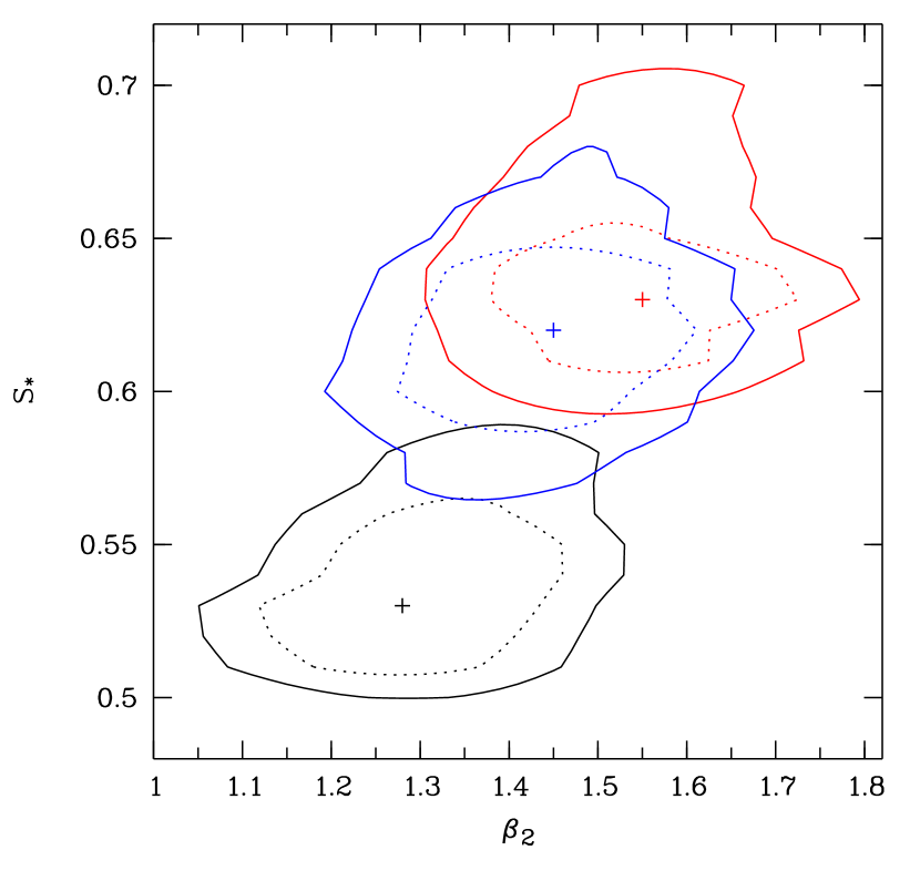
Figure 3: Maximum likelihood fit parameters $\beta_{2}$ and $S_{\ast}$ (in units of $10^{-14}$ $erg$ $cm^{-2}$ $s^{-1}$) to the 0.5-2 keV Log(N)-Log(S) for a broken power-law model (see text). Confidence contours are at 68% (dashed line) and at 90% (solid line) for two interesting parameters. The black contours are computed using a source characterization radius corresponding to an EEF of $\alpha=0.68$ and a source detection probability level of $p=2\times 10^{-4}$ for the Log(N)-Log(S). The red contours refer to $\alpha=0.80$ and $p=2\times 10^{-4}$ while the blue contours are computed with $\alpha=0.68$ and $p=2\times 10^{-5}$.

where $\beta_{1}$ is the power-law index at brighter fluxes, $\beta_{2}$ the index at fainter fluxes, $S_{\ast}$ is the flux of the break, $k_{1}$ and $k_{2}$ are the normalization factors ($k_{2}=k_{1}S_{\ast}^{\beta_{2}-\beta_{1}}$ to have continuity in the differential counts). Applying the maximum likelihood fit to the data, we obtain a best-fit value of $\beta_{1}=2.21^{+0.06}_{-0.09}$ (with a corresponding normalization $k_{1}=118.8^{+13.9}_{-11.1}$), while the confidence contours for $\beta_{2}$ and $S_{\ast}$, for each of the three Log(N)-Log(S) curves described earlier in this Section, are plotted in Figure 3. The break flux $S_{\ast}$, at 1$\sigma$ confidence level for two interesting parameters, ranges in a narrow interval of values, between $5\times 10^{-15}$ and $6.5\times 10^{-15}$ erg cm^-2 s^-1. The differential slope at fainter fluxes $\beta_{2}$ is not tightly constrained, ranging between 1.1 and 1.7 (1$\sigma$ confidence level for two interesting parameters). In any case, these values of $\beta_{2}$ are somewhat lower than those found by Hasinger et al. (1998) fitting the ROSAT data. The above authors find also a break at brighter fluxes: the discrepancy could arise from the fact that we are observing a fainter and flatter part of the Log(N)-Log(S), which was not accessible with the ROSAT PSPC data.
In the 2-10 keV energy band, we certainly have the largest hard X-ray selected sample available to date at these fluxes. Also in this case the data are in good agreement with previous determinations, by BeppoSAX (Giommi et al., 2000) and ASCA (Cagnoni et al., 1998; Ueda et al., 1999), in the brighter part, and by Chandra (Giacconi et al., 2001) in the fainter part. In this band, our Log(N)-Log(S) nicely fills in the gap between the Chandra deep surveys and the shallow BeppoSAX and ASCA surveys. A slight slope flattening (around $2\times 10^{-14}$ erg cm^-2 s^-1) comes out also in the 2-10 keV Log(N)-Log(S). A similar flattening has already been observed by Hasinger et al. (2001) in the Lockman Hole XMM-Newton deep observations. A maximum likelihood fitting technique has been applied also to the 2-10 keV Log(N)-Log(S). A single power-law model has its best-fit value at $\alpha=1.34^{+0.11}_{-0.10}$ and a normalization $K=229.2^{+29.3}_{-19.6}$. The K-S probability ($>10\%$) do not allow us to reject the model indicating that the flattening is not particularly significant. However the best-fit value of the slope is significantly sub-euclidean, in contrast to BeppoSAX and ASCA findings, indicating that probably the Log(N)-Log(S) flattens at faint fluxes.
The 5-10 keV Log(N)-Log(S) is in agreement, within the errors, with both XMM-Newton Lockman Hole data (Hasinger et al., 2001), which is a subsample of ours, and BeppoSAX HELLAS survey (Fiore et al., 2001b). Our Log(N)-Log(S) connects XMM-Newton deep observations with shallower BeppoSAX ones. The sample selected in this band (100 sources) is currently smaller than the BeppoSAX HELLAS sample (about 150 sources). However, we go deeper by an order of magnitude than the HELLAS survey and the error circle we can use in the optical follow up (conservatively we are assuming $3^{\prime\prime}$) is considerably smaller than BeppoSAX (about $1^{\prime}$), making the optical identification far easier.
A maximum likelihood fit of the 5-10 keV Log(N)-Log(S) with a single power-law model gives a value of $\alpha=1.54^{+0.25}_{-0.19}$ and a normalization $K=175.2^{+56.3}_{-36.2}$. As in the 2-10 keV band, the single power-law model is found to give an acceptable description of the data (the K-S probability is larger than $20\%$).
In each panel of Figure 2, the cyan dashed line represents the expected Log(N)-Log(S) from the improved Comastri et al. (1995) XRB synthesis model (see Comastri et al., 2001, for details). In the 0.5-2 keV band, the counts overestimates the model predictions at bright fluxes, because of the contribution from clusters and stars to the soft Log(N)-Log(S) . At fainter fluxes, where the AGN are the dominant contributors, the agreement is quite good. In the 2-10 keV band the agreement between XRB model predictions and our Log(N)-Log(S) is good at brighter fluxes, becoming marginal towards fainter fluxes. However, by varying the normalization of the model of $\sim 20\%$, the predicted Log(N)-Log(S) agrees well with both our data and CDFS data. In the 5-10 keV band the model predictions are in agreement within the errors with our Log(N)-Log(S) and the Lockman Hole and HELLAS surveys.
It is worth noting that we do not make any correction for confusion or Eddington biases. Nevertheless, the agreement between our source counts and Chandra and ROSAT data, in the 0.5-2 keV band, indicates that source confusion is still negligible at these fluxes.

6 Summary

We have carried out a serendipitous XMM-Newton survey. We cover nearly three square degrees in 15 fields observed during satellite calibration and performance verification phase. This is, to date, the XMM-Newton survey with the largest solid angle.
The present sample is one of the largest available in the 0.5-2 keV band and is surely the largest in the 2-10 keV band at these fluxes. In the 4.5-10 keV band we currently have a smaller sample than the BeppoSAX HELLAS survey. However, the flux limit is a factor about 10 deeper than HELLAS and the optical follow up of our survey is easier because of XMM-Newton better positional accuracy.
We computed the Log(N)-Log(S) curves in the 0.5-2 keV, 2-10 keV and 5-10 keV bands. Our measurements are in agreement with previous determinations by other satellites and XMM-Newton itself (Hasinger et al., 1998; Ueda et al., 1999; Cagnoni et al., 1998; Giommi et al., 2000; Giacconi et al., 2001; Hasinger et al., 2001) and with the predictions of the improved Comastri et al. (1995) XRB synthesis model.
In the hard bands, we sample an intermediate flux range: deeper than ASCA and BeppoSAX and shallower than Chandra and XMM-Newton deep pencil-beam surveys. It is worth to note that our approach is complementary to the latters: we probe large areas, at fluxes bright enough to allow, at least, a coarse spectral characterization of them. One of our main goals is in fact to find a good number of those rare objects (like type-2 QSOs) which are supposed to contribute significantly to the extragalactic hard X-ray background.
In the soft band, the Log(N)-Log(S) distribution shows a flattening around $5\times 10^{-15}$ erg cm^-2 s^-1. A similar result was also found from the ROSAT data (Hasinger et al., 1998). A broken power-law fit gives a differential slope index $\beta_{2}$ for the fainter part, flatter than Hasinger et al. (1998). The difference probably results from the fact that we are sampling different parts of the Log(N)-Log(S). A slight slope flattening of the Log(N)-Log(S) is also observed in the 2-10 keV band, around fluxes of $2\times 10^{-14}$ erg cm^-2 s^-1, although the data are consistent with a single power-law with a cumulative slope index $\alpha=1.34^{+0.11}_{-0.10}$. A single power-law fit is tenable also for the 5-10 keV Log(N)-Log(S) and gives a slope $\alpha=1.54^{+0.25}_{-0.19}$.
An extensive analysis of the X-ray broad-band properties of the sources and the optical follow-up of a hard X-ray selected sample will be the subjects of forthcoming papers (Baldi et al. in prep.).

Figure 1: The total sky coverage of the survey in the 0.5-2 keV (solid line), 2-10 keV (dashed line) and 4.5-10 keV band (dot-dashed line).

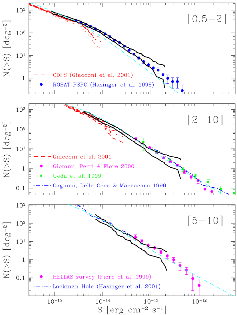
Figure 2: The cumulative Log(N)-Log(S) in the 0.5-2 keV (top), 2-10 keV (center) and 5-10 keV band (bottom). In all diagrams the black thick solid lines are the upper and lower limits of our Log(N)-Log(S), computed taking into account systematic effects, as described in Section 5. The cyan dashed line represents the predictions of the improved Comastri et al. (1995) XRB synthesis model (see details in text).

Table 1: The XMM-Newton Cal-PV field sample.

Revs	Target	$T_{MOS1}$(ks)	$T_{MOS2}$(ks)	$T_{pn}$(ks)	NH (cm-2)	$bII$(o)
51	PKS0537-286	19.0	37.0	36.6	$2.1\cdot 10^{20}$	-27.3
57	PKS0312-770	25.5	25.5	22.1	$8.0\cdot 10^{20}$	-37.6
63	MS0737.9+7441	37.3	38.5	31.6	$3.5\cdot 10^{20}$	29.6
70-71-73-74-81	Lockman Hole	84.6	86.2	104.9	$5.6\cdot 10^{19}$	53.1
75	Mkn 205	29.0	30.6	17.3	$3.0\cdot 10^{20}$	41.7
81-88-185	BPM 16274	38.9	39.2	33.0	$3.2\cdot 10^{20}$	-65.0
82	MS1229.2+6430	24.6		24.9	$2.0\cdot 10^{20}$	52.8
84-153	PKS0558-504	20.2	20.4	8.4	$4.5\cdot 10^{20}$	-28.6
84-165-171	Mkn 421	98.4	116.5		$7.0\cdot 10^{19}$	65.0
88	Abell 2690	17.5	17.5	16.2	$1.9\cdot 10^{20}$	-78.4
90	G158-100	21.3	16.6		$2.5\cdot 10^{20}$	-74.5
90	GD153	36.5	21.2	26.2	$2.4\cdot 10^{20}$	84.7
97	IRAS13349+2438	41.4			$1.2\cdot 10^{20}$	79.3
101	Abell 1835	27.7	27.7	22.9	$2.3\cdot 10^{20}$	60.6
161	Mkn 509	16.8	16.4		$4.1\cdot 10^{20}$	-29.9

References

- Akiyama et al. (2000) Akiyama, M. et al. 2000, ApJ, 532, 700
- Barger et al. (2001) Barger, A. J., Cowie, L. L., Mushotzky, R. F., & Richards, E. A. 2001, AJ, 121, 662
- Bower et al. (1996) Bower, R. G. et al. 1996, MNRAS, 281, 59
- Cagnoni et al. (1998) Cagnoni, I., Della Ceca, R., & Maccacaro, T. 1998, ApJ, 493, 54
- Comastri et al. (1995) Comastri, A., Setti, G., Zamorani, G., & Hasinger, G. 1995, A&A, 296, 1
- Comastri et al. (2001) Comastri, A., Fiore, F., Vignali, C., Matt, G., Perola, G. C., & La Franca, F. 2001, MNRAS, in press, astro-ph/0105525
- Crawford et al. (1970) Crawford, D. F., Jauncey, D. L., & Murdoch, H. S. 1970, ApJ, 162, 405
- Della Ceca et al. (2000) Della Ceca, R., Maccacaro, T., Rosati, P., & Braito, V. 2000, A&A, 355, 121
- Fabian & Iwasawa (1999) Fabian, A. C., & Iwasawa, K. 1999, MNRAS, 303, L34
- Fabian et al. (2000) Fabian, A. C. et al. 2000, MNRAS, 315, L8
- Fiore et al. (1999) Fiore, F., La Franca, F., Giommi, P., Elvis M., Matt, G., Comastri, A., Molendi, S., & Gioia, I. 1999, MNRAS, 306, L55
- Fiore et al. (2001a) Fiore, F., Comastri, A., La Franca, F., Vignali, C., Matt, G., & Perola, G. C. 2001a, in proceedings of the ESO/ECF/STSCI workshop on ”Deep Fields”, Garching October 2000, astro-ph/0102041
- Fiore et al. (2001b) Fiore, F. et al. 2001b, MNRAS, in press, astro-ph/0105524
- Franceschini et al. (2000) Franceschini, A., Bassani, L., Cappi, M., Granato, G. L., Malaguti, G., Palazzi, E., & Persic, M. 2000, A&A, 353, 910
- Gehrels (1986) Gehrels, N. 1986, ApJ, 303, 336
- Giacconi et al. (2001) Giacconi, R. et al. 2001, ApJ, 551, 624
- Gilli et al. (2001) Gilli, R., Salvati, M., & Hasinger, G. 2001, A&A, 366, 407
- Giommi et al. (2000) Giommi, P., Perri, M., & Fiore, F. 2000, A&A, 362, 799
- Hasinger et al. (1998) Hasinger, G., Burg, R., Giacconi, R., Schmidt, M., Trümper, J., & Zamorani, G. 1998, A&A, 329, 482
- Hasinger et al. (2001) Hasinger, G. et al. 2001, A&A, 365, L45
- Hornschemeier et al. (2001) Hornschemeier, A. E. et al. 2001, ApJ, 554, 742
- La Franca et al. (2001) La Franca, F., Fiore, F., Vignali, C., Comastri, A., & Pompilio, F. plus HELLAS consortium 2001, in proceedings of the Conference ”the New Era of Wide-Field Astronomy”, Preston (UK), 21-24 August 2000, astro-ph/0011008
- Miyaji et al. (2000) Miyaji, T., Hasinger, G., & Schmidt, M. 2000, A&A, 353, 25
- Murdoch et al. (1973) Murdoch, H. S., Crawford, D. F., & Jauncey, D. L. 1973, ApJ, 183, 1
- Mushotzky et al. (2000) Mushotzky, R. F., Cowie, L. L., Barger, A. J., & Arnaud, K. A. 2000, Nature, 404, 459
- Norman et al. (2001) Norman, C. et al. 2001, ApJ, submitted, astro-ph/0103198
- Ohta et al. (1996) Ohta, K., Yamada, T., Nakanishi, K., Ogasaka, Y., Kii, T., & Hayashida, K. 1996, ApJ, 458, L57
- Schmidt et al. (1998) Schmidt, M. et al. 1998, A&A, 329, 495
- Setti & Woltjer (1989) Setti, G., & Woltjer, L. 1989, A&A, 224, L21
- Stark et al. (1992) Stark, A. A., Gammie, C. F., Wilson, R. W., Bally, J., Linke, R. A., Heiles, C., & Hurwitz, M. 1992, ApJS, 79, 77
- Tozzi et al. (2001) Tozzi, P. et al. 2001, ApJ, in press, astro-ph/0103014
- Ueda et al. (1999) Ueda, Y. et al. 1999, ApJ, 518, 656
- Vignati et al. (1999) Vignati, P. et al. 1999, A&A, 349, L57
- Zamorani et al. (1999) Zamorani, G. et al. 1999, A&A, 346, 731