Period distribution of old accreting isolated neutron stars

In this paper we present calculations of period distribution for old accreting isolated neutron stars (INSs). After few billion years of evolution low velocity INSs come to the stage of accretion. At this stage INS’s period evolution is governed by magnetic braking and angular momentum accreted. Since the interstellar medium is turbulized accreted momentum can either accelerate or decelerate spin of an INS, therefore the evolution of period has chaotic character. Our calculations show that in the case of constant magnetic field accreting INSs have relatively long spin periods (some hours and more, depending on INS’s spatial velocity, its magnetic field and density of the surrounding medium). Such periods are much longer than the values measured by ROSAT for 3 radio-silent isolated neutron stars. Due to long periods INSs should have high spin up/down rates, $\dot{p}$, which should fluctuate on a time scale of $\sim 1$ yr.

1 Introduction

Spin period is one of the most precisely determined parameters of a neutron star (NS). Estimates of masses (for isolated objects), radii, temperatures, magnetic fields etc. are usually model dependent. That is why it is very important to have a good picture of evolution of the only model independent physical parameters of INSs — spin period and its derivative, as they are usually used to determine other characteristics of NSs. Our aim is to obtain distribution of periods $p$ for old accreting INSs (AINSs), we also briefly discuss possible values of period derivative $\dot{p}$.

A lot has been done to understand period evolution of radio pulsars (see Beskin et al. (1993)) and NSs in close binaries (Ghosh & Lamb (1979), Lipunov (1992)). AINS are especially interesting from the point of view of period (and by the way magnetic field) evolution since their history is not “polluted” by huge accretion, as it happens with their relatives in close binary systems, where NSs can accrete up to $1\,M_{\odot}$ during extensive mass transfer.

In early 90^s there has been a great enthusiasm about the possibility to observe a huge population of AINSs with ROSAT (Treves & Colpi (1991), Blaes & Rajagopal (1991), Blaes & Madau (1993), Madau & Blaes (1994)). However, it has become clear that AINSs are very elusive (Treves et al. (1998)) due to high spatial velocities (Popov et al. 2000a ) or/and magnetic field properties (Colpi et al. (1998), Livio et al. (1998)).

Still, AINSs (and radio-silent INSs in general) are a subject of interest in astrophysics (see Caraveo et al. (1996), Treves et al. (2000) and references therein). A few candidates seem to be observed by ROSAT (Motch (2001)), although it is also possible that these sources (at least a part of them) can be better explained by young cooling NSs (see Neühauser & Trümper (1999), Yakovlev et al. (1999), Walter (2001), Popov et al. 2000b ). Nevertheless, such sources should be very abundant at low fluxes available for Chandra and XMM–Newton observatories (in Popov et al. 2000b the authors obtain that at $\sim 10^{-13}$ erg s^-1 AINSs become more abundant than young cooling NSs, and expected number is about 1 source per square degree for fluxes $>10^{-16}$ erg s^-1), so the calculation of properties of AINSs is of great importance now.

Previous estimates of spin properties of AINSs (Lipunov & Popov 1995a , Konenkov & Popov (1997)) have given only typical values of periods, no realistic distributions of this parameter are calculated. “Spin equilibrium” of NSs with the interstellar medium (ISM) has been always assumed, i.e. the authors have considered the situation, when all INS have enough time for spin evolution, they have not considered NSs with relatively high spatial velocities. In this paper we present full analysis of the problem.

Period estimates are especially important as far as this parameter can be used to distingush accreting INSs from young cooling NSs and background objects.

We proceed as follows: In the next section we describe the model used to calculate period distribution. In Section 3 we present our results. In this paper we do not address the question of the total number of AINS, for this data we refer to our previous calculations (Popov et al. 2000a , Popov et al. 2000b ). Here we only show period distributions for AINSs. In the last section we give a brief discussion, derive typical parameters of $\dot{p}$ for AINSs and summarize the paper.

2 Model

In this section we describe our model of spin evolution of AINS in turbulent ISM. We consider constant ISM density and isotropic Kolmogorov turbulence (Kolmogorov spectrum is in good correspondence with most of observation of interstellar, i.e. intercloud, turbulence, see for example Falgarone & Philips (1990)). Orientations of turbulent cells at all scales are assumed to be independent. Turbulent velocities at different scales relate to each other according to the Kolmogorov law:

$$\frac{v_{t}(r_{1})}{v_{t}(r_{2})}=\left(\frac{r_{1}}{r_{2}}\right)^{1/3}\,.$$

Observations show (see Ruzmaikin et al. (1988) and references therein) that turbulent velocity at the scale of $R_{t}\simeq 2\cdot 10^{20}\textrm{\leavevmode\nobreak\ cm}\simeq 70$ pc is about $v_{t}\simeq 10$ km s^-1. The scale above is close to the thickness of the gas disk of the Galaxy, and the velocity above — to the speed of sound in the ISM. It corresponds to the largest cell size possible and the fastest movements (otherwise turbulence will efficiently dissipate its energy in shocks).

As an AINS moves through the ISM it can capture matter inside so called Bondi (or accretion, or gravitational capture) radius, $R_{G}=2GM/v^{2}$. Here $G$ is the gravitational constant, $M$ is the mass of NS, $v=\sqrt{v^{2}_{NS}+v^{2}_{s}\,}$, $v_{NS}$ is the spatial velocity of a NS relative to ISM, $v_{s}$ is the speed of sound (we assume $v_{s}=10$ km s^-1, $M=1.4\,M_{\odot}$ everywhere in the paper; $v_{s}$ can be dependent on the luminosity of AINS (Blaes et al. (1995)), but here we neglect it planning to iclude this dependence in our future calculations).

Accretion rate $\dot{M}$ at the conditions stated above is equal to (Hoyle & Littleton (1939), Bondi & Hoyle (1944)):

$$\dot{M}=\pi R_{G}^{2}nm_{p}v\,,$$

here $n$ is the number density of the ISM, $m_{p}$ is the mass of proton. This accretion rate corresponds to luminosity:

$$L=GM\dot{M}/R\sim 10^{32}n\,(v/10\,{\rm km}\,{\rm s}^{-1})^{-3}\,{\rm erg}\,{\rm s}^{-1}$$

Based on population synthesis models (Popov et al. 2000b ) we can expect, that on average AINS should have luminosities about $10^{29}$ erg s^-1. Simple calculations show, that most of this energy will be emitted in X-rays with a typical blackbody temperature about 0.1 keV (if due to significant magnetic field accretion proceeds onto small polar caps then the temperature would be higher up to 1 keV). Note, that Bondi rate is just the upper limit, in reality due to heating (Shvartsman 1970a , Shvartsman (1971), Blaes et al. (1995)) and magnetospheric effects (Toropina et al. (2001)) the accretion rate can be lower.

Due to the turbulence accreted matter carries non-zero angular momentum:

$$j_{t}=v_{t}(R_{G})\cdot R_{G}=v_{t}(R_{t})R_{t}^{-1/3}R_{G}^{4/3}\,.$$

In this formula it is considered that cells of the size $r=R_{G}$ are the most important, otherwise in the Eq.(1) below it is necessary to introduce factor $\alpha\neq 1$.

If $j_{t}$ is larger than the Keplerian value on the magnetosphere boundary (i.e. on the Alfven radius $R_{A}=(\mu^{2}/2\dot{M}\sqrt{GM\,})^{2/7}$, here $\mu$ is the magnetic moment of a NS) an accretion disk is formed around the AINS. In the disk a part of the angular momentum is carried outwards, and the NS accrets matter with Keplerian angular momentum $j_{K}=v_{K}(R_{A})\cdot R_{A}$, $v_{K}$ – Keplerian velocity. This situation holds only for very low magnetic fields and low spatial velocities of NSs, thus we do not take it into account in the present calculations.

We consider the lowest spatial velocity of NSs to be equal to 10 km s^-1. This value is of order of the speed of sound. Therefore lower spatial velocities can not change the accretion rate significantly. Moreover such low values are not very probable due to non-zero spatial velocities of NSs progenitors (see Popov et al. 2000a , Arzoumanian et al. (2001) for limits onto the fraction of low velocity INSs derived by different methods). For several cases below we consider $v\simeq v_{NS}$.

During the time required to cross a turbulent cell of the size $R_{G}$, $\Delta t=R_{G}/v_{NS}\simeq 11.8\,(v/10\,\textrm{km\leavevmode\nobreak\ s}^{-1})^{-3}$ yrs, the change in the angular momentum of a NS $J$ is given as:

$$\left|\@vec{\Delta J}\right|=\dot{M}j_{t}\Delta t=\pi nm_{p}v_{t}(R_{t})R_{t}^{-1/3}R_{G}^{13/3}$$

$$\simeq 1.23\cdot 10^{39}\,{\rm g\,cm^{2}\,s}^{-1}\times$$

$$\,n\left(\frac{v_{t}(R_{t})}{10\,{\rm km\,s}^{-1}}\right)\left(\frac{R_{t}}{2\cdot 10^{20}\,{\rm cm}}\right)^{-1/3}\left(\frac{v}{10\,{\rm km\,s}^{-1}}\right)^{-26/3}\,.$$

Accordingly, the change of the spin frequency reads:

$$\left|\@vec{\Delta\omega}\right|=\left|\@vec{\Delta J}\right|/I$$

$$\simeq 1.23\cdot 10^{-6}\,{\rm s}^{-1}\times$$

$$\,n\left(\frac{v_{t}(R_{t})}{10\,{\rm km\,s}^{-1}}\right)\left(\frac{R_{t}}{2\cdot 10^{20}\,{\rm cm}}\right)^{-1/3}\left(\frac{v}{10\,{\rm km\,s}^{-1}}\right)^{-26/3}I_{45}^{-1}\,,$$

here $I=I_{45}10^{45}$ g cm² — moment of inertia of a NS. Orientation of $\@vec{\Delta\omega}$ is random, and it is isotropically distributed on the sphere. The value of the frequency change is strongly dependent on the spatial velocity of the NS: $\Delta\omega\sim v^{-26/3}$, so the maximum value for $v_{NS}=10$ km s^-1 is $\Delta\omega_{\max}\simeq 6\cdot 10^{-8}$ rad s^-1.

On this view, it follows that it is possible to describe the spin evolution of an AINS as random movement in 3-D space of angular velocities $\@vec{\omega}$. Since typical temporal and “spatial” scales $\Delta t$ and $\Delta\omega$ are reasonably small ($\Delta t\ll t_{gal}\simeq 10^{10}$ yrs, $\Delta\omega\ll\omega\sim 10^{-1}\div 10^{-7}$ rad s^-1) we consider the problem to be continuous. Therefore, we can use differential equations valid for continuous processes.

In this case the spin evolution of an AINS in the space $\@vec{\omega}$ is described by the diffusion equation with the coefficient, namely:

$$D=\frac{\alpha}{6}\frac{\Delta\omega^{2}}{\Delta t},$$ (1)

here $\alpha$ — coefficient which takes into account cells with sizes $r\neq R_{G}$ (everywhere in this paper we use $\alpha=1$).

Besides random turbulent influence an AINS is spinning down due to magnetic braking:

$$\frac{d\@vec{\omega}}{dt}=\kappa_{t}\frac{\mu^{2}}{IR_{co}^{3}}\frac{\@vec{\omega}}{|\omega|}+\@vec{F}_{t}=\kappa_{t}\frac{\mu^{2}}{IGM}\omega^{2}\frac{\@vec{\omega}}{|\omega|}+\@vec{F}_{t}\,.$$ (2)

Here $R_{co}=(GM/\omega^{2})^{1/3}$ — corotation radius, $\kappa_{t}$ — constant of the order of unity, which takes into account details of interaction between the magnetosphere and accreted matter (everywhere in this paper we accept $\kappa_{t}=1$), $\@vec{F}_{t}$ — random (turbulent) force with zero average value: $\langle\@vec{F}_{t}\rangle=0$.

On large time scale and for relatively short spin periods we can neglect momentum of the accreted matter and initial period of NS $p_{0}$. In that case solution of Eq. (2) looks as:

$$\omega\propto t^{-1}\,,\quad p\equiv\frac{2\pi}{\omega}\propto t\,.$$

Magnetic braking produces a convective term in the evolutionary equation for spin frequency distribution, $f(\omega)$. As far as initial distribution of spin vectors is isotropic (magnetic braking does not change the orientation of $\@vec{\omega}$) and turbulent diffusion is isotropic too, we obtain spherically symmetric distribution in the space of angular velocities, i.e.:

$$f(\@vec{\omega})=f_{3}(\omega)$$

($f_{3}(\omega)$ describes 3-D distribution of AINSs, its dimension is $[\textrm{s}^{-3}]$).

From (1) and (2) we obtain the evolutionary equation:

$$\frac{\partial f_{3}}{\partial t}=\frac{A}{\omega^{2}}\frac{\partial}{\partial\omega}\left(\omega^{4}f_{3}\right)+\frac{D}{\omega^{2}}\frac{\partial}{\partial\omega}\left(\omega^{3}\frac{\partial f_{3}}{\partial\omega}\right)\,,$$ (3)

here $A=\left(\mu^{2}/IGM\right)$.

Boundary condition at $\omega=0$ can be derived from the equality of the flow of the particles at this point to zero:

$$\left.\frac{\partial f_{3}}{\partial\omega}\right|_{\omega=0}=0\,.$$

It is easy to find stationary solution of the equation (3) on the semi-infinity axis ($\omega\geq 0$)

$$f_{3}^{\textrm{\scriptsize\,st}}=C_{st}\exp\left(-\,\frac{\mu^{2}}{3\,IGMD}|\omega|^{3}\right)\,,$$ (4)

here normalization constant $C_{st}$ can be derived from the condition $4\pi\int f_{3}^{\textrm{\scriptsize\,st}}(\omega)\omega^{2}d\omega=N$, $N$ — full number of AINSs in the distribution. Total number of NSs in the Galaxy is uncertain, $N\sim 10^{8}$–$10^{9}$. Population synthesis calculations (Popov et al. 2000b ) give arguments for higher total number about $10^{9}$. Here we do not address this question. From the curves below, which represent relative period distribution of AINSs, one can determine absolute numbers of AINSs with each period value if the total number of these objects is known.

Position of the maximum of $f_{3}^{\textrm{\scriptsize\,st}}(p)$ depends on $v$, $\mu$, $n$ and $M$. Increasing of $v$ and $\mu$ shifts the maximum to larger $p$, increasing of $n$ and $M$ — to shorter $p$.

If we have to solve the problem for constant starformation rate we can write second boundary condition as:

$$f_{3}(\omega_{\mathrm{\scriptsize A}})=\frac{IGM}{4\pi\kappa_{t}\mu^{2}}\cdot\frac{\dot{N}}{\omega_{\mathrm{\scriptsize A}}^{4}}\,,$$

here $\dot{N}$ — rate at which NSs come to the stage of accretion, $\omega_{\mathrm{\scriptsize A}}=2\pi/p_{A}$ — accretor frequency, at that value for given $v$ and $n$ accretion sets on, $p_{A}=2^{5/14}\pi(GM)^{-5/7}(\mu^{2}/\dot{M})^{3/7}\simeq 300\,\mu_{30}^{6/7}(v/10\,{\rm km}\,{\rm s}^{-1})^{9/7}n^{-3/7}\,{\rm s}$.

The function $f_{3}(\omega)$ is connected with distributions of absolute values of the angular velocity, $f_{1}(\omega)$, and of the spin period, $f(p)$, according to the formulae:

$$f_{1}(\omega)=4\pi\omega^{2}f_{3}(\omega)\,,$$

$$f(p)=\frac{32\pi}{p^{4}}f_{3}\left(\frac{2\pi}{p}\right)\,.$$

Figure 1 shows the evolution of $f(p)$ as a function of time for typical parameters of an AINS and the ISM.

Figure 1: Evolution of the period distribution in time; $\mu=10^{30}$ G cm³, $n=1$ cm^-3, $v_{NS}=10$ km s^-1. Curves are plotted for 4 different moments from $1.72\cdot 10^{9}$ yrs to $9.8\cdot 10^{9}$ yrs ($t_{A}$ for chosen parameters is equal to $\simeq 1.7\cdot 10^{9}$ yrs). An AINS crosses the horizontal part from $\simeq 10^{2}$ s to $10^{4}$ s in $\sim 6\cdot 10^{7}$ yrs. Curves were normalized to 1 in the maximux for the highest curve.

For given $v$, $\mu$ and $n$ NSs enter the accretor stage when they spin down to $p_{\mathrm{\scriptsize A}}$. Up to this value they evolve as ejectors and propellers (Lipunov (1992), Colpi et al. (2001)).

For $p_{\mathrm{\scriptsize A}}<p<p_{cr}$ influence of the turbulence is small and AINS spin down according to $p\propto t$. Here $p_{cr}$ defines the stage when spin changes due to magnetic braking and turbulent acceleration/decelaration become of the same order of magnitude (see below the Discussion). One can introduce another useful timescal, $\Delta t_{cr}$. This is the time required to reach turbulent regime, $p=p_{cr}$. These considerations together with constant starformation rate determine left part of the distribution where $f(p)=const$ (see Fig. 1).

As the period grows turbulence becomes more and more important. Finally the first AINSs reach the point $p=\infty$ ($\omega=0$) and there equilibrium component of the distribution (described by Eq. (4) is formed quickly. This component decreases in a power law fashion ($f(p)\propto p^{-4}$) at $p\gg p_{turb}$ (where $p_{turb}$ is determined by the width of the distribution (4)), and decreases even faster than exponentially at $p\ll p_{turb}$. Please note that the number of AINSs reaching equilibrium grows linearly with time. As a result, the amplitude of equilibrium component of the distribution grows likewise. If the time required to reach the accretor stage, $t_{A}$, is large ($t_{gal}-t_{\mathrm{\scriptsize A}}\ll t_{gal}$) the equilibrium component is not formed. For $t_{\mathrm{\scriptsize A}}>t_{gal}$ NS never reach the stage of accretion.

Similar considerations can be applied also to binary X-ray pulsar (see Lipunov (1992)). In binaries NSs can reach real period equilibrium (Ghosh & Lamb (1979)), and stationary solution should be used. In that case observations of period fluctuations can help to derive physical parameters of the systems, for example stellar wind velocity for wind-fed pulsars (Lipunov & Popov 1995b ).

3 Calculations and results

The main aim of this paper is to obtain period distribution for AINS in turbulized ISM. We assume that NS are born with short ($\ll 1$ s) spin periods. Magnetic moment distribution is taken in log-Gaussian form:

$$f(\mu)=\frac{1}{\sqrt{2\pi\sigma_{m}\,}}\exp\left(\frac{(\log\mu-\log\mu_{0})^{2}}{2\sigma_{m}^{2}}\right)\,,$$ (5)

with $\log\mu_{0}=30.06$ and $\sigma_{m}=0.32$ (see Colpi et al. (2001) and references therein for a recent discussion and data on magnetism in NSs). Magnetic field is considered to be constant (see, for example, Urpin et al. (1996) for calculations of magnetic field decay and related discussion).

Velocity distribution (due to kick after supernova explosion) is assumed to be Maxwellian:

$$f(v_{NS})=\frac{6}{\sqrt{\pi}}\frac{v_{NS}^{2}}{v_{m}^{2}}\exp\left(\frac{3}{2}\frac{v_{NS}^{2}}{v_{m}^{2}}\right)$$ (6)

with $v_{m}=200$ km s^-1 which corresponds to $\sigma_{v}\simeq 140$ km s^-1 (see for example Lyne & Lorimer (1994), Cordes & Chernoff (1997), Hansen & Phinney (1997), Lorimer et al. (1997), Cordes & Chernoff (1998), and Arzoumanian et al. (2001) for discussions on the kick velocity of NSs).

We use two values of the ISM number density, $n=1$ cm^-3 and $n=0.1$ cm^-3, as typical values for the Galactic disk .

All NS are divided into 30 groups in $\mu$ interval from $10^{28.6}$ to $10^{31.6}$ G$\cdot$cm³ with the step 0.1 dec and 49 groups in velocities from 10 to 500 km s^-1 with the step 10 km s^-1.

For each group we calculate $t_{A}$, the time necessary to reach accretion:

$$t_{A}=t_{E}+t_{P}\,,$$

here $t_{E}$ and $t_{P}$ — durations of the ejector and propeller stages correspondently.

On the stage of ejection a NS spin down due to magneto-dipole losses:

$$t_{E}\simeq 10^{9}n^{-1/2}\left(\frac{v}{10\leavevmode\nobreak\ \textrm{km}\,\textrm{s}^{-1}}\right)\left(\frac{\mu}{10^{30}\leavevmode\nobreak\ \textrm{G}\cdot\textrm{cm}^{3}}\right)^{-1}\leavevmode\nobreak\ \mbox{yrs.}$$

Spin down on the propeller stage (Shvartsman 1970b , Illarionov & Sunyaev (1975)) is not well known, but for constant field always $t_{P}<t_{E}$ (Lipunov & Popov 1995a ) (see also results of numerical calculations in Toropin et al. (1999)), so we neglect $t_{P}$ in the rest of the paper, i.e. we assume $t_{A}=t_{E}$.

For high spatial velocities after ejector an INS appears not as a propeller, but as a so-called georotator (Lipunov (1992), see also Rutledge (2001)). At this stage $R_{A}>R_{G}$, so surrounding matter does not feel gravitation of the NS, and its magnetosphere looks like magnetospheres of the Earth, Jupiter etc. Partly because of that effect we truncated our velocity distribution at 500 km s^-1.

For systems with $t_{A}<t_{gal}=10^{10}$ yrs we solve Eq. (3) on the time interval $t_{gal}-t_{A}$. For angular velocities we use grid with 200 cells from $\omega=0$ to $\omega_{A}$. Conservative implicit scheme is used. Derived distributions $f(p,\mu,v)$ (for different groups) are summed with weights from Eqs. (5) and (6).

Figure 2: Period distribution for populations of AINSs evolving in the ISM with number density $n=1$ cm^-3 (upper solid curve) and $n=0.1$ cm^-3 (the second dotted curve). Lower curves show results for low velocity part of AINS population for $n=0.1$ cm^-3 ($v<60,\,30,\,15$ km s^-1 correspondently, see Discussion below). Curves for normalized to 1 in maximum for the highest curve.

Final distribution for $n=1$ cm^-3 and $n=0.1$ cm^-3 are shown on Fig. 2.

We note, that the final distribution significantly differs from the one for a single set of parameters ($n,\mu,v$): compare Fig. 1 and Fig. 2. In the final one we see power-law cutoff ($f\propto p^{-4}$) at long periods ($p>10^{7}$ s) similar to cutoff on the Fig. 1. Then at the intermediate periods ($10^{4}<p<10^{7}$ s) the curve has power-law ascent due to summation of individual curves maxima. Finally a sharp cutoff at short periods ($p<10^{4}$ s) is presented because different INSs enter the accretor stage with different periods: $p_{A}=p_{A}(n,\mu,v)$.

4 Discussion and conclusions

After an INS comes to the stage of accretion ($p>p_{A}$) its spin is controlled by two processes (see Eq.2): magnetic spin-down and turbulent spin-up/spin-down. Schematic view of such evolution process is shown on Fig. 3.

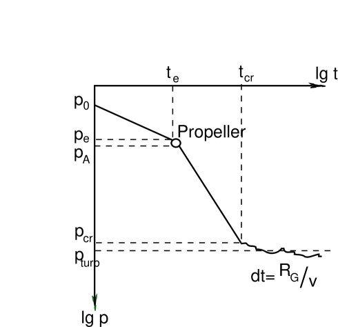
Figure 3: Schematic view of period evolution of an INS. A NS starts with $p=p_{0}$, then spins down according to magneto-dipole formula up to $p_{E}$, then a short propeller stage (marked by a circle) appears and lasts down to $p=p_{A}$. At the situation illustrated in the figure $t_{E}\approx t_{A}$. On the stage of accretion at first magnetic braking is more important, after at $t=t_{cr}$ turbulence starts to influence significantly spin evolution of a NS period stars to fluctuate with a typical time scale $R_{G}/v_{NS}$ close to mean value noted $p_{turb}$ on the vertical axis.

We can describe them with characteristic timescales: $t_{mag}$ and $t_{turb}$. As one can calculate, $t_{mag}\sim p$ and $t_{turb}\sim p^{-1}$. Here we evaluate $t$ as $p/\dot{p}$, and $\dot{p}_{turb}=p^{2}\dot{M}j/(2\pi I)$. Here we again note, that $j_{t}$ can be larger that the Keplerian value of angular momentum on the magnetosphere, $j_{K}=v_{K}(R_{A}),R_{A}$. So we write $j$ instead of $j_{t}$ as we did before, now $j={\min}(j_{K},j_{t})$.

$$\dot{p}_{mag}=2\pi\mu^{2}/(IGM)$$ (7)

Initially (immediately after $p=p_{A}$) magnetic spin-down is more significant:

$$t_{mag}=\frac{IGM}{2\pi\mu^{2}}p,$$ (8)

but at some period, $p_{cr}$, these two timescales should become of the same order, and for longer periods an INS will be governed mainly by turbulent forces.

One can obtain the following formula:

$$p_{cr}^{2}=\frac{4\pi^{2}\mu^{2}}{GM\dot{M}j}.$$ (9)

This period lies between $p_{A}$ and $p_{turb}$. An INS reach $p_{cr}$ in $\Delta t_{cr}\sim 10^{5}$–$10^{7}$ yrs after onset of accretion:

$$\Delta t_{cr}=\frac{I\sqrt{GM}}{\mu\sqrt{\dot{M}j}}.$$ (10)

Here $\Delta t_{cr}$ are calculated approximately as $p_{cr}/\dot{p}_{mag}$.

The period evolution of an AINS can be described in the following way (Fig. 3): after the INS comes to the stage of accretion it spins down for $\sim 10^{5}-10^{7}$ yrs up to $p_{cr}$, then the evolution is mainly controlled by the turbulence, and period fluctuates with typical value $p_{turb}$, which is determined by the properties of the surrounding ISM and spatial velocity of an INS.

We note, that we do not take into account any selection effects. For example, as far as period and luminosity both depend on the velocity of an INS, they are correlated. Taking into account flux limits of the present day satellites it is possible to calculate probability to observe an accreting INS with some period. Also periods (and luminosities) are correlated with position of an INS in the Galaxy.

So, it is reasonable to make calculations which include all that effects in order to make better predictions for observations. We plan to unite our population synthesis calculations with detailed calculations of spin evolution later. In this paper we present distributions as if all accreting INSs can be observed.

For the main part of its life spin period of a low-velocity AINS is governed by turbulent forces. Characteristic timescale for them can be written as: $t_{turb}=I\omega/(\dot{M}j)$. And it is equal to $10^{4}$-$10^{5}$ yrs for typical parameters.

For field decay picture should be completely different (see for example Konenkov & Popov (1997), Wang (1997)), and observations of AINSs can put important limits onto models of magnetic field decay in NS (Popov & Prokhorov (2000)). For decaying fields AINSs can appear as pulsating sources with periods about 10 s and $\dot{p}$ about $10^{-13}$ s/s (Popov & Konenkov (1998)). The value and sign of $\dot{p}$ will fluctuate as an INS passes through the turbulent cell on a time scale $R_{G}/v_{NS}$, which is about a year for typical parameters. Irregular fluctuations of $\dot{p}$ on that time scale can be significant indications for accretion (vs. cooling) nature of observed luminosity.

Roughly $\dot{p}$ can be estimated from the expression:

$$|\dot{p}|\leq p^{2}\frac{\dot{M}j}{2\pi I}\sim v^{-17/3}.$$ (11)

Here we neglect magnetic braking in Eq. (2). This equation for $\dot{p}$ is valid for turbulent regime of spin evolution, i.e. for $p\gg p_{turb}$. For the given $p$ value of $\dot{p}$ fluctuates between $+p^{2}\frac{\dot{M}j}{2\pi I}$ and $-\,p^{2}\frac{\dot{M}j}{2\pi I}$, and depends on $n$, $v$, but not on $\mu$ (if $j=j_{t}$, not $j=j_{A}$). In this picture $\dot{p}$ distribution in the interval specified above (Eq.11) is flat.

Behavior of $p$ and $\dot{p}$ of AINSs in molecular clouds can be different (Colpi et al. (1993)), especially for low spatial velocities of NSs. Some of our assumptions in that case are not valid, and results cannot be applied directly. But we note, that passages through molecular clouds are relatively rare and short, they cannot significantly influnce the general picture of AINSs spin evolution.

Period distribution which can be obtained from observation (for example from ROSAT data) can be different from two upper curves on the Fig. 2. Such surveys are flux-limited, so they include (in the case of AINS) the most luminous objects. But they form only a small fraction of the whole population.

To illustrate it on the Fig. 2 we also plot distributions for low velocity objects ($v<60,30,15$ km s^-1). In the case of fixed ISM density an upper limit on the value of the spatial velocity corresponds to a lower limit on the accreting luminosity of an AINS. Clearly, brighter the source — shorter (on average) its spin period. Even in that groups with relatively short periods their values are far from typical periods of ROSAT INSs, $\sim 5-20$ s. So, these objects cannot be explained by accretors with constant field $B\sim 10^{12}$ G.

Calculations of period distributions for decaying magnetic field, for populations of INSs with significant fraction of magnetars and for accretion rate different from the standart Bondi-Hiyle-Littleton value (due to heating and influence of a magnetosphere) will be done in a separate paper.

In conclusion we stress readers attention on the main results of the paper:

• we obtained spin period distributions for AINSs with constant magnetic field and “pulsar” properties (field, initial periods and velocity distributions).

• these distributions are shown in Fig. 2. They have broad maximum at very long periods, $\sim 10^{6}$ s. In that case observed objects should not show any periodicity.

• periods of these objects should fluctuate on a time scale $R_{G}/v_{NS}\sim 1$ yr.