Correlation of the magnetic field and the intra-cluster gas density in galaxy clusters

We present a correlation between X-ray surface brightness and Faraday rotation measure in galaxy clusters, both, from radio and X-ray observations as well as from modeling of the intra-cluster medium. The observed correlation rules out a magnetic field of constant strength throughout the cluster. Cosmological, magneto-hydrodynamic simulations of galaxy clusters are used to show that for a magnetic field of cosmic origin this correlation is expected and excellently reproduces the observations showing that the RMS scatter of the Faraday rotation increases linearly with the X-ray surface brightness. From the correlation between the observable quantities, rotation measure and X-ray surface brightness, we infer a relation between the physical quantities: magnetic field and gas density. For the best available observations, those of A119, we find $B\propto n_{e}^{0.9}$.

1 Introduction

It is now well established that the intra-cluster medium (ICM) in clusters of galaxies is magnetized. The presence of cluster magnetic fields is directly demonstrated by the existence of diffuse cluster-wide synchrotron radio emission (radio halos and relics) as revealed in the Coma cluster (Giovannini et al. 1991, 1993) and some other clusters (e.g., Feretti 1999). Under the assumption that the energy density within radio sources is minimum (equipartition condition), magnetic field values in the range 0.1-1 $\mu$G are derived for the radio emitting regions, i.e. on scales as large as $\sim 1$ Mpc. These values are consistent with those suggested from the recent detections of Inverse Compton hard X-ray emission in clusters with halos or relics (Bagchi et al. 1998, Fusco-Femiano et al. 1999, 2000, Rephaeli et al. 1999).

In addition, indirect observational evidence for the existence of cluster magnetic fields can be inferred from rotation measure (RM) studies of extragalactic radio sources located within or behind the clusters. Kim et al. (1991) analyzed the RM of radio sources in a sample of Abell clusters and found that $\mu$G level fields are widespread in the ICM, regardless of whether there is a strong radio halo or not. In a recent statistical study, Clarke et al. (2001) found that the ICM in clusters is permeated with a high filling factor by magnetic fields at levels of 4 - 8 $\mu$G and with a correlation length of $\sim$15 kpc, up to $\sim$0.75 Mpc from the cluster center. In Coma, A119 and in the 3C129 cluster, Feretti et al. (1995), Feretti et al. (1999) and Taylor et al. (2001) found a magnetic field component between 5 and 10 $\mu$G, tangled on scales of a few kpc. In Coma, the existence of a weaker magnetic field component, ordered on a scale of about one cluster core radius and with a strength of 0.1-0.2 $\mu$G was also inferred. Strong magnetic fields, up to the extreme value of tens of $\mu$G have been found in clusters with “cooling flows” (e.g., Hydra A, Taylor & Perley 1993; 3C295, Allen et al. 2001), where it has been suggested that the cooling flow process may play a role in magnetic field amplification (Soker & Sarazin 1990, Godon et al. 1998).

The magnetic field strengths obtained from RM arguments are therefore higher than the values derived either from the radio data, and or from Inverse-Compton X-ray emission. We note, however, that values deduced from radio synchrotron emission and from inverse Compton refer to averages over large volumes. Instead RM estimates give a weighted average of the field and gas density along the line of sight, and could be sensitive to the presence of filamentary structure in the cluster and/or to the existence of local turbulence around the radio galaxies. They could therefore be higher than the average cluster value (see also Goldshmidt & Rephaeli 1993). From the observational evidence, we can generally conclude that clusters of galaxies are pervaded by magnetic fields at least of the order of $\sim\mu$G. According to these findings, the energy associated with the magnetic field is comparable to the turbulent and thermal energy, i.e. the fields are strong enough to be dynamically important in a cluster.

The observations are often interpreted in terms of the simplest possible model, i.e. in this case a constant field throughout the whole cluster. However, Jaffe (1980) suggested that the magnetic field distribution depends on the thermal gas density and on the distribution of massive galaxies and therefore would decline with the cluster radius, as also derived by Brunetti et al. (2001) in Coma.

The knowledge of the properties of the large-scale magnetic fields in clusters is important for studying cluster-formation and evolution, and has significant implications for primordial star formation (Pudritz & Silk 1989). The magnetic fields could be primordial (Olinto 1997), or injected into the ICM from galactic winds or from active galaxies (Kronberg et al. 1999, Völk & Atoyan 1999). The seed fields, whose strengths have been calculated to be up to 10^-9 G (see Kronberg 1994, Blasi et al. 1999), are likely to be amplified by turbulence following a cluster merger (Tribble 1993, Dolag et al. 1999). Amplification by turbulence excited by galactic motions (Jaffe 1980, Ruzmaikin et al. 1989) has been shown to be insufficient to create magnetic fields of the appropriate strength (De Young 1992, Goldshmidt & Rephaeli 1993).

In this paper we use the cosmological magneto-hydrodynamic code (MHD) presented by Dolag et al. (1999) to derive the magnetic field of clusters of galaxies. We compare this magnetic field with the X-ray flux as a function of distance to the cluster center. We then perform the same comparison with quantities from observations, i.e. the X-ray surface brightness and the RM, for four clusters: Coma, A119, A514 and 3C129. The correlations found, both in simulations and in observations, allow conclusions to be drawn about the connection between magnetic field and the gas density in clusters.

The paper is organized as follows: Sect. 2 summarizes the simulations we have performed, Sect. 3 gives the relation between the X-ray surface brightness $S_{x}$ and the root mean square of the rotation measure $\sigma_{\mathrm{RM}}$ obtained from the simulations, Sect. 4 presents the available radio and X-ray data, which are compared with the simulations in Sect. 5. In Sect. 6 we draw conclusions about the correlation of the gas density and the magnetic field.

2 Simulations

We use the cosmological MHD code described in Dolag et al. (1999) to simulate the formation of magnetized galaxy clusters from an initial density perturbation field. The evolution of the magnetic field is followed starting from an initial seed field. This field is amplified by compression during cluster collapse. Merger events and shear flows, which are very common in the cosmological environment of large-scale structure, lead to Kelvin-Helmholtz instabilities. They further increase the field strength by a large factor. In order to reproduce the present $\mu$G fields, an initial field strength of $10^{-9}$G is required. In such a scenario the final magnetic field structure is produced by the formation of the galaxy cluster in the context of large-scale evolution. This means that the final magnetic field properties are predictions of our understanding of the formation of galaxy clusters, under the assumption that the magnetic field in galaxy clusters results from amplification of weak seed fields. Our models are able to reproduce the observed Faraday rotation measures very well.

2.1 GrapeMSPH

The code combines the merely gravitational interaction of a dark-matter component with the magneto-hydrodynamics of a gaseous component. Gravitational forces are calculated on the special-purpose hardware component Grape 3Af (Ito et al. 1993) which is connected to the host computer. Given a collection of particles, their masses and positions, the Grape board computes their mutual distances and the gravitational forces between them, smoothed at small distances according to the Plummer law. The gas dynamics is computed in the smoothed particle (SPH) approximation which benefits from the list of neighboring particles also returned by the the Grape board. It is supplemented with the magneto-hydrodynamic equations to trace the evolution of the magnetic fields which are frozen into the motion of the gas because of its assumed high electric conductivity. The backreaction of the magnetic field on the gas is included. Extensive tests of the code were successfully performed and described in a previous paper (Dolag et al. 1999). $\@vec{\nabla}\cdot\@vec{B}$ is always negligible compared to the magnetic field divided by a typical length scale of the magnetic field within the simulations, e.g. 50-100 kpc. The code also assumes the ICM to be an ideal gas with an adiabatic index of 5/3 and neglects radiative cooling. The surroundings of the clusters are dynamically important because of tidal influences and the details of the merger history. In order to account for this the cluster simulation volumes are surrounded by a layer of boundary particles in order to represent accurately the sources of the tidal fields in the cluster neighborhood. The details of the code, the models and the obtained magnetic field structure will be presented in a forthcoming paper (Dolag et al., in preparation).

2.2 Initial conditions

As shown in Dolag (2000) the magnetic fields in our simulations reproduce the Faraday rotation observations independent of the chosen cosmology. Therefore we restrict for these comparisons our models to one SCDM cosmology ($\Omega_{\mathrm{m}}^{0}=1.0$, $\Omega_{\Lambda}^{0}=0$, $H_{0}=50\,{\rm km\,s^{-1}\,Mpc^{-1}}$ and 5% baryon fraction). For the cosmological initial conditions we used a set taken from Bartelmann & Steinmetz (1996). Here, we have $\sim 50,000$ collisionless dark-matter particles with mass $3.2\times 10^{11}\,M_{\odot}$, mixed with an equal number of gas particles whose mass is twenty times smaller. This central region is surrounded by $\sim 20,000$ collisionless boundary particles whose mass increases outward to mimic the tidal forces of the neighboring large scale structure. These ten different realizations result in clusters of different final masses and different dynamical states at redshift $z=0$.

They cover a temperature range between 6 and 12keV with one very big cluster even reaching 20keV. To gain a larger range in temperatures of our simulated cluster sample, we also use ten less massive objects identified close to the main clusters. They extend the temperature range down to 2keV. As they are more poorly resolved in the simulations, the results from the smaller objects have to be treated with some care.

Each of these clusters was simulated using five different models for the initial magnetic field setup as described below, leading to a set of 50 simulations.

model	$\langle B_{\mathrm{final}}\rangle_{\mathrm{core}}^{\mathrm{SCDM}}$	$\alpha_{10}$	$\alpha_{20}$	$\delta$	RMS
low	$0.4\;\mu{\rm G}$	0.93	0.88	2.0	2.7
chaotic	$0.4\;\mu{\rm G}$	0.92	0.87	2.3	2.3
double	$1.0\;\mu{\rm G}$	0.94	0.90	2.8	2.5
medium	$1.1\;\mu{\rm G}$	0.93	0.87	1.6	2.3
high	$2.5\;\mu{\rm G}$	0.91	0.87	1.1	1.7

Table 1: Final magnetic fields (column 2) for the different models in the SCDM cosmology. The values are averages over the ten main clusters for each model, where the mean field within ten percent of the virial radius is measured. Column 3 and 4 give the mean value of the calculated slope of the correlation over the ten main clusters and including the ten smaller objects, respectively, as explained in the text. Column 5 shows the scaling $\delta$ of the normalization with cluster temperature. The last column gives the RMS of the individual clusters around this scaling as seen as scatter of the data points around the best fit for the medium model in the right panel of Fig. 2.

In the absence of any detailed knowledge on the origin of primordial magnetic seed fields, we explore a whole set of initial magnetic field configurations. To study the effect of changing the mean energy density of the magnetic seed field we varied this in our “homogeneous” simulations labeled as “low”, “medium” and “high”, taken 0.2,1 and $5\times 10^{-9}$G as initial field at $z=15$ respectively. Current observations (Clarke et al. 2001), compared with synthetic Faraday rotation measurements from our simulations, fall between the “medium” and “high” sets when comparing the amplitude and the radial shape of the rotation measure signal produced by clusters. We also compare two extreme models for the initial field configuration. In one case (“homogeneous”), we assume that the field is initially constant throughout the simulation volume. In the other case (“chaotic”), we let the initial field orientation vary randomly on our initial grid, subject only to the condition that $\nabla\cdot\@vec{B}=0$. As a test we performed also a set of simulations in which we doubled the mass resolution, labeled as “double”. The resulting magnetic field within our clusters is summarized in Table 1.

By projecting along the spatial directions, every cluster gives us three independent maps. Therefore, including the ten smaller objects, we gain a set of sixty maps for each initial magnetic field configuration.

3 The synthetic $\sigma_{\mathrm{RM}}$-S_x correlation

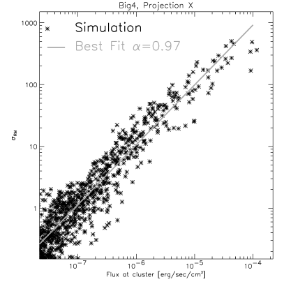
Figure 1: The symbols show a point by point comparison of the X-ray surface brightness and the RMS of the synthetic rotation measure calculated from one projection of one simulated cluster taken from the “medium” models. Overlayed is the best fit power-law. Clear to see that the correlation follows closely a power-law with a slope around unity.

Our models predict the structure of the magnetic field in galaxy clusters within the assumed scenario. One prediction is, that the magnetic field decreases with increasing distance from the center. Therefore we can predict the statistics of the rotation measure within our models. Comparing this with the X-ray emission provides an opportunity to measure the distribution of the magnetic field in galaxy clusters. Two quantities are obtained from the models at different positions in the cluster: the X-ray flux calculated as line of sight integral over the emissivity within the energy range $[0.1,2.4]$keV, which translates to an X-ray surface brightness, and the root mean square (RMS) of the synthetic rotation measure (RM). To this aim, the synthetic maps are divided in 125kpc x 125kpc boxes, in which the RMS of the rotation measure and the mean of the X-ray flux are calculated (see Fig. 1). Here, we compare the two line of sight integrals

$$S_{x}\propto\int n_{\mathrm{e}}^{2}\;\sqrt{T}\;{\mathrm{d}}x\Longleftrightarrow\sigma_{\mathrm{RM}}\propto\int n_{\mathrm{e}}\;B_{\|}\;{\mathrm{d}}x$$ (1)

with each other. In comparing the two quantities, we obtain the correlation of magnetic field versus density, when neglecting the temperature dependence on the left side. Actually, the dependence of the X-ray emission on the temperature is even flatter than the square root between 1 and 10 keV due to line emission. For the ROSAT energy range (0.1-2.4 keV) the temperature dependence can be neglected. We find a clear correlation between rotation measure and X-ray flux in all our simulated clusters suggesting that the magnetic field is directly related to the gas density. Fitting this correlation by

$$\sigma_{\mathrm{RM}}=A\left(\frac{S_{x}}{10^{-5}\mathrm{erg}/\mathrm{cm}^{2}/\mathrm{s}}\right)^{\alpha},$$ (2)

the slope $\alpha$ somewhat depends on the cutoff in surface brightness and rotation measure, applied to the synthetic data. The cutoff was chosen to be $10^{-4}$ of the maximum found in the individual maps. The fits tend to give values slightly smaller than one, but all the individual correlations are still consistent with a slope of one.

Figure 2: In the left panel the fitted slope $\alpha$ of the $\sigma_{\mathrm{RM}}$-$S_{x}$-correlation as function of the cluster temperature is plotted. Here fits in all three projection directions of all twenty model clusters are shown. The symbols are plotted only for the “medium” models. The large symbols are the ten main clusters, the smaller symbols are the smaller objects mentioned before. The lines mark the average over the ten main clusters (bold line) and the average over all 20 objects (thin line). The right side shows the normalization $A$ of the correlation function of these power-law fits for the same models. The different lines are for different initial field configurations as labeled in the plot.

Figure 2 shows the results of the slope $\alpha$ for various cluster models and for different initial magnetic field configurations in our simulation. To increase the temperature range of clusters used for this analysis we also include the ten smaller objects found near the main clusters in our simulations as described before. In total we use twenty different objects for every initial magnetic field configuration, in which we analyze three spatial projection directions. The left panel of Fig. 2 shows that the slope of the correlation is constant over the temperature range of our simulations. The symbols are taken from the “medium” models, the different lines are the best fits to different magnetic field configurations as labeled in the plot. It is obvious that the slope did not change for different initial field strengths and orientations. The large symbols are the ten main clusters, the smaller symbols are the smaller objects. Also the clusters with doubled mass resolution show the same slope. There is a small trend visible, that when including the smaller objects, the slope tends to be somewhat smaller. This is only 5% and may well be due to the poor resolution in these smaller objects and due to the chosen cutoff for the fitting procedure. Also here, a slope of 1, yields a good fit to data. The obtained values for the fits to the synthetic data are summarized in Table 1.

The simulations not only predict that the magnetic field scales similarly to the density within all clusters but also show that clusters have different central magnetic field strengths depending on their dynamical state and their temperature, leading to an offset of this correlation. Therefore the normalization $A$ of the $\sigma_{\mathrm{RM}}$-$S_{x}$-correlation in Eq. 2 should depend on the “global” magnetic field strengths (determined in the simulations by choosing the initial field strengths), the temperature of the cluster and its dynamical state. Analyzing the whole set of clusters, we expect to see a trend of the normalization with cluster temperature, whereas the scatter around this trend should be due to the individual dynamical states of the clusters.

The right panel of Fig. 2 shows, as expected, that the normalization $A$ of this correlation rises with temperature and increasing “global” magnetic field strengths, but does not change for different field configurations or when doubling the mass resolution. The symbols are again taken from the “medium” models, the different lines are the best fit of

$$A\propto T^{\delta}$$ (3)

for all the different models as labeled in Fig. 2. The values obtained for these fits are also summarized in Table 1. The large scatter of the individual objects around this trend also suggests, that the dynamical state of the individual objects plays a crucial role. This reflects the established fact that merging of clusters strongly amplifies the magnetic field (Roettiger et al 1999). Table 1 (column 6) also summarize the calculated RMS of the individual clusters around this scaling of the normalization $A$.

4 Data Presentation

Table 2: Summary of cluster data used for the analysis

Cluster	z	Redshift	$n_{\mathrm{H}}$	Temperature	Temperature	Temperature
		reference	$[10^{21}]$	[keV]	reference	used
A119	0.0443	Struble & Rood (1999)	0.289	$5.1^{+1.0}_{-0.8}$	Edge et al. (1990)
				$5.9^{+1.1}_{-0.9}$	David et al. (1992)
				$5.6$	Markevitch et al. (1998)	X
A514	0.0714	Fadda et al. (1996)	0.321	$3.6^{*}$	Arnaud & Evrard (1999)
Coma	0.0232		0.0895	$8.2$	Arnaud et al. (2001)	X
3C129	0.021		7.1	$5.5\pm 0.2$	Leahy & Yin (2000)
				$5.6^{+0.7}_{-0.6}$	Edge & Steward (1991)	X
				$6.25^{+0.27}_{-0.26}$	Taylor et al. (2001)

Caption: Column 1: Cluster name; Column 2: Redshift; Column 3: Redshift reference; Column 4: $n_{\mathrm{H}}$ from Dickey & Lockman (1990); Column 5: Temperature; Column 6: Temperature reference; Column 7: Temperature used for the analysis; ^∗ derived from $L_{x}-T$ relation.

To analyze in detail the magnetic field structure in clusters of galaxies it is crucial to compare the correlation between the X-ray emission and the synthetic $\sigma_{\mathrm{RM}}$ with the relation obtained from the data.

For such a comparison we need highly polarized radio galaxies, located at different distances from the cluster center, for which the rotation measure and the contribution of the inter-galactic medium to the X-ray emissivity at the source position are known. The cluster A119 is the most important one for our analysis, as it contain three sources spanning a useful range of line of sights through the cluster. Additionally sources in A514, Coma and 3C129 are used for a combined analysis. Following, we give a brief description of the X-ray and radio data used here. While the radio data were taken from previous work, we re-analyzed X-ray archival data to measure the exact surface brightness at the position of the radio galaxies.

4.1 X-ray data

For the four clusters X-ray data obtained with ROSAT were retrieved from the archive. A 15 ksec ROSAT/PSPC observation was used for A119 in the hard band (0.5-2.0 keV). For A514 an 18 ksec ROSAT/PSPC observation (hard band) was used. The pointing contains many point sources which are probably not associated with the cluster. These point sources were removed before smoothing by replacing the pixel values with values taken from the surrounding area. For the Coma cluster we used a 21 ksec ROSAT/PSPC observation. Also here only the hard band data were taken into account. For 3C129 two ROSAT/HRI pointings were used with a total exposure time of 39 ksec. For all clusters the X-ray values were extracted from images with a Gaussian smoothing of $\sigma$=40^′′. The backgrounds were taken from empty regions in the pointings. For the cluster 3C129 the background is higher, because it is an HRI observation. This high background introduces a large uncertainty into the countrate of 3C129 of about 50%. For the other clusters the errors in the countrate are statistical errors inferred from the numbers of photons observed at the position of the radio sources. For the source in the Coma cluster additionally note that the X-ray flux over the region of the radio source varies by $\pm 5$%. This variation is taken into account in the error listed in Table LABEL:tab1.

A summary of the clusters we used can be found in Table LABEL:tab_cl. Note that for some clusters different temperatures are given in literature. As no good temperature measurement exists for A514 the temperature was estimated from the $L_{x}-T$ relation (Arnaud & Evrard 1999).

4.2 Radio data

Table 3: Summary of RM and X-Ray data

Cluster	Radio source	Dist	$<$RM$>$	$\sigma_{\mathrm{RM}}$	X-ray (PSPC)	Background	Flux
		′	rad m-2	rad m-2	$10^{-3}$(cts/sec/arcmin2)	$10^{-3}$(cts/sec/arcmin2)	$10^{-5}$(erg/sec/cm2)
A119	0053-015	2.4	+28	$152^{+30}_{-42}$	$7.3\pm 0.6$	0.27	$2.4\pm 0.19$
′′	0053-016	6.4	-79	$91^{+20}_{-33}$	$4.0\pm 0.5$	′′	$1.3\pm 0.14$
′′	3C29	21.4	+4	$13^{+14}_{-13}$	$0.8\pm 0.2$	′′	$0.26\pm 0.07$
A514	J0448-2025	2.7	+104	$63^{+16}_{-41}$	$2.43\pm 0.31$	0.19	$0.86\pm 0.12$
′′	J0448-2032	7	+46	$47^{+11}_{-21}$	$2.09\pm 0.30$	′′	$0.76\pm 0.10$
′′	J0448-2032-N∗	6.6	+25	$54^{+12}_{-21}$	$2.26\pm 0.30$	′′	$0.82\pm 0.11$
′′	J0448-2032-S∗	7.3	+56	$38^{+10}_{-23}$	$2.04\pm 0.29$	′′	$0.74\pm 0.10$
3C129¶	3C129.1	0	+21	$200^{+39}_{-50}$	$2.25\pm 0.32$	3.5	$7.0\pm 1.0$
′′	3C129	16	-125	$82^{+17}_{-25}$	$0.73\pm 0.28$	′′	$2.3\pm 0.9$
Coma	NGC4869	5	-243	$87^{+36}_{-48}$	$25.4\pm 2.7$	0.69	$5.95\pm 0.6$

Caption. Column 1: Cluster name; Column 2: Source name; Column 3: Distance from the cluster center; Column 4: Average value of RM; Column 5: RM dispersion; Column 6: X-ray surface brightness in the ROSAT hard band, background corrected; Column 7: X-ray background used; Column 8: X-ray flux at the position of the radio source; ^∗Source divided into North and South lobe; ^¶ HRI counts;

The rotation measures of the radio sources in A119, A514, Coma and 3C129 have been obtained with the Very Large Array (VLA), using sensitive data at multiple wavelengths.

Linear polarized electromagnetic radiation passing through a magnetized ionized medium suffers a rotation of the plane of polarization:

$$\Psi(\lambda)=\Psi_{0}+\lambda^{2}RM$$ (4)

where $\Psi(\lambda)$ is the position angle observed at a wavelength $\lambda$ and the $\Psi_{0}$ is the intrinsic position angle. The position angle of the plane of polarization is an observable quantity, therefore, images of rotation measure can be constructed, by linear fitting the polarization angle as a function of $\lambda^{2}$.

In the cluster A119, the polarization properties of three extended radio galaxies were analyzed (Feretti et al. 1999). The two sources 0053-015 and 0053-016 show a head-tail structure of about 5′ in size, and are projected close to the cluster center, The third source, 3C29 (0055-016), is a typical FRI, about 2.5′  in size and located at the cluster periphery. In the cluster A514, two extended radio sources are suitable for a polarization study (Govoni et al., in preparation), owing to their high degree of polarization: J0448-2025 is a head-tail radio source of about 0.8′  in size while J0448-2032 is an FRI radio galaxies with an projected extension of about 1.4′. In the Coma cluster, the tailed radio galaxy NGC4869 was analyzed by Feretti et al. (1995). It is located near the cluster center and it is extended about 4′. In the 3C129 cluster, two radio sources were analyzed by Taylor et al. (2001): 3C129.1 at the cluster center, and the tailed radio galaxy 3C129 at the cluster periphery.

To estimate the errors on the dispersion of the rotation measure, we assumed the $\sigma_{\mathrm{RM}}$ composed as follows:

$$(\sigma_{\mathrm{RM}})^{2} = (\sigma_{\mathrm{RM}}^{\mathrm{measured}})^{2}-(1\pm\eta_{1})(\sigma_{\mathrm{RM}}^{\mathrm{noise}})^{2}$$ (5)

$$\pm 2\sigma_{\mathrm{RM}}^{\mathrm{measured}}\sigma_{\mathrm{RM}}^{\mathrm{noise}}/\sqrt{N}$$

$$\pm \eta_{2}(\sigma_{\mathrm{RM}}^{\mathrm{measured}})^{2}.$$

Here, the first term $\sigma_{\mathrm{RM}}^{\mathrm{measured}}$ is the signal extracted from the map. The second term describes the widening of the signal due to the uncertainties $\sigma_{\mathrm{RM}}^{\mathrm{noise}}$ within the individual pixels of the maps, where $\eta_{1}$ reflects our lack of knowledge of this value. We chose $\sigma_{\mathrm{RM}}^{\mathrm{noise}}$ between 20 and 30 for the individual maps and a value of 0.5 for $\eta_{1}$, as these errors are not known very precisely. The third term reflects the statistical error inferring $\sigma_{\mathrm{RM}}^{\mathrm{measured}}$ from the given distribution of $N$ independent resolution elements across the source and is small due to the fact that $N$ is moderately high. The last term reflects the uncertainty of the exact source position along the line of sight, characterized by the value of K in Eq. (9). We chose $\eta_{2}=(624-411)/411=0.52$ as the typical value. Note that in principle the fourth term only contributes when the rotation measure is deprojected.

For each radio source, Table LABEL:tab1 shows the distance from the cluster center, the average value of the RM, the $\sigma_{\mathrm{RM}}$, the X-ray surface brightness, X-ray background and the X-ray flux of the cluster calculated in the position of the radio source. In both clusters, A119 and A514, the value of the $\sigma_{\mathrm{RM}}$ decreases with increasing projected distance from the cluster center. These data are good evidence for the existence of a magnetic field associated with the intra-cluster medium which contributes to the Faraday rotation according to how much magneto-ionized medium is crossed by the polarized emission.

4.3 Modeling the magnetic field

Various physical models have been invoked to explain the rotation measures observed in radio sources belonging to clusters of galaxies (Lawler & Dennison 1982, Tribble 1991, Felten 1996).

Assuming a magnetic field topology with cells of constant size, density and magnetic field strength, but random orientation inside each cell, the contribution to the RM from each cell is given by:

$$RM=812n_{e}B_{\parallel}l\leavevmode\nobreak\ \leavevmode\nobreak\ \leavevmode\nobreak\ (rad\leavevmode\nobreak\ m^{-2})$$ (6)

where $n_{e}$ is the electron density in cm^-3, $B_{\parallel}$ is the magnetic field component along the line of sight measured in $\mu$G, and $l$ is the cell size in kpc. The observed RM, along any given line of sight, will be generated by a random walk process. Thus, the distribution of RM can be modeled with a Gaussian with mean value of 0 ($rad\leavevmode\nobreak\ m^{-2}$) and dispersion given by:

$$\sigma_{\mathrm{RM}}=\frac{812}{\sqrt{3}}n_{e}BN^{\frac{1}{2}}l$$ (7)

where N is the number of cells along the line of sight.

Considering a similar model but with a density distribution that follows a $\beta$-profile:

$$n_{e}(r)=n_{0}(1+r^{2}/r^{2}_{\rm c})^{-3\beta/2}$$ (8)

where $n_{0}$ is the central gas density, $r_{\rm c}$ is the core radius, and $\beta$ is the slope of the profile, Felten (1996) derived the following relation for the RM dispersion:

$$\sigma_{\mathrm{RM}}={{KBn_{0}r_{c}^{1/2}l^{1/2}}\over{(1+r^{2}/r_{c}^{2})^{(6\beta-1)/4}}}\sqrt{{\Gamma(3\beta-0.5)}\over{\Gamma(3\beta)}}$$ (9)

where $\Gamma$ is the Gamma function (while the other parameters have the same meaning as in the previous formula). The factor $K$ depends on the integration path over the gas density distribution: $K$ = 624, if the source lies completely beyond the cluster, and $K$ = 441 if the source lies at the cluster center.

By combining Eq. (9) with the X-ray surface brightness profile obtained from a $\beta$ model:

$$S(r)=S_{0}(1+r^{2}/r_{c}^{2})^{-3\beta+0.5}$$ (10)

and assuming that the factor $K$ is the same for all sources in a cluster, we expect a power-law correlation between the $\sigma_{\mathrm{RM}}$ and the X-ray brightness with an index $\alpha$=0.5. This slope of the correlation is independent of the values fitted for $\beta$ and $r_{\rm c}$. This expected relation, obtained assuming a constant magnetic field and cell size is plotted in Fig. 3 as a solid line.

5 Comparing observations

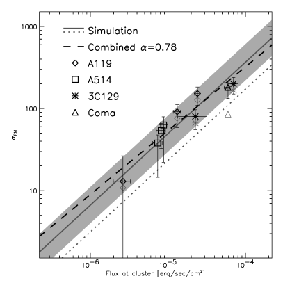
Figure 3: Shown is the measured correlation between the X-ray surface brightness and the RMS of the rotation measurement (left panel). The symbols are the measurements from the clusters as indicated in the plot. For 3C129 the HRI counts are converted to PSPC hard band counts with a factor of 2.4. The dashed and the dotted line show the best fit to the individual clusters A119 and 3C129. The solid line shows the expected correlation for an overall constant magnetic field inside the cluster adapted to the data from A119. The right panel combines all measurements by converting the surface brightness to the position of the cluster. The expected correlation for a 5keV cluster from the simulations is shown for the “high” models (solid line) and for the “medium” model (dotted line). The gray region marks the scatter for individual clusters expected for the simulations of the “high” models. The combined fit to the data is shown as dashed line. The gray symbols indicate, where the data points move when we correct for the cluster temperature according to the theoretical models.

In order to test whether the correlation found in model clusters is also present in real clusters we use observational radio and X-ray data. In principle, each cluster with enough radio source polarization measurements would allow us to determine the correlation between $S_{x}$ and $\sigma_{\mathrm{RM}}$ individually and therefore give independent estimates, how the magnetic field scales with density in these objects. As there are only a small number of observations, even spread over several clusters, a combined analysis of these clusters is necessary. Once there are enough measurements their combined analysis could tell, how the magnetic field scales with the cluster temperature.

5.1 The observed $\sigma_{\mathrm{RM}}$-S_x correlation

The values for the individual sources within the clusters like positions, X-ray counts and RM measurements can be found in Table LABEL:tab1. In the left panel of Fig. 3 we show all data points drawn from our clusters. Plotted is $\sigma_{\mathrm{RM}}$ versus the X-ray surface brightness. Here we can try to fit the correlation in the individual clusters as indicated in the plot. The surface brightness is background corrected. The absorption plays no role for the slope calculated for the individual clusters as the counts for all sources within one cluster would have to be multiplied by the same value, leading only to a shift of this correlation. A119 (diamonds) has the best individual data, and the best fit relation gives a slope of $\alpha=1.13$ which is comparable to what we expect from the simulations. In 3C129 the lower data point has a large uncertainty in the X-ray measurement, as it is noise dominated. The correlation referred from these two data points gives a slope of 0.81, which is to within the uncertainties also consistent with the expectation from the simulations. The three data points for A514 are too close to infer seriously a slope, but they also suggest a slope larger than one i.e. far from the $\alpha=0.5$ slope for the simple models. For Coma (triangle) only one data point is available, therefore it can only be used in the combined analysis. For comparison a line with the slope of 0.5 is added as solid line. The amplitude is chosen such that it matches the innermost data point of A119, which has the highest values and therefore is the most reliable data point. Due to the lack of data, only A119 and marginally 3C129 allows us to determine the correlation from individual clusters, but both show consistently that the slope in real clusters is close to the expected slope from the simulations, rather than the expected slope of oversimplified models.

5.2 Fitting the combined Data

For combining all measurements we have to convert the X-ray measurements to quantities at the clusters themselves to be independent of distance and absorption. To be able to compare them with the simulations, we chose to convert the surface brightness to the position of the cluster taking into account the distance, the cluster temperature and the absorption by Galactic hydrogen $n_{\rm H}$. The values we used for the clusters can be found in Table LABEL:tab_cl, where column 7 marks which of the different temperatures for individual clusters we have chosen from literature. The calculated flux for the individual sources can be found in Table LABEL:tab1. The results are shown in the right panel of Fig. 3 (thick symbols).

The gray solid line represents the expected correlation for a simulated 5keV cluster taken from the “high” models. The gray region marks the expected RMS for individual clusters around this prediction, as given in the last column of Table 1. The dotted line is the expected correlation for a 5keV cluster taken from the “medium” models. Taking the shift of the correlation with cluster temperature within the “medium” model, the solid line would represent an 8keV cluster.

All measurements combined follow very well the correlation expected from the simulations. The combined fit gives a marginally smaller slope of 0.78 (dashed line), but the data are still incompatible with a slope of 0.5.

Suggested by the simulations, we have to take into account a possible scaling of the magnetic field with cluster temperature when we want to combine the measurements from individual clusters. In the case of enough measurements, the combined data could be used to infer how the magnetic field in different clusters scales with their temperature by looking for the scaling which leads to the smallest scatter in the combined correlation. With the limited data currently available, we can only sketch how to apply the calibration of this correlation, according to the theoretical models. As previously found (see Fig. 2), the normalization of this correlation scales as

$$A\propto\left(\frac{T}{5\mathrm{keV}}\right)^{\delta}.$$ (11)

As the value of $\delta$ changes with the magnetic field model used in the simulations, we took a $\delta=1.6$ from the “medium” model, but the difference when taking the slightly different slopes from the other models is marginal. As all clusters have measured temperatures larger than 5keV this calibration shifts the data points towards lower rotation measure shown as thin, gray symbols in Fig. 3. For A514 there is no direct measurement for the temperature, only an estimate for the temperature from the $L_{x}-T$-relation. Therefore we did not apply the correction to A514.

As the source within Coma is the only data point, which is significantly changed when applying the theoretical correction, it is not possible to test really if the magnetic field changes with cluster temperature. When correcting for temperature according to the simulations, the RMS measurement for Coma drops somewhat below the expected correlation. As this is only one data point, and we expect a large scatter from the simulations. This lies within the expectations, and no definite conclusion could be drawn from the data available at the moment.

The combined measurements follow the theoretical expectation from our simulations very well. This holds for the individual clusters as well as for the combined measurements. If we take the small number of available data into account, the differences between the fits for individual clusters themselves, the combined measurements and the simulations are very small. They also indicate, that the slope of unity inferred from the simulations is clearly favored by the data with respect to a slope of 0.5 inferred from simple models. The comparison of the observed $\sigma_{\mathrm{RM}}$-$S_{x}$ correlation with the simulations shows, that a magnetic field somewhere between the “medium” and “high” models reproduces the observations best.

5.3 Implication on measuring the magnetic field B

We can extend the modeling of the magnetic field in Sect 4.3 to the case of variable magnetic field within the cluster. Assuming, that the magnetic field $B$ scales with the density $n_{e}$ as

$$B\propto(n_{e})^{\gamma},$$ (12)

$\beta$ in Eq. (9) must be replaced by $\beta(1+\gamma)$. Combining this modified Eq. (9) with (10) yields the slope of the $\sigma_{\mathrm{RM}}$-S_x correlation to be

$$\alpha=0.5\frac{3\beta(1+\gamma)-0.5}{3\beta-0.5}$$ (13)

with $\gamma$ being the slope of the B-n_e relation. For a constant magnetic field ($\gamma=0$) this yields an index of $\alpha$=0.5, independent of the values of $\beta$ and $r_{\rm c}$, as already shown in Sect. 4.3. The lines in Fig. 4 allow for a direct inference of the B-n_e slope $\gamma$ for measured $\alpha$ and $\beta$. Assuming $\beta=0.7$ one finds a $\gamma$ between 0.5 and 0.9 for the observed slopes $\alpha$ between 0.8 and 1.1. This is still a simplified model, as a constant scale length is assumed.

Figure 4: Conversion of the slope of the $\sigma_{\mathrm{RM}}$-S_x correlation $\alpha$ to the slope of the B-n_e relation $\gamma$ for given values of the X-ray profile shape parameter $\beta$. The parameters of A119, $\alpha$=1.13 and $\beta$=0.56 (shown as diamond), a value for $\gamma$ of 0.9 is inferred.

For A119 a $\beta$=0.56 is obtained from the X-ray data and a slope $\alpha$=1.13 is derived from the fit to the $\sigma_{\mathrm{RM}}$-S_x correlation (see Fig. 3). These values yields a $\gamma=0.9$. For a cell size of 10-20kpc Feretti et al. (1999) calculated a magnetic field $\approx 5\mu$G using the constant magnetic field approximation. Taking into account the model allowing for a varying magnetic field we obtain a central magnetic field of $\approx 7.5\mu$G, which decreases with radius according to $(n_{e})^{0.9}$.

For 3C129 a $\beta=0.47$ is measured (Taylor et al. 2001) and we infer a slope $\alpha=0.81$ from drawing a line through the two points of the $\sigma_{\mathrm{RM}}$-S_x correlation (see Fig. 3). This results in a $\gamma=0.5$, but – due to the poor X-ray data of the lower data point – this value has a large uncertainty.

6 Conclusions

We find a correlation between the magnetic field and the intracluster gas density in galaxy clusters both, in our MHD simulations and in observational data taken from literature. The results rule out a magnetic field that is constant within a cluster. Instead we find in the simulations a correlation between the RMS of rotation measure and the X-ray emission in galaxy clusters with a slope of 1. Using all observational data currently available, we show that this correlation is indeed observed in individual clusters, in particular in A119, where the observations show a slope close to unity.

The combination of the measurements of 4 clusters suggests that this correlation is likely to be universal. The analysis of the combined data leads to a slightly lower slope of this correlation ($\alpha$=0.8), which may be due to the expected scatter between individual clusters, but is still compatible with the simulations and certainly excludes an overall constant magnetic field.

The observational quantities, rotation measure and X-ray flux, can be transformed to the physical quantities, magnetic field and intra-cluster gas density, with the help of the $\beta$-model. The relation between the slopes (Eq. 13) yields $B\propto n_{e}^{\gamma}$ with $\gamma=0.9$ for A119. For 3C129 we infer a $\gamma=0.5$ with large uncertainty.

Unfortunately, with the limited measurements presently available, it is not possible to infer if and how the magnetic field in different clusters depends on other cluster properties like temperature.

- (1) Allen S. W., Taylor G. B., Nulsen, P. E.J., et al., 2001, MNRAS 324, 842
- (2) Arnaud, M., Aghanim, N., Gastaud, R., Neumann, D. M., Lumb, D., et al. 2001, A&A, 365, L67
- (3) Arnaud M., Evrard A.E., 1999, MNRAS 305, 631
- (4) Bagchi J., Pislar V., Lima Neto G.B., 1998, MNRAS 296, L23
- (5) Bartelmann, M., Steinmetz, M., 1996, MNRAS, 283, 431-446
- (6) Blasi P., Burles S., Olinto A.V., 1999, ApJ 514, L79
- (7) Brunetti G., Setti G., Feretti L., Giovannini G., 2001, MNRAS 320, 365
- (8) Clarke T.E., Kronberg P.P., Böhringer H., 2001, ApJ 547, L111
- (9) De Young D.S., 1992, ApJ 386, 464
- (10) Dickey, J. M., and Lockman, F. J. 1990, Ann. Rev. Astron. Astrophys., 28, 215
- (11) Dolag, K., 2000, in: Constructing the Universe with Clusters of Galaxies, IAP 2000 meeting, Paris, France, Florence Durret & Daniel Gerbal Eds., http://www.iap.fr/Conferences/Colloque/coll2000/contributions
- (12) Dolag K., Bartelmann M., Lesch H., 1999, A&A 348, 351
- (13) Dreher J.W., Carilli C.L., Perley R.A., 1987, ApJ 316, 611
- (14) Fadda D., Girardi M., Giuricin G., et al., 1996, ApJ 473, 670
- (15) Felten J.E., 1996, In: Clusters, Lensing, and the Future of the Universe, ASP Conference Series, Vol. 88, Eds. V.Trimble and A.Reisenegger, p. 271
- (16) Feretti L., 1999, in Diffuse Thermal and Relativistic Plasma in Galaxy Clusters, Eds. H. Böhringer, L. Feretti & P. Schuecker, MPE Report n. 271, MPE Garching, p. 3
- (17) Feretti L., Dallacasa D., Giovannini G., Tagliani A., 1995, A&A 302, 680
- (18) Feretti L., Dallacasa D., Govoni F., Giovannini G., Taylor G.B., Klein U., 1999, A&A 344, 472
- (19) Fusco-Femiano R., Dal Fiume D., Feretti L., et al., 1999, ApJ 513, L21
- (20) Fusco-Femiano R., Dal Fiume D., De Grandi S., et al., 2000, ApJ 534, L10
- (21) Giovannini G., Feretti L., Stanghellini C., 1991, A&A 252, 528
- (22) Giovannini G., Feretti L., Venturi T., Kim K.-T., Kronberg P.P., 1993, ApJ 406, 399
- (23) Godon P., Soker N., White R. E. III, 1998, ApJ 116, 37
- (24) Goldshmidt O., Rephaeli Y, 1993, ApJ 411, 518
- (25) Ito, T., Makino, J., Fukushige, T., Ebisuzaki, T., Okumura, S.K., Sugimoto, D., 1993, PASJ, 45, 339
- (26) Jaffe W.J., 1980, ApJ 241, 925
- (27) Kim K.T., Tribble P.C., Kronberg P.P., 1991, ApJ 379, 80
- (28) Kronberg P.P., 1994, Rep. Prog. Phys. 325, 382
- (29) Kronberg P.P, Lesch H.,, Lepp U., 1999, ApJ 511, 56
- (30) Lawler J.M., Dennison B., 1982, ApJ 252, 81
- (31) Olinto A., 1997, in 3rd RESCEU International Symposium on “Particle Cosmology”, Tokyo, astro/ph-9807051
- (32) Pudritz R.E., Silk J., 1989, ApJ 342, 650
- (33) Rephaeli Y., Gruber D., Blanco P., 1999, ApJ 511, 21
- (34) Roettiger, K., Stone, J.M., Burns, J.O., 1999, ApJ, 518, 594
- (35) Ruzmaikin A., Sokoloff D., Shukurov A., 1989, MNRAS 241, 1
- (36) Soker N., Sarazin C.L., 1990, ApJ 348, 73
- (37) Struble M.F., Rood H.J., 1999, ApJS 125, 35
- (38) Taylor G.B., Perley R.A., 1993, ApJ 416, 554
- (39) Taylor G.B., Govoni F., Allen S.A., Fabian A.C., 2001, MNRAS in press, astro-ph/0104223
- (40) Tribble P.C., 1993, MNRAS 263, 31
- (41) Tribble P.C., 1991, MNRAS 250,726
- (42) Völk H.J., Atoyan A.M., 1999, Astrop. Phys. 1, 73