A Solution to the Missing Link in the Press-Schechter Formalism

Abstract

The Press-Schechter (PS) formalism for mass functions of the gravitationally collapsed objects is reanalyzed. It has been suggested by many authors that the PS mass function agrees well with the mass function given by $N$-body simulations, while many too simple assumptions are contained in the formalism. In order to understand why the PS formalism works well we consider the following three effects on the mass function: the filtering effect of the density fluctuation field, the peak ansatz in which objects collapse around density maxima, and the spatial correlation of density contrasts within a region of a collapsing halo because objects have non-zero finite volume. According to the method given by Yano, Nagashima & Gouda (YNG) who used an integral formula proposed by Jedamzik, we resolve the missing link in the PS formalism, taking into account the three effects. While YNG showed that the effect of the spatial correlation alters the original PS mass function, in this paper, we show that the filtering effect almost cancels out the effect of the spatial correlation and that the original PS is almost recovered by combining these two effects, particularly in the case of the top-hat filter. On the other hand, as for the peak ansatz, the resultant mass functions are changed dramatically and not in agreement especially at low-mass tails in the cases of the Gaussian and the sharp $k$-space filters. We show that these properties of the mass function can be interpreted in terms of the kernel probability $P(M_{1}|M_{2})$ in the integral formula qualitatively.

NAOJ-Th-Ap2001, No.44

1 Introduction

It is one of the most important work to determine the number density of collapsed objects from the statistical properties of the density fluctuation field at an early stage of cosmic structure evolution. Such number density, or the mass function of halos, constitutes a main body of analyses of cosmic structures such as galaxies. The pioneering work was done by Press & Schechter (1974, hereafter PS). They derived a mass function by relating a one-point distribution function of density fluctuation with a multiplicity function of halos. It is very simple and useful, and therefore has been applied to many problems related with statistics of cosmic objects by many authors. Moreover, in order to take into account the formation histories of galaxies, it has been extended to estimate the mass function of progenitors of a present-day halo (Bower 1991; Bond et al. 1991, hereafter BCEK; Lacey & Cole 1993, hereafter LC; Kauffmann & White 1993; Somerville & Kolatt 1998). Thus to remove uncertainties in the PS formalism and to refine it are very important.

Recent understanding on the cosmological structure formation is based on a cold dark matter (CDM) model which is a kind of the hierarchical clustering scenario. In the CDM model, the Universe is dominated by a cold dark matter gravitationally, and the self-gravitating structures are formed via a gravitational growth of small initial density fluctuations. Since higher density regions collapses earlier and since the power at smaller scales of the fluctuations is stronger than that at larger scales, larger objects which are formed by collapse of large-scale fluctuations are formed by clustering of smaller objects hierarchically. Formation processes of objects such as galaxies and galaxy clusters are qualitatively well understood in the context of such hierarchical clustering scenario. However, once we would like quantitative estimate, especially in regard with the statistical properties such as luminosity function of galaxies and abundance of clusters of galaxies, we face on difficulties caused by uncertainties to estimate the mass function of cosmological objects.

The PS formalism is the most useful even at present. This formula assumes a Gaussian distribution of density contrast and spherically symmetric collapse of objects (briefly reviewed in §2). In the PS formalism, however, there is a problem of the so-called “fudge-factor-of-two”. Because their consideration was only in overdense regions, they simply multiplied the factor of two in order to consider all matter in the Universe.

Another approach explaining the distribution of cosmological structures has been developed, that is, the peak formalism. This was firstly investigated by Doroshkevich (1970), and extensively studied by Peacock & Heavens (1985) and Bardeen et al. (1986, hereafter BBKS). In this formula, considering configurations of local density maxima through the first and second derivatives of the density fluctuation, the number density of the density peaks is derived. However, peaks in a field with larger smoothing scale often include those with smaller smoothing scale. Thus the mass function derived from the peak formalism is in agreement with numerical experiments only at very large mass scales (Appel & Jones 1990). In order to derive a correct mass function, we must remove such small scale peaks contained in larger peaks (the so-called cloud-in-cloud problem). By using “the confluent system formalism”, Manrique & Salvador-Solé (1995) derived a mass function taking into account the removal of nested peaks in the case of a Gaussian filter.

Peacock & Heavens (1990; hereafter PH90) and BCEK attempted to solve the cloud-in-cloud problem by considering a trajectory of a density fluctuation against the varying smoothing scale. The method is called the excursion set formalism according to BCEK. Assuming the spherical collapse, the threshold for the collapse is determined by only the value of the density fluctuation, independent of mass scale. Thus we adopt as a mass scale of the density fluctuation of a viriallized object, a maximum mass scale at which the density contrast is firstly upcrossing the threshold for decreasing mass scale. When the sharp $k$-space filter is adopted, they obtained the fudge-factor-of-two because of the Brownian motion of the trajectories due to uncorrelativity of phases of Fourier modes. However in the case of general filters, since the correlation between different Fourier modes originates the non-Markov behavior, a Monte Carlo method or complicated approximations are required, as done by PH90 and BCEK. It should be noted that this problem had already been considered by Epstein (1983; 1984) in the case of a Poisson fluctuation of point masses.

In contrast to the excursion set formalism, which is based on a differential formula such as the diffusion equation, Jedamzik (1995) proposed another approach based on an integral equation. YNG fixed an inconsistency of estimation of probability in the original analysis by Jedamzik (1995) and also obtained the fudge-factor-of-two in the case of the sharp $k$-space filter. While within the case of the sharp $k$-space filter, they extended the Jedamzik’s integral formula to include the effect of the spatial correlation which should be considered within a collapsing region in order to solve the cloud-in-cloud problem. They found that the factor of two is lost by the spatial correlation and predicted larger number density of halos compared to the PS mass function at large scale at which the variance of the density fluctuation becomes below unity. They also connected the peak formalism with the Jedamzik formula and found that the low-mass tail of mass function is changed. Nagashima & Gouda (1997) confirmed that the mass function given by YNG is in agreement with that given by the Merging Cell model proposed by Rodrigues & Thomas (1996), in which the density fluctuation field is realized by Monte Carlo method and halos are identified according to the linear theory and the spherical collapse model.

On the other hand, Monaco (1995; 1997a, b;1998) investigated the dynamical effect of the collapse by using nonlinear dynamics such as the Zel’dovich approximation (Zel’dovich 1970). As well known, the critical density contrast is 1.69 independent of mass scale for the spherical collapse in the Einstein-de Sitter universe. However, the probability finding objects collapsing spherically is very small and most of halos collapse non-spherically. Taking into account such direction-dependent dynamics, if we interpret a first shell-crossing epoch as a collapsing epoch, it was found that the resultant mass function is similar to the PS mass function with effectively decreased critical density below 1.69.

The purpose of this paper is to clarify why the PS mass function works well and well reproduces mass functions obtained by $N$-body simulations (e.g., Sheth & Tormen 1999; Jenkins et al. 2001). Hereafter we call this problem the missing link in the PS formalism. In this paper we consider the following three effects based on the integral formula developed by Jedamzik (1995) and YNG. First the filtering effect is investigated. We use the sharp $k$-space, the Gaussian, and the top-hat filters. Second the peak effect is considered, based on the peak ansatz in which objects collapse around density maxima. Third the spatial correlation is introduced in the same way as YNG, but for the above three filters. Finally all the effects are considered simultaneously. Since it is very complicated that the dynamical effect as considered by Monaco is introduced simultaneously, we will only discuss this effect in §6.

The structure of this paper is as follows. First in §2, we define the smoothed density field introducing the filters. In §3, we review the PS formalism. In §4, we show the formulation by using an integral equation, based on Jedamzik (1995) and YNG. In §5, we show the resulting mass functions and consider the effects of the filters, peaks, and spatial correlation. In §6 we discuss some uncertainties which we do not investigate in detail. We devote §7 to summary and conclusions. Many detailed definitions and equations are summarized in Appendix.

2 Smoothed Gaussian Random Field

First, we define the density contrast as $\delta({\bf x})\equiv\frac{\rho({\bf x})-\bar{\rho}}{\bar{\rho}}$, where $\rho({\bf x})$ is the density at the point ${\bf x}$ and $\bar{\rho}$ is the cosmic mean density. The Fourier mode of the density contrast, $\delta_{\bf k}$, is obtained by

$$\delta_{\bf k}=\int\delta({\bf x})e^{i{\bf k\cdot x}}d{\bf x}.$$ (1)

This density contrast is smoothed out by a window function $W_{M}(r)$ with a smoothing mass-scale $M$,

$$\delta_{M}({\bf x}) \equiv \int W_{M}(|{\bf x^{\prime}-x}|)\delta({\bf x^{\prime}})d{\bf x^{\prime}}$$ (2)

$$= \frac{1}{(2\pi)^{3}}\int{\tilde{W}}(kR)\delta_{\bf k}{e^{-i{\bf k\cdot x}}}d{\bf k},$$ (3)

where ${\tilde{W}}(kR)$ is the Fourier transform of the window function, $W_{M}(r)$, $R$ is a scale related to the mass $M$, and $k\equiv|{\bf k}|$.

The following three filters are often used as the window function by using the smoothing length $R$:

1. Top-hat filter
   

   $$W_{M}(r) = \frac{3}{4\pi R^{3}}\theta(1-\frac{r}{R}),$$ (4)

   $${\tilde{W}}(kR) = \frac{3}{(kR)^{3}}(\sin kR-kR\cos kR).$$ (5)

2. Gaussian filter
   

   $$W_{M}(r) = \frac{1}{(2\pi R^{2})^{3/2}}\exp\left(-\frac{r^{2}}{2R^{2}}\right),$$ (6)

   $${\tilde{W}}(kR) = \exp\left(-\frac{k^{2}R^{2}}{2}\right).$$ (7)

3. Sharp $k$-space filter
   

   $$W_{M}(r) = \frac{\sin k_{c}r-k_{c}r\cos k_{c}r}{2\pi^{2}r^{3}},$$ (8)

   $${\tilde{W}}(kR) = \theta(k_{c}-k),$$ (9)

where $k_{c}$ is the cut-off wave number, $k_{c}\simeq R^{-1}$, and $\theta(x)$ is the Heaviside step function.

Next we define a variance of the density field with a smoothing mass-scale $M$, $\sigma^{2}_{0}(M)$. The variance is obtained by using the power spectrum $P(k)\equiv\langle|\delta_{\bf k}|^{2}\rangle$ as follows,

$$\sigma^{2}_{0}(M)\equiv\langle\delta_{M}^{2}\rangle=\frac{1}{(2\pi)^{3}}\int{\tilde{W}}^{2}(kR)P(k)4\pi k^{2}dk.$$ (10)

The one-point distribution function in the Gaussian random field is characterized by the above variance. The normalization of the power spectrum is given by a characteristic mass $M_{*}$ at which $\sigma_{0}(M_{*})=1$.

In connection with the definition of $k_{c}$, here we define the mass $M$ with a scalelength $R$ or $k_{c}$. In the case of the top-hat filter, the mass $M$ is clearly related to $4\pi R^{3}\bar{\rho}/3$. On the other hand, for the other filters, the relation is not trivial. For example, LC proposed that the mass should be defined as the enclosed mass by the window function $W_{M}(r)$ renormalized to $W_{M}(r=0)=1$. It should be noted that this uncertainty does not emerge in the case of the Gaussian filter because it can be renormalized into $M_{*}$ in the case of the scale-free power spectrum. As for the sharp $k$-space filter, in this paper, we adopt a simple relation, $k_{c}R=\pi$, while LC adopted $k_{c}R=(9\pi/2)^{1/3}$. The $k_{c}-R$ relation will be discussed in §6.

By using the spherically symmetric collapse model (Tomita 1969; Gunn & Gott 1972), the critical density contrast $\delta_{c}$ is equal to 1.69 in the Einstein-de Sitter universe. So the region with $\delta\geq\delta_{c}$ is already included in a collapsed region. We adopt this value throughout this paper. Note that Monaco (1995) found that effective critical density contrast taking into account a non-spherical collapse is approximated as $\delta_{c}\simeq 1.5$ by dealing with $\delta_{c}$ as a free parameter and fitting the PS mass function to that given by him.

In the followings, we restrict ourselves to the Einstein-de Sitter cosmological model and scale-free power spectra, $P(k)\propto k^{n}$ with $n=0$ and $n=-2$, except for §§5.4 in which we will show mass functions in a CDM universe.

3 The Press-Schechter Formalism

In this section, we review the Press-Schechter formalism briefly. The probability of finding the region whose linear density contrast smoothed on the mass scale $M$, $\delta_{M}$, is greater than or equal to $\delta_{c}$ is assumed to be expressed by the Gaussian distribution given by

$$f(\geq\delta_{c};M)=\frac{1}{\sqrt{2\pi}\sigma_{0}(M)}\int_{\delta_{c}}^{\infty}\exp\left[-\frac{\delta^{2}}{2\sigma^{2}_{0}(M)}\right]d\delta.$$ (11)

This probability corresponds to the volume fraction of the region with more than or equal to $\delta_{c}$ in the density field with smoothing scale $M$ to the total volume in a fair sample of the Universe. Therefore, the difference between $f(\geq\delta_{c};M)$ and $f(\geq\delta_{c};M+dM)$ represents the volume fraction of the region for which $\delta_{M}=\delta_{c}$ precisely. The density contrast of an isolated collapsed object must be precisely equal to $\delta_{c}$ because an object with $\delta>\delta_{c}$ would be eventually counted as an object of larger mass scale. The volume of each object with mass scale $M$ is $M/{\bar{\rho}}$. Then we obtain the following relation,

$$\frac{Mn(M)}{\bar{\rho}}dM=-\frac{\partial f(\geq\delta_{c};M)}{\partial M}dM,$$ (12)

where $n(M)$ means the number density of objects with mass $M$, that is, the mass function. However, the underdense regions are not considered in the above equation. Hence, Press and Schechter simply multiply the number density by a factor of two,

$$\frac{Mn(M)}{\bar{\rho}}dM=-{\it 2}\frac{\partial f(>\delta_{c};M)}{\partial M}dM.$$ (13)

This factor of two has long been noted as a weak point in the PS formula (the so-called cloud-in-cloud problem). PH90 and BCEK proposed a solution to this problem by taking account the probability $P_{up}$ that a subsequent filtering of larger scales results in having $\delta>\delta_{c}$ at some point, even when at smaller filters, $\delta<\delta_{c}$ at the same point (the excursion set formalism). In the sharp $k$-space filter, because of the uncorrelation between different Fourier modes $\delta_{\bf k}$, the trajectory of $\delta_{M}$ behaves as a random walk for adding a new Fourier mode. In this case, they found that the factor of two in the PS formula is reproduced.

4 Integral equation approach

Jedamzik (1995) proposed another approach to the cloud-in-cloud problem based on an integral equation.

Now, we consider the regions whose smoothed linear density contrasts with smoothing mass scale $M_{1}$ are above $\delta_{c}$. Each region must be included in an isolated collapsed object with mass $M_{2}$ larger than or equal to $M_{1}$. Therefore, we obtain the following equation,

$$f(\geq\delta_{c};M_{1})=\int_{M_{1}}^{\infty}P(M_{1}|M_{2})\frac{M_{2}}{\bar{\rho}}n(M_{2})dM_{2},$$ (14)

where $P(M_{1}|M_{2})$ means the conditional probability of finding a region of mass scale $M_{1}$ in which $\delta_{M_{1}}$ is greater than or equal to $\delta_{c}$, provided it is included in an isolated overdense region of mass scale $M_{2}$. Hereafter we call the procedure in which the mass functions are estimated by solving eq.(14) the Jedamzik formalism. If $P(M_{1}|M_{2})$ is simply given by the conditional probability $p(\delta_{M_{1}}\geq\delta_{c}|\delta_{M_{2}}=\delta_{c})$, $P(M_{1}|M_{2})$ is written as follows by using the Bayes’ theorem,

$$P(M_{1}|M_{2}) = p(\delta_{M_{1}}\geq\delta_{c}|\delta_{M_{2}}=\delta_{c})$$ (15)

$$= \frac{1}{\sqrt{2\pi}\sigma_{{\rm sub}}}\int_{\delta_{c}}^{\infty}\exp\left\{-\frac{1}{2}\frac{(\delta_{M_{1}}-\delta_{c})^{2}}{\sigma^{2}_{{{\rm sub}}}}\right\}d\delta_{M_{1}}$$

$$= \frac{1}{2},$$

where $\sigma^{2}_{{\rm sub}}=\sigma^{2}_{0}(M_{1})-\sigma^{2}_{0}(M_{2})$ by using the sharp k-space filter. Thus we can obtain the PS formula, naturally including the factor of two as can be seen from eqs.(14) and (15). The reason originating the factor of two is a behavior of the random walk, and is essentially the same as the excursion set formalism.

However, it is insufficient to use eq.(15) for more realistic estimation of the mass function because it is necessary to consider the spatial correlation of the density fluctuations due to the finite size of objects. Besides the sharp $k$-space filter is used which leads $\sigma_{\rm sub}^{2}$ to $\sigma^{2}_{0}(M_{1})-\sigma^{2}_{0}(M_{2})$, then we should evaluate how the mass function is changed by other filters. Therefore, we must consider the probability $P(r,M_{1}|M_{2})$ of finding $\delta_{M_{1}}\geq\delta_{c}$ at a distance $r$ from the center of an isolated object of mass scale $M_{2}$ with general filters. Then we can get the probability $P(M_{1}|M_{2})$ by spatially averaging $P(r,M_{1}|M_{2})$.

Because we expect that the isolated collapsed objects are formed around density peaks, the constraints to obtain the above probability $P(r,M_{1}|M_{2})$ are given as follows:

1. The linear density contrast, $\delta_{M_{2}}$, of the larger mass scale $M_{2}$ should be equal to $\delta_{c}=1.69$ at the center of the object.

2. Each object of the mass scale $M_{2}$ must contain a maximum peak of the density field, i.e., the first derivative of the density contrast $\nabla\delta_{M_{2}}$ must be equal to $0$ and each diagonal component of the diagonalized Hessian matrix $\zeta$ of the second derivatives must be less than $0$ at the center of the object.

3. The density contrast of the smaller mass scale $M_{1}(\leq M_{2})$ which has been already collapsed and which is included in an object of mass scale $M_{2}$ must satisfy the condition $\delta_{M_{1}}\geq\delta_{c}$ at distance $r$ from the center of the larger object.

In order to evaluate the above conditions, in this paper, we investigate the following effects: (1) filters, (2) density peaks, and (3) spatial correlation. Some other effects will be discussed in §6.

5 Results

5.1 Filtering effect

In general filters except for the sharp $k$-space filter, the description of the Markovian random walk in the excursion set formalism cannot be adopted. PH90 and BCEK calculated the mass function by Monte Carlo method realizing Fourier modes $\delta_{\bf k}$ in such a non-Markov case. On the other hand, we can easily calculate the mass function by substituting the conditional probability in eq. (15) to general cases as a simple approximation. It is adequate approximation for the purpose of this paper in order to understand the various effects mentioned above, at least, qualitatively.

For this purpose, what we do is to estimate the probability,

$$P(M_{1}|M_{2})=p(\delta_{M_{1}}\geq\delta_{c}|\delta_{M_{2}}=\delta_{c}).$$ (16)

Note that in the case of general filters, we cannot reduce this probability to a half because of the correlation between the Fourier modes. Here we define the normalized density contrasts,

$$\nu_{1} \equiv \frac{\delta_{M_{1}}}{\sigma_{r}},$$ (17)

$$\nu_{2} \equiv \frac{\delta_{M_{2}}}{\sigma_{0}},$$ (18)

where the standard deviations $\sigma_{r}$ and $\sigma_{0}$ are the root mean squares of the variances $\langle\delta_{M_{1}}^{2}\rangle^{1/2}$ and $\langle\delta_{M_{1}}^{2}\rangle^{1/2}$, which are defined in Appendix A. Hereafter we refer values concerning $\delta_{M_{1}}$ to the subscript $r$.

Generally bivariate Gaussian distribution is given by

$$p(\nu_{1},\nu_{2}){\rm d}\nu_{1}{\rm d}\nu_{2}=\frac{1}{2\pi\sqrt{1-\epsilon^{2}}}\exp\left\{-\frac{(\nu_{1}-\epsilon\nu_{2})^{2}}{2(1-\epsilon^{2})}-\frac{\nu_{2}^{2}}{2}\right\}{\rm d}\nu_{1}{\rm d}\nu_{2},$$ (19)

where the correlation coefficient $\epsilon$ is equal to $\langle\nu_{1}\nu_{2}\rangle=\xi_{0}(0)/\sigma_{r}\sigma_{0}$, which is defined in Appendix A. The conditional probability distribution function is obtained by the Bayes’ theorem,

$$p(\nu_{1}|\nu_{2}=\nu_{2c}){\rm d}\nu_{1}=\frac{p(\nu_{1},\nu_{2c})}{p(\nu_{2c})}d\nu_{1}$$ (20)

$$= \frac{1}{\sqrt{2\pi(1-\epsilon^{2})}}\exp\left\{-\frac{(\nu_{1}-\epsilon\nu_{2c})^{2}}{2(1-\epsilon^{2})}\right\}{\rm d}\nu_{1},$$

where $\nu_{2c}$ is the normalized critical density contrast with the smoothing scale $M_{2}$, $\delta_{c}/\sigma_{0}$, and $p(\nu)$ is a one-point Gaussian normal distribution,

$$p(\nu)d\nu=\frac{1}{\sqrt{2\pi}}\exp\left(-\frac{\nu^{2}}{2}\right)d\nu.$$ (21)

In the case of the sharp $k$-space filter, the covariance $\xi_{0}(0)$ is reduced to $\sigma_{0}^{2}$, then we obtain $\epsilon=\sigma_{0}/\sigma_{r}$. Thus we obtain the eq.(15). However in general cases, we must calculate $\xi_{0}(r)$ for specified filters.

In Figs.5.1 and 5.1, we show $P(M_{1}|M_{2})=\int_{\nu_{1c}}^{\infty}p(\nu_{1}|\nu_{2}=\nu_{2c}){\rm d}\nu_{1}$ in the cases of the Gaussian filter with the spectral index $n=0$, and the top-hat filter with $n=-2$ because $\epsilon$ accidentally becomes $\sigma_{0}/\sigma_{r}$ in $n=0$ and then $P(M_{1}|M_{2})=1/2$. It is evident that the Fourier mode correlation increases the value of $P(M_{1}|M_{2})$ above a half when $M_{1}\gtrsim M_{*}$, in contrast to the case of the sharp $k$-space filter, in which the probability is a half for all region with $M_{2}\geq M_{1}$.

Figure 1: Probability $P(M_{1}|M_{2})$ for the Gaussian filter in the case of the spectral index $n=0$. The surface of the probability is plotted only against the region $M_{1}\leq M_{2}$.

Figure 2: Same as Fig.5.1, but for the top-hat filter and for $n=-2$.

Solving eq.(14) by substituting $P(M_{1}|M_{2})$, we obtain the mass functions. In Fig.5.1, we show the mass functions for the Gaussian and the top-hat filters and the PS mass function in a form of a differential multiplicity function, $F(M)\equiv Mn(M)/\bar{\rho}$. Note that the function with the sharp $k$-space filter is the same as the PS mass function. Because $P(M_{1}|M_{2})$ increases above a half at larger $M_{1}$ scale while $f(\geq\delta_{c};M_{1})$ is not changed by filters, the number density decreases at larger scale. Then, so as to cancel out the decrease, the number density increases at smaller $M_{2}$ scale. As a whole, the mass function is seemed to be moved to lower mass scale. This result is similar to that given by the Monte Carlo calculation by PH90 and BCEK. Thus we conclude that the filtering effect can be interpreted as the correlation effect between different Fourier modes $\delta_{\bf k}$. It should be noted that in the case of the top-hat filter and $n=0$, the correlation $\xi_{0}(0)$ becomes $\sigma_{0}^{2}$, so the resultant mass function is exactly the same as the PS mass function.

Figure 3: Differential multiplicity functions $F(M)$ with the filtering effect. (a) $n=0$. (b) $n=-2$. The solid, the dashed, and the dash-dotted lines denote $F(M)$ for the PS, the Gaussian filter, and the top-hat filter. Note that $F(M)$ for the sharp $k$-space filter and for the top-hat filter with $n=0$ are identical with the PS.

5.2 Peak effect

Next we derive the mass function under the assumption that objects collapse around density maxima. Because ten variables are required to describe one peak, we need to calculate eleven-variate Gaussian distribution function (one is $\delta_{M_{1}}$ and others are concerning an object $M_{2}$). Here we define the first and the second derivatives of the density contrast $\delta$,

$$\eta_{i} \equiv \frac{\partial\delta({\bf x})}{\partial x_{i}},$$ (22)

$$\zeta_{ij} \equiv \frac{\partial^{2}\delta({\bf x})}{\partial x_{i}\partial x_{j}}.$$ (23)

The peak condition is described by using $\eta_{i}$ and $\zeta_{ij}$ as follows: $\mbox{$\eta$}=0$ and the eigenvalues of the Hesse matrix $\zeta$ are less than 0. The covariances concerning $\eta_{i}$ and $\zeta_{ij}$ are estimated as follows:

$$\langle\eta_{i}\eta_{j}\rangle = \frac{\sigma_{1}^{2}}{3}\delta_{ij},$$ (24)

$$\langle x^{\prime}\nu_{1}\rangle \equiv \mu(r=0)=\frac{\xi_{1}(r=0)}{\sigma_{r}\sigma_{2}},$$ (25)

$$\langle x^{\prime}\nu_{2}\rangle \equiv \gamma=\frac{\sigma_{1}^{2}}{\sigma_{0}\sigma_{2}},$$ (26)

where $x^{\prime}$ is a normalized trace of the diagonalized Hesse matrix,

$$x^{\prime}\equiv\frac{\lambda_{1}+\lambda_{2}+\lambda_{3}}{\sigma_{2}},$$ (27)

and the variances and correlation are defined in Appendix A. Note that $(-\lambda_{1},-\lambda_{2},-\lambda_{3})$ are the eigenvalues of $\zeta$, and other three components are transformed to variables given by the Euler angles for the diagonalization.

By using the above quantities, we can calculate the probability $P(M_{1}|M_{2})$ as follows,

$$P(M_{1}|M_{2}) = p(\nu_{1}\geq\nu_{c}|\nu_{2}=\nu_{2c},\mbox{$\eta$}=0,\lambda_{i=1,2,3}>0)$$ (28)

$$= \sqrt{\frac{1-\gamma^{2}}{2\pi(1-\epsilon^{2}-\mu^{2}-\gamma^{2}+2\epsilon\mu\gamma)}}$$

$$\times\frac{\int_{0}^{\infty}dx^{\prime}~{}f(x^{\prime})\int_{\nu_{1c}}^{\infty}d\nu_{1}\exp(-\frac{Q_{a}+Q_{b}}{2})}{\int_{0}^{\infty}dx^{\prime}~{}f(x^{\prime})\exp(-\frac{Q_{b}}{2})},$$

where $Q_{a},Q_{b}$ and $f(x)$ are defined in Appendix A. Substituting the above probability to eq.(15), we obtain mass functions.

It should be noted that in the case of the top-hat filter, the second derivative cannot be done because the top-hat filter does not smooth out the density field adequately. Then the variance for the derivatives of the density contrast diverges to infinity as shown in Appendix B. This fact leads that the resultant mass function taking into account the peak condition becomes the same as that not taking into account it, if we simply interpret this divergence as $\gamma,\mu\to 0$ in eqs.(25) and (26). The peak formalism should be modified to be able to treat the top-hat filter but it is beyond the scope of this paper.

Apparently the similar thing to the above occurs for the sharp $k$-space filter. If we do not consider the spatial correlation of the density field, the peak condition does not add any new properties because the behavior of the Markovian random walk owing to adding a new Fourier mode conserves. Mathematically this is proved by the fact that $\mu=\epsilon\gamma$ in the case of the sharp $k$-space filter. Thus we obtain the same mass function as the PS even taking into account the peak condition. Of course, when we consider the spatial correlation, the peak condition will affect the resultant mass function because $\mu$ does not coincide with $\epsilon\gamma$ at $r\neq 0$ (see the next subsection).

In Fig.5.2, we show $P(M_{1}|M_{2})$ in the case of the Gaussian filter with the spectral index $n=0$. Note that the viewing angle is changed. We see that $P(M_{1}|M_{2})$ shows a behavior such as a function of $(M_{1}/M_{2})$. Thus the peak condition with the Fourier mode correlation increases the value of $P(M_{1}|M_{2})$ above a half at $M_{2}\sim M_{1}$ even at $M_{1}\ll M_{*}$, in contrast to the results in the previous subsection.

Figure 4: Probability $P(M_{1}|M_{2})$ with the peak effect for the Gaussian filter in the case of $n=0$. The viewing angle is changed in order to easily see the shape of the probability from Figs.5.1 and 5.1.

In Fig.5.2, we show the resultant mass functions for the Gaussian filter. For the references, we also show the mass functions of the PS and the top-hat filter derived in the previous subsection. In the case of $n=0$, the Gaussian filter affects the mass function especially at lower mass scale, $M\lesssim M_{*}$ and the slope at that scale becomes shallower than that of the PS. This change reflects the shape of $P(M_{1}|M_{2})$ near $M_{1}\sim M_{2}$. In the case of $n=-2$, similar to the case of $n=0$, the slope at lower scale is changed. However the difference from the PS decreases compared with the $n=0$ case. This will lead that the filtering and the peak effects become small in the realistic CDM power spectrum with $n\lesssim-2$ at galactic scale. Note that PH90 also obtained a similar mass function taking into account the peak condition with another approximation scheme.

Figure 5: Differential multiplicity functions $F(M)$ with the peak effect. (a) $n=0$. (b) $n=-2$. The solid and the dashed lines denote $F(M)$ for the PS and the Gaussian filter. For the reference, the function for the top-hat filter only with the filtering effect is shown by the dash-dotted line because the peak effect cannot be dealt correctly. As mentioned in Fig.5.1, $F(M)$ for the sharp $k$-space filter and for the top-hat filter with $n=0$ are identical with the PS.

5.3 spatial correlation

Finally, we evaluate the finite-size effect, that is, the effect of the spatial correlation on the mass function. As already shown in YNG, this effect is similar to changing the critical density $\delta_{c}$ in the PS to a smaller value than 1.69, in the case of the sharp $k$-space filter. Here we generalize the YNG result to general filters.

First we consider only the spatial correlation without the peak effect. In this case, the correlation coefficient $\epsilon$ must be generalized to that between two distant points with different mass scales, that is, $\epsilon\to\epsilon(r)$, and the probability eq.(16) is interpreted as $P(r,M_{1}|M_{2})$. Then by spatial averaging over the region of the object $M_{2}$, we obtain the probability $P(M_{1}|M_{2})$,

$$P(M_{1}|M_{2})=\frac{\int_{0}^{R_{2}}P(r,M_{1}|M_{2})4\pi r^{2}dr}{\int_{0}^{R_{2}}4\pi r^{2}dr}.$$ (29)

It should be noted that it is not trivial that the window function $W_{M_{2}}(r)$ is not needed in this averaging. However, since the averaging operation has been already executed in the calculations of $\delta_{M_{1}}$ and $\delta_{M_{2}}$, we estimate $P(M_{1}|M_{2})$ by eq.(29). When it is included, the effect of the spatial correlation will be enhanced because more distant point from the center of the object $M_{2}$ is considered.

Figure 6: Probability $P(M_{1}|M_{2})$ with the effect of the spatial correlation for the sharp $k$-space filter in the case of $n=0$.

Figure 7: Same as Fig.5.3, but for the top-hat filter.

Figure 8: Same as Fig.5.3, but for the Gaussian filter.

In Figs.5.3 $\sim$5.3, we show the spatially averaged probabilities $P(M_{1}|M_{2})$ for the sharp $k$-space, the top-hat, and the Gaussian filters with the spectral index $n=0$. In the cases of the two former filters, in contrast to the filtering effect, the probability becomes less than a half when $M_{1}\gtrsim M_{*}$. The reason why the value becomes less than a half is that the correlation between $\delta_{M_{1}}$ and $\delta_{M_{2}}$ becomes weaker at more distant point from the center of the object $M_{2}$. Thus, while the interval of the integration of $\delta_{M_{1}}-\delta_{c}$ is [$0,\infty$] and then the probability is a half when the sharp $k$-space filter is used and the spatial correlation is neglected [eq.(15)], we must integrate from larger than 0 to $\infty$ under the consideration of the finite volume. Then the probability becomes less than a half. On the other hand, in the Gaussian filter, the decrease of $P(M_{1}|M_{2})$ at $M_{1}\gtrsim M_{*}$ emerges only at $M_{1}\simeq M_{2}$. Except for such region $M_{1}\simeq M_{2}\gtrsim M_{*}$, the shape of $P(M_{1}|M_{2})$ is similar to Fig.5.1 in which the spatial correlation is not taken into account. This suggests that the filtering effect is stronger than the effect of the spatial correlation in the Gaussian filter.

We show the mass functions for three filters in Fig.5.3. While the mass functions with the top-hat and the sharp $k$-space filters horizontally move to larger mass scale compared with the PS mass function, the mass function with the Gaussian filter moves to smaller mass scale. These properties can be explained from the shape of $P(M_{1}|M_{2})$. In the sharp $k$-space and the top-hat filters, $P(M_{1}|M_{2})$ is less than a half at $M_{1}\gtrsim M_{*}$. This leads that the multiplicity function $F(M)$ becomes larger than the PS at that scale because $f(\geq\delta_{c};M_{1})$ in eq.(14) is unchanged. Then $F(M)$ decreases at smaller scale $M_{1}\lesssim M_{*}$ so as to cancel the increase of $F(M)$ at the larger scale. On the contrary, in the Gaussian filter, $P(M_{1}|M_{2})$ increases above a half in almost the region of $M_{1}\gtrsim M_{*}$. This leads that $F(M)$ becomes smaller at that scale and larger at smaller scale.

Figure 9: Differential multiplicity functions $F(M)$ with the effect of the spatial correlation. (a) $n=0$. (b) $n=-2$. The solid, the dotted, the dashed and the dash-dotted lines denote $F(M)$ for the PS, the sharp $k$-space filter, the Gaussian filter and the top-hat filter.

Finally we include the peak condition in the above formalism. In this case, not only $\epsilon(r)$ but also $\mu$ must be generalized to $\mu(r)$ because $\mu(r)$ describes the correlation between the second derivative of the density maxima with smoothing scale $M_{2}$ and the density height with scale $M_{1}$ distant $r$ from the center of the object $M_{2}$. In order to obtain the probability $P(M_{1}|M_{2})$, we substitute $\epsilon(r)$ and $\mu(r)$ into eq.(28) and average over the region of the object $M_{2}$ according to eq.(29).

Figure 10: Probability $P(M_{1}|M_{2})$ with the effects of the peak and the spatial correlation for the Gaussian filter in the case of $n=0$.

Figure 11: Same as Fig.5.3, but for the sharp $k$-space filter.

In Fig.5.3, we show $P(M_{1}|M_{2})$ for the Gaussian filter with the peak and spatial correlation effects. This figure shows the following three characteristics: increase at $M_{2}\gg M_{1}\gtrsim M_{*}$, increase toward to $M_{2}\sim M_{1}$, and steep decrease at $M_{2}\simeq M_{1}$. It can be easily interpreted from Figs.5.1 and 5.2 that the first characteristic reflects the filtering effect and the second the peak effect. On the other hand, the third is a new property generated by the mixture of the filtering, peak and spatial correlation effects, because the spatial correlation itself affects $P(M_{1}|M_{2})$ only at $M_{1}\gtrsim M_{*}$ as shown in Fig.5.3. Fig.5.3 shows $P(M_{1}|M_{2})$ for the sharp $k$-space filter. Similar to the third effect in the Gaussian filter case, $P(M_{1}|M_{2})$ decreases at $M_{2}\simeq M_{1}$. This is also a new characteristic. As seen in the peak effect (Fig.5.2), the change of $P(M_{1}|M_{2})$ from a half at $M_{2}\simeq M_{1}$ affects the slope of the low-mass tail of the multiplicity function.

In Fig.5.3, we show the mass functions taking into account the effects of filtering, peak, and spatial correlation. For the reference, we also show the mass functions for the top-hat filter with the effect of the spatial correlation (Fig.5.3), because we cannot derive those with the peak effect as mentioned in §§5.2. At larger scale $M_{1}\gtrsim M_{*}$, the effect of the spatial correlation is similar to that without the peak effect shown in Fig.5.3. At smaller scale $M_{1}\lesssim M_{*}$, as shown by YNG, the slope becomes steeper than that of the PS in the case of the sharp $k$-space filter. In contrast, in the case of the Gaussian filter, the slope becomes much shallower than the PS. The effect of the spatial correlation is too weak to cancel out the peak effect which makes such a shallow slope, while at larger scale the mass function is close to the PS.

These results show that the slope at smaller scale $M_{1}\ll M_{*}$ is determined by the behavior of $P(M_{1}|M_{2})$ from the region $M_{1}\ll M_{2}$ at which $P(M_{1}|M_{2})$ is a half toward $M_{1}\sim M_{2}$. If $P(M_{1}|M_{2})$ has a region $P(M_{1}|M_{2})>1/2$, the slope becomes shallow and if $P(M_{1}|M_{2})<1/2$ near $M_{1}\sim M_{2}$, the slope becomes steep. In the case of the top-hat filter, in which the peak effect cannot be considered, $P(M_{1}|M_{2})\simeq 1/2$ at $M_{2}\sim M_{1}\lesssim M_{*}$, then the slope is close to that of the PS. Note that the difference of the slope from the PS is prominent in large spectral index, $n$. We will comment on the power spectrum in later section.

Figure 12: Differential multiplicity functions $F(M)$ with the effects of the peak and the spatial correlation. (a) $n=0$. (b) $n=-2$. The solid, the dotted and the dashed lines denote $F(M)$ for the PS, the sharp $k$-space filter and the Gaussian filter. For the reference the functions for the top-hat filter only with the effect of the spatial correlation are shown by the dash-dotted lines.

5.4 CDM power spectrum

In this subsection we show the mass function in the case of a flat $\Lambda$CDM model as a example of realistic cases. We use a power spectrum given by BBKS with $\Omega_{0}=0.3,\Omega_{\Lambda}=0.7$ and $\Gamma=0.21$, where $\Omega_{0},\Omega_{\Lambda}$ and $\Gamma$ are the cosmological density parameter, the cosmological constant and the shape parameter, respectively. Here we assign the smoothing scale $R_{\rm G}$ for the Gaussian filter to 0.64$R$ according to BBKS and define the mass of objects $M=6\pi^{2}\bar{\rho}k_{c}^{-3}$ according to LC for the sharp $k$-space filter. The power spectrum is normalized so as to be unity at $8h^{-1}$Mpc with the top-hat filter. In Fig.5.4, we show the mass functions for the three filter functions with the effect of the spatial correlation and the PS mass function. We neglect the peak effect in order to compare the mass functions under the same condition.

The behavior for filter changing is similar to the scale-free power spectra (see Fig.5.3) and the difference among them becomes a little larger. Note that there is an uncertainty in the estimation of mass of objects in the cases of the Gaussian and the sharp $k$-space filters and it cannot be canceled in the case of such realistic power spectrum with a characteristic scale. If we adopt the same definition of mass as in the previous, the difference becomes still larger.

We also plot the mass function given by Jenkins et al. (2001), which is well fitted by their high resolution $N$-body simulation. At larger mass scale $M\gtrsim 10^{15}M_{\odot}$, it is in good agreement with the mass function with the top-hat filter. This agreement suggests that the spherical collapse approximation is good in such large scale ($M\gtrsim 10^{15}M_{\odot}$) and that an overlapping effect between similar mass halos becomes important in the intermediate scale ($M\sim 10^{14}M_{\odot}$) as shown by YNG.

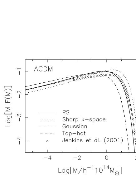
Figure 13: Differential multiplicity functions $F(M)$ with the effect of the spatial correlation in a $\Lambda$CDM model. The solid, the dotted, the dashed and the dash-dotted lines denote $F(M)$ for the PS, the sharp $k$-space, the Gaussian and the top-hat filters. The crosses indicate the mass function given by Jenkins et al. (2001), which was obtained by fitting their $N$-body simulation.

6 Discussion

In this section we discuss some uncertainties in calculation of the mass function.

6.1 Mass-smoothing scale relation

So far we use a simple mass-smoothing scale relation, $M=4\pi R^{3}\bar{\rho}/3$ and $k_{c}R=\pi$ in the case of scale-free power spectra. By changing this relation, the mass function may be affected as follows. It should be noted that we calculate the mass function against the normalized mass $M/M_{*}$ and $M_{*}$ is defined so as to $\sigma_{0}(M_{*})=1$ with scale-free power spectra. Thus the mass function does not scale in mass by changing the relation, even in the case of the Gaussian filter. This effect appears via the spatial correlation in the case of the sharp $k$-space filter.

The ratio of the cut-off wave number for the simple relation ($k_{c}$) to that given by the LC method ($k_{c,\rm LC}$), $k_{c}/k_{c,\rm LC}=(2\pi^{2}/9)^{1/3}\sim 1.3$. Thus the effect of the spatial correlation is weakened because the correlation at distance $r$ is described by the combination of $k_{c}r$, and the probability $P(M_{1}|M_{2})$ is obtained by integrating $P(r,M_{1}|M_{2})$ from 0 to $R$ respect to $r$. We checked this uncertainty, but the effect does not change our results qualitatively, especially at larger mass scale ($M\gtrsim M_{*}$).

If we use a realistic power spectrum, for example CDM models, the normalization of the mass spectrum $\sigma_{0}(M)$ becomes not arbitrary. In observation the normalization of the power spectrum is given by the amplitude at $8h^{-1}$Mpc with the top-hat filter with the bias parameter. This leads that the amplitude at that scale does not become unity in cases of other filters. In Fig.5.4, we adopt the LC method as a usual manner. We have found that when we use the simple relation the differences between the PS and the mass functions with the Gaussian and the sharp $k$-space filters becomes large compared with those in the case of the LC method. Part of the remaining differences is owing to the difference of the amplitude of the power spectrum.

6.2 Effect of non-spherical collapse

Throughout this paper, we analyzed the mass function under the simplification of the spherical collapse, in which the critical density contrast for collapse is $\delta_{c}=1.69$. However, in more realistic condition, objects collapse nonspherically. Monaco (1995; 1997a, b; 1998) showed that the first collapse, which means one-dimensional or pancake collapse, occurs during more short time-scale. Fitting the PS mass function to the resultant mass function, he obtained an effective density contrast $\delta_{c}\simeq 1.5$. This predicts larger number density of halos at larger scale compared to the PS, such as the effect of the spatial correlation. Apparently this seems to enhance the difference of the mass function including the effects of the filtering, peak, and spatial correlation. It will be correct when we consider the subsequent evolution of baryonic component included in halos because shock heating of gas occurs at the first collapse. Even so, in analyses of the mass function by using $N$-body simulations which is in good agreement with the theoretical PS mass function, it is not trivial that the condition of the identification of isolated halos is corresponding to the first collapse. Actually such identified halos are rather spherical. This means that the effective critical density is larger than 1.5 and that the second or third collapse criterion will be better than the first collapse one. If so, the non-spherical effect will hardly affect our results, unless the mixture of the effects emerges as shown in Fig.5.3.

7 Summary and Conclusions

In this paper, we analyzed the following three effects on the mass function: the filtering effect of the density fluctuation field, the peak ansatz in which objects collapse around density maxima, and the spatial correlation of density contrasts within a region of a collapsing halo because objects have non-zero finite volume. It has been shown by many authors that the PS mass function agrees with $N$-body results well. However it had been also unclear why the PS mass function works well. Taking into account the above three effects and using an integral formulation proposed by Jedamzik (1995), we tried to solve the missing link in the PS formalism. While YNG showed that the effect of the spatial correlation alters the original PS mass function, in this paper, we showed that the filtering effect almost cancels out the effect of the spatial correlation and that the original PS is almost recovered by combining these two effects, particularly in the case of the top-hat filter. As we shown in Fig.5.4, the mass function with this filter is in good agreement with that given by a $N$-body simulation (Jenkins et al. 2001). On the other hand, as for the peak effect, the resultant mass functions are changed dramatically and not in agreement especially at low-mass tails in the cases of the Gaussian and the sharp $k$-space filters.

In the sharp $k$-space filters, as shown by PH90 and BCEK, a density contrast at a point changes as the smoothing scale decreases because a new Fourier mode with an uncorrelated phase with other modes gives the density contrast an additional value such as Markovian random walk, which originates the so-called fudge-factor-of-two. On the other hand, when using general filters, we cannot expect that the trajectory of density contrast against the smoothing scale behaves like Markovian random walk. Then the factor of two is lost. We confirmed the result by PH90 and BCEK by using the other formalism proposed by Jedamzik (1995), against the filtering effect which we referred in this paper. The number density of halos decreases at larger mass scale compared to a typical mass scale which gives unity variance, and increase at smaller mass scale. Besides we found that the slope at smaller scale does not change. Thus apparently the shape of the multiplicity function $F(M)$ scales horizontally against the mass scale. This effect can be interpreted as the correlation of the Fourier modes, $\delta_{\bf k}$, in a statistical sense.

We also investigated the effect of the peak ansatz in which objects collapse around density maxima and which is often considered in structure formation theories. In the case of the Gaussian filter, this makes the low-mass tail of the multiplicity function shallower than the PS dramatically. We found that this difference can be interpreted by the behavior of the probability $P(M_{1}|M_{2})$ near $M_{1}\sim M_{2}$. $P(M_{1}|M_{2})$ increases above a half at that scale while it remains a half in the sharp $k$-space filter. On the other hand, in the case of the top-hat filter, we cannot deal with this effect correctly because this filter does not smooth out the density field adequately so as to be able to differentiate the density contrasts respect to the spatial coordinate due to the sharpness on the edge of the filter. While this trouble may be removed to adopt another filter with a rounded edge, it will originate complicated mathematical difficulty.

The effect of the spatial correlation only in the case of the sharp $k$-space filter was already considered in YNG. They showed that, in contrast to the filtering effect shown here, the mass function predicts more number of halos at larger mass scale, $M\gtrsim M_{*}$, and less number at smaller scale, $M\lesssim M_{*}$. This is apparently corresponding to scaling the mass scale to larger one. This property is caused by decreasing correlation between density contrasts with different smoothing scales. By considering the other filters, we showed that such properties are weakened and the resultant mass functions become close to the original PS because the filtering effect strengths the mode correlation as mentioned above. We also showed, however, that the spatial correlation cannot correct the change of the slope of the low-mass tail in the case of the Gaussian filter which is caused by the peak effect and besides steepens the tail in the case of the sharp $k$-space filter. This is because the probability $P(M_{1}|M_{2})$ is mainly affected at $M_{1}\sim M_{2}$ almost independent of the absolute values of $M_{1}$ and $M_{2}$ by the peak effect, while mainly affected at $M_{1}\gtrsim M_{*}$ by the filtering effect and the spatial correlation. Probably we can confirm which filter is better by using a high resolution $N$-body simulation, while it may be difficult to obtain an adequate dynamic mass range to much smaller scale than $M_{*}$.

As a conclusion, the discrepancy with the PS shown by YNG, in which only the sharp $k$-space filter was considered, is almost canceled out by the filtering effect. The peak ansatz, which does not affect the mass function in the case of the top-hat filter due to the mathematical reason, causes a new discrepancy at low mass scale in the cases of the Gaussian and the sharp $k$-space filters. A new filter similar to the top-hat filter but differentiable will be required in order to consider more realistic situation of collapsing halos.

It should be noted that the discrepancy is not perfectly canceled by the filtering effect and the spatial correlation, especially at larger mass scale, $M\gtrsim M_{*}$. This scale is corresponding to the galaxy clusters. Several authors have tried to determine the cosmological parameters and the normalization factor of the power spectrum by comparing the PS mass function to the observational cluster abundance (e.g., Bahcall 2000). We should pay attention to the fact that the results by such approach may depend on the model mass function.

We discussed an important effect of the non-spherical collapse, which has been investigated by Monaco (1995; 1997a, b; 1998). He found that if we adopt the first shell crossing as the collapse criterion, the resultant mass function predicts larger number density of halos at larger scale $M\gtrsim M_{*}$ and smaller number density at smaller scale $M\lesssim M_{*}$ compared to the PS because the time-scale of collapse decreases. This effect will enhance the difference between the PS and the mass function given by a full statistics with the effects taken into account in this paper and with the non-spherical collapse. Thus when we consider the evolution of the baryonic component, we should pay attention this effect. However, the agreement of the PS with the mass function given by many $N$-body simulations will be obtained by adopting the second or the third shell crossing as the collapse because identified objects as halos are rather spherical, not sheet-like or filamentary.

We found that the effects we considered becomes more prominent in larger spectral index $n$. In CDM model, the effective spectral index $n$ is less than -2 at galactic scale. Therefore in a realistic power spectrum the difference of the low-mass tail of the mass function from the PS may be negligible. However, at larger scale $M\gtrsim M_{*}$, the difference remains. This may leads a systematic error when the cosmological parameters are estimated by comparing observations such as cluster abundance with the PS. Thus we need more detailed study on the mass function.

Finally we should note that the approximation method used here is different from the excursion set approach. In the calculation of $P(M_{1}|M_{2})$, we considered only two different mass scales, $M_{1}$ and $M_{2}$. However, more strictly speaking, the probability must be subject to an additional condition, that is, the object with $M_{2}$ is an isolated object. In other words, the collapsing condition of objects $M_{2}$ must describe the first upcrossing above $\delta_{c}$. This is essentially the same as the cloud-in-cloud problem and the overlapping problem which was pointed out by YNG. Even so, we believe that the approximation used here is adequate to resolve the mystery in the PS formalism because the fact that the filtering effect correlates different Fourier modes leads to enhance the probability that the objects $M_{2}$ in our formulation are isolated. This conjecture can be stressed by the similarity of the mass functions shown here and the Monte Carlo approach to solve the excursion set formalism with the general filters, as mentioned above. In future, this will be proved by using a high resolution $N$-body simulation numerical experimentally.

Appendix A Formulation of $P(M_{1}|M_{2})$ for general filters

In this paper, we only considered Gaussian random fields. It is well-known that the Gaussian field is perfectly determined by the two-point correlation function. In the followings, we show the form of the probability required to analyze the mass function firstly, and show the correlation and the auto-correlation functions, which are introduced as covariances in multi-variate Gaussian distribution functions, in the case of the power-law power spectrum, $P(k)\equiv\langle|\delta_{\bf k}|^{2}\rangle=Ak^{n}$, where $A$ is the amplitude, which is normalized so as to be unity at $M=M_{*}$, and the angle brackets stand for the ensemble average.

The kernel in eq.(14), $P(M_{1}|M_{2})$, is generally expressed as a conditional probability. Since we need at least two Gaussian fields with smoothing scale $M_{1}$ and $M_{2}$ $(M_{1}\leq M_{2})$, or $R_{1}$ and $R_{2}$ $(R_{1}\leq R_{2})$ in terms of length as mentioned in §2, multi-variate Gaussian distribution functions are required. Here we define ${\bf V}^{N}\equiv(x_{1},\cdots,x_{N})$ as a vector of $N$ Gaussian distributed variables and ${\bf C}^{N}$ as a condition for $N$ variables. The distribution function for a variable $x_{N}$ under the condition ${\bf C}^{N-1}$ is written by Bayes’ theorem,

$$p(x_{N}|{\bf C}^{N-1})dx_{N}=\frac{p(x_{N},{\bf C}^{N-1})dx_{N}}{p({\bf C}^{N-1})},$$ (A1)

where $p({\bf V})$ is a multi-variate Gaussian distribution function. In this paper, the condition ${\bf C}^{N}$ means a criterion of collapse for larger objects, $M_{2}$. When we do not consider the peak condition, the vector ${\bf V}$ is two-variable one, ${\bf V}^{2}=(\delta_{2},\delta_{1})$ and the condition ${\bf C}$ constrains one variable $\delta_{2}$, ${\bf C}^{1}=(\delta_{2}=\delta_{2c})$. Note that the points for $\delta_{1}$ and $\delta_{2}$ are generally not the same if the spatial correlation is taken into account. When we consider the peak condition, eleven-variate Gaussian distribution is required as ${\bf V}^{11}=(\delta_{2},\eta_{i},\zeta_{ij},\delta_{1})$, where $i=1,2,3$ and $i\leq j$. Note that $\eta_{i}$ and $\zeta_{ij}$ are derivatives of $\delta_{2}$ respect to the coordinate $x_{i}$. Conditions for $\eta_{i}$ and $\zeta_{ij}$ are determined such that the density has a local maximum at the point $M_{2}$.

By using a covariance matrix ${\bf M}$, the $N$-variate Guassian distribution function is generally written as

$$p({\bf V}^{N})d{\bf V}^{N}=\frac{\exp[-Q/2]}{\sqrt{(2\pi)^{N}\det({\bf M})}}d{\bf V}^{N},$$ (A2)

where

$$Q = {\bf V}{\bf M}^{-1}{\bf V}^{\rm T}$$ (A3)

$$M_{ij} = \langle(x_{i}-\langle x_{i}\rangle)(x_{j}-\langle x_{j}\rangle)\rangle.$$ (A4)

This shows that the multi-variate Gaussian distribution is perfectly determined by correlations for any two variables. Thus what we do is to calculate the covariance matrix ${\bf M}$ for given variables.

As shown in YNG, the following covariances have non-zero values:

$$\langle\delta_{1}^{2}\rangle = \sigma_{r}^{2},\qquad\langle\delta_{2}^{2}\rangle=\sigma_{0}^{2},\qquad\langle\delta_{1}\delta_{2}\rangle=\xi_{0},\qquad\langle\eta_{i}\eta_{j}\rangle=\frac{\sigma_{1}^{2}}{3}\delta_{ij},$$

$$\langle\zeta_{ij}\zeta_{kl}\rangle = \frac{\sigma_{2}^{2}}{15}(\delta_{ij}\delta_{kl}+\delta_{ik}\delta_{jl}+\delta_{il}\delta_{jk}),\qquad\langle\delta_{2}\zeta_{ij}\rangle=-\frac{\sigma_{1}^{2}}{3}\delta_{ij},\qquad\langle\delta_{1}\zeta_{ij}\rangle=-\frac{\xi_{1}}{3}\delta_{ij},$$ (A5)

where $\delta_{ij}$ is the Kronecker’s delta. Variances and correlations $\sigma_{r},\sigma_{i}$, and $\xi_{i}$ are defined as

$$\xi_{l}(r) = \frac{4\pi}{(2\pi)^{3}}\int_{0}^{\infty}{\tilde{W}}(kR_{1}){\tilde{W}}(kR_{2})P(k)\frac{\sin kr}{kr}k^{2l+2}dk=\frac{4\pi A}{(2\pi)^{3}}\frac{1}{R_{2}^{n+2l+3}}I_{n+2l+2}(r),$$ (A6)

$$\sigma_{l}^{2} = \frac{4\pi}{(2\pi)^{3}}\int_{0}^{\infty}{\tilde{W}}^{2}(kR_{2})P(k)k^{2l+2}dk=\frac{4\pi A}{(2\pi)^{3}}\frac{1}{R_{2}^{n+2l+3}}I_{n+2l+2},$$ (A7)

$$\sigma_{r}^{2} = \frac{4\pi}{(2\pi)^{3}}\int_{0}^{\infty}{\tilde{W}}^{2}(kR_{1})P(k)k^{2}dk=\frac{4\pi A}{(2\pi)^{3}}\frac{1}{R_{1}^{n+3}}I_{n+2}.$$ (A8)

Clearly $\xi_{l}(r)$ means the $2l$-th moment of the two-point correlation function, $\sigma_{l}^{2}$ is the $2l$-th moment of the variance with the smoothing scale $R_{2}$, and $\sigma_{r}^{2}$ is the variance with the scale $R_{1}$. The subscript $r$ stands for the value with the scale $R_{1}$ because generally it is separated by $r$ from the center of the object with the scale $R_{2}$ in this paper. It should be noted that $\xi_{l}(r)\to\sigma_{l}^{2}$ for $r\to 0$ and $R_{1}\to R_{2}$. The integrals $I_{m}(r)$ and $I_{m}$ are calculated for specific window function ${\tilde{W}}(kR)$ in the next section.

In the followings, the peak condition is taken into account. In the case without the condition, the probabilities are obtained by neglecting quantities concerning $\eta_{i}$ and $\zeta_{ij}$. Here we diagonalize the Hesse matrix $\zeta_{ij}$ by introducing the eigenvalues $(-\lambda_{1},-\lambda_{2},-\lambda_{3})$ with the order $\lambda_{1}\geq\lambda_{2}\geq\lambda_{3}$, and the Euler angles $\alpha^{\prime},\beta^{\prime}$ and $\gamma^{\prime}$. The volume element concerning the Hesse matrix becomes

$$\prod_{\stackrel{{\scriptstyle\scriptstyle i,j=1,2,3}}{{i\leq j}}}d\zeta_{ij}=|(\lambda_{1}-\lambda_{2})(\lambda_{2}-\lambda_{3})(\lambda_{3}-\lambda_{1})|d\lambda_{1}d\lambda_{2}d\lambda_{3}\sin\beta^{\prime}d\beta^{\prime}d\alpha^{\prime}d\gamma^{\prime}.$$ (A9)

Here we normalize the variables,

$$\nu_{1}\equiv\frac{\delta_{1}}{\sigma_{r}},\nu_{2}\equiv\frac{\delta_{2}}{\sigma_{0}},x^{\prime}\equiv\frac{\lambda_{1}+\lambda_{2}+\lambda_{3}}{\sigma_{2}},y^{\prime}\equiv\frac{\lambda_{1}-\lambda_{3}}{2\sigma_{2}},z^{\prime}\equiv\frac{\lambda_{1}-2\lambda_{2}+\lambda_{3}}{2\sigma_{2}}.$$ (A10)

The peak condition constrains the derivatives of $\delta$ to be $\mbox{$\eta$}=0$ and each diagonal component $-\lambda_{i}$ is less than 0, which means $-y^{\prime}\leq z^{\prime}\leq y^{\prime}$ and $y^{\prime}\leq 0$. The covariances are transformed as

$$\langle\nu_{1}^{2}\rangle=1,\langle\nu_{2}^{2}\rangle=1,\langle x^{\prime}\nu_{2}\rangle=\gamma,\langle\nu_{1}\nu_{2}\rangle=\epsilon(r),\langle x^{\prime}\nu_{1}\rangle=\mu(r),\langle x^{\prime 2}\rangle=1,\langle y^{\prime 2}\rangle=\frac{1}{15},\langle z^{\prime 2}\rangle=\frac{1}{5},$$ (A11)

where $\epsilon(r)$, $\mu(r)$ and $\gamma$ are written as

$$\epsilon(r) = \langle\nu_{1}\nu_{2}\rangle=\frac{\xi_{0}(r)}{\sigma_{r}\sigma_{0}},$$ (A12)

$$\mu(r) = \langle x^{\prime}\nu_{1}\rangle=\frac{\xi_{1}(r)}{\sigma_{r}\sigma_{2}},$$ (A13)

$$\gamma = \langle x^{\prime}\nu_{2}\rangle=\frac{\sigma_{1}^{2}}{\sigma_{0}\sigma_{2}},$$ (A14)

and $\mu(r)\to\gamma$ for $r\to 0$ and $R_{1}\to R_{2}$. In order to obtain the exponents of probabilities, we define the following variables:

$$Q_{a} = \frac{1-\gamma^{2}}{1-\epsilon^{2}-\mu^{2}-\gamma^{2}+2\epsilon\mu\gamma}\left(\nu_{1}+\frac{\mu\gamma-\epsilon}{1-\gamma^{2}}\nu_{2}+\frac{\epsilon\gamma-\mu}{1-\gamma^{2}}x^{\prime}\right)^{2},$$ (A15)

$$Q_{b} = \frac{(x^{\prime}-\gamma\nu_{2})^{2}}{1-\gamma^{2}},$$ (A16)

$$Q_{c} = \nu_{2}^{2}+15y^{\prime 2}+5z^{\prime 2}+3\frac{|\mbox{$\eta$}|^{2}}{\sigma_{1}^{2}},$$ (A17)

where we omit the argument $r$ of $\epsilon(r)$ and $\mu(r)$ for simplicity. After integrating the volume element over the Euler angles, we obtain

$$p(\nu_{1},\nu_{2},\mbox{$\eta$},x^{\prime},y^{\prime},z^{\prime})d\nu_{1}d\nu_{2}d^{3}\mbox{$\eta$}dx^{\prime}dy^{\prime}dz^{\prime}$$ (A18)

$$= \frac{3(15)^{5/2}|y^{\prime}(y^{\prime 2}-z^{\prime 2})|}{8\sqrt{2}\pi^{7/2}\sigma_{1}^{3}\sqrt{1-\epsilon^{2}-\mu^{2}-\gamma^{2}+2\epsilon\mu\gamma}}\exp\left[-\frac{Q_{a}+Q_{b}+Q_{c}}{2}\right]d\nu_{1}d\nu_{2}d^{3}\mbox{$\eta$}dx^{\prime}dy^{\prime}dz^{\prime},$$

$$p(\nu_{2},\mbox{$\eta$},x^{\prime},y^{\prime},z^{\prime})d\nu_{2}d^{3}\mbox{$\eta$}dx^{\prime}dy^{\prime}dz^{\prime}$$ (A19)

$$= \frac{3(15)^{5/2}|y^{\prime}(y^{\prime 2}-z^{\prime 2})|}{8\pi^{3}\sigma_{1}^{3}\sqrt{1-\gamma^{2}}}\exp\left[-\frac{Q_{b}+Q_{c}}{2}\right]d\nu_{2}d^{3}\mbox{$\eta$}dx^{\prime}dy^{\prime}dz^{\prime}.$$

The latter equation is the same as eq.(A7) in BBKS. From the Bayes’ theorem, the required probability is written under the above condition against $\nu_{2},\mbox{$\eta$},x^{\prime},y^{\prime}$ and $z^{\prime}$ as

$$P(r,M_{1}|M_{2})=\sqrt{\frac{1-\gamma^{2}}{2\pi(1-\epsilon^{2}-\mu^{2}-\gamma^{2}+2\epsilon\mu\gamma)}}\frac{\int_{0}^{\infty}dx^{\prime}f(x^{\prime})\int_{\nu_{1c}}^{\infty}d\nu_{1}e^{-(Q_{a}+Q_{b})/2}}{\int_{0}^{\infty}dx^{\prime}f(x^{\prime})e^{-Q_{b}/2}},$$ (A20)

where

$$f(x^{\prime}) = \left(\int_{0}^{x^{\prime}/4}dy^{\prime}\int_{-y^{\prime}}^{y^{\prime}}dz^{\prime}+\int_{x^{\prime}/4}^{x^{\prime}/2}dy^{\prime}\int_{3y^{\prime}-x^{\prime}}^{y^{\prime}}dz^{\prime}\right)|y^{\prime}(y^{\prime 2}-z^{\prime 2})|\exp\left(-\frac{15}{2}y^{\prime 2}-\frac{5}{2}z^{\prime 2}\right)$$ (A21)

$$= \left(\int_{-x^{\prime}/4}^{0}dz^{\prime}\int_{-z^{\prime}}^{(z^{\prime}+x^{\prime})/3}dy^{\prime}+\int_{0}^{x^{\prime}/2}dz^{\prime}\int_{z^{\prime}}^{(z^{\prime}+x^{\prime})/3}dy^{\prime}\right)[y^{\prime}(y^{\prime 2}-z^{\prime 2})]\exp\left(-\frac{15}{2}y^{\prime 2}-\frac{5}{2}z^{\prime 2}\right)$$

$$= \frac{1}{2250}\left[-15x^{\prime}\exp\left(-\frac{5}{8}x^{\prime 2}\right)+\sqrt{10\pi}\left\{{\rm erf}\left(\frac{x^{\prime}}{2}\sqrt{\frac{5}{2}}\right)+{\rm erf}\left(x^{\prime}\sqrt{\frac{5}{2}}\right)\right\}\right],$$

with the definition of the error function,

$${\rm erf}(x)=\frac{2}{\sqrt{\pi}}\int_{0}^{x}e^{-t^{2}}dt.$$ (A22)

Note that the form of $f(x)$ is different from eq.(A15) in BBKS because they considered not the probability but the number density of peaks. Finally, if we take into account the spatial correlation, that is, the different points of $\delta_{1}$ and $\delta_{2}$, we need to spatially average the above probability over the region $R_{2}$ in order to obtain $P(M_{1}|M_{2})$,

$$P(M_{1}|M_{2})=\frac{\int_{0}^{R}P(r,M_{1}|M_{2})4\pi r^{2}dr}{\int_{0}^{R}4\pi r^{2}dr}.$$ (A23)

Appendix B Correlation coefficients for specific filters

In the followings, we give the specific forms of the correlation coefficients $\epsilon(r),\mu(r)$ and $\gamma$ for the three filters, the top-hat, the Gaussian, and the sharp $k$-space filters, and for the spectral index $n=0$ and $-2$, which are important values when considering formation process of galaxies and galaxy clusters in a CDM universe.

Here, for convenience, we define the following dimensionless variables,

$$y=kR_{2},\quad z=R_{1}/R_{2},\quad s=r/R_{2}.$$ (B1)

By using these variables, the correlation coefficients are written as follows:

$$\gamma=\frac{I_{n+4}}{\sqrt{I_{n+2}I_{n+6}}},\qquad\epsilon(r)=z^{\frac{n+3}{2}}\frac{I_{n+2}(r)}{I_{n+2}},\qquad\mu(r)=z^{\frac{n+3}{2}}\frac{I_{n+4}(r)}{\sqrt{I_{n+2}I_{n+6}}}.$$ (B2)

Thus, the problem is reduced to calculating the integrals $I_{m}(r)$ and $I_{m}$.

B.1 Top-hat filter

In the case of the top-hat filter, the behavior of the correlations changes at the boundary of an object with the smoothing scale $R_{2}$. So we define the regions I, II, and III as

1. Internal: $r\leq R_{2}-R_{1}$,

2. Crossing: $R_{2}-R_{1}\leq r\leq R_{2}+R_{1}$,

3. External: $R_{2}+R_{1}\leq r$,

and the following new variables as

$$a=1-z-s,\quad b=1-z+s,\quad c=1+z-s,\quad d=1+z+s.$$ (B3)

Actually the region III is not considered in our analyses, but we express the explicit forms of the correlations for the region III in the following.

The generic forms of the integrals can be expressed as

$$I_{m}(r) = \int_{0}^{\infty}\frac{9}{y^{6}z^{3}}(\sin yz-yz\cos yz)(\sin y-y\cos y)y^{m}\frac{\sin ys}{ys}dy,$$ (B4)

$$I_{m} = \int_{0}^{\infty}\frac{9}{y^{6}}(\sin y-y\cos y)^{2}y^{m}dy.$$ (B5)

The solutions for $m=0,2,4$ and 6 depend on the region I, II and III as follows:

$$I_{0}(r)=\frac{\pi}{640sz^{3}}[ - 6|a|(1-z)a^{4}+\mbox{sign}(a)(a^{6}-30za^{4})$$ (B6)

$$+ 6|b|(1-z)b^{4}+\mbox{sign}(b)(-b^{6}+30zb^{4})$$

$$+ 6|c|(1+z)c^{4}+\mbox{sign}(c)(-c^{6}-30zc^{4})$$

$$- 6|d|(1+z)d^{4}+\mbox{sign}(d)(d^{6}+30zd^{4})],$$

$$I_{2}(r)=\frac{9\pi}{192sz^{3}}[ 4|a|(1-z)a^{2}+\mbox{sign}(a)(-a^{4}+12za^{2})$$ (B7)

$$- 4|b|(1-z)b^{2}+\mbox{sign}(b)(b^{4}-12zb^{2})$$

$$- 4|c|(1+z)c^{2}+\mbox{sign}(c)(c^{4}+12zc^{2})$$

$$+ 4|d|(1+z)d^{2}+\mbox{sign}(d)(-d^{4}-12zd^{2})],$$

$$I_{4}(r)=\frac{9\pi}{16sz^{3}}[ - 2|a|(1-z)+\mbox{sign}(a)(a^{2}-2z)$$ (B8)

$$+ 2|b|(1-z)+\mbox{sign}(b)(-b^{2}+2z)$$

$$+ 2|c|(1+z)+\mbox{sign}(c)(-c^{2}-2z)$$

$$- 2|d|(1+z)+\mbox{sign}(d)(d^{2}+2z)],$$

$$I_{6}(r)=\frac{9\pi}{8sz^{3}}[-\mbox{sign}(a)+\mbox{sign}(b)+\mbox{sign}(c)-\mbox{sign}(d)],$$ (B9)

or more explicitly,

$$I_{0}(r) = \left\{\begin{array}[]{ll}\displaystyle{\frac{\pi}{20}(-3z^{2}+15-5s^{2})}&\qquad\mbox{I}\\ \displaystyle{\frac{\pi}{640sz^{3}}[10(z^{6}-9z^{4}+16z^{3}-9z^{2}+1)+48s(-z^{5}+5z^{3}+5z^{2}-1)}&\\ \displaystyle{\quad+90s^{2}(z^{4}-2z^{2}+1)+80s^{3}(-z^{3}-1)+30s^{4}(z^{4}+1)-2s^{6}]}&\qquad\mbox{II}\\ \displaystyle{\frac{\pi}{2s}}&\qquad\mbox{III},\end{array}\right.$$ (B14)

$$I_{2}(r) = \left\{\begin{array}[]{ll}\displaystyle{\frac{3\pi}{2}}&\qquad\mbox{I}\\ \displaystyle{\frac{3\pi}{32sz^{3}}[-3(1-z^{2})^{2}+8s(1+z^{3})-6s^{2}(1+z^{2})+s^{4}]}&\qquad\mbox{II}\\ \displaystyle{0}&\qquad\mbox{III},\end{array}\right.$$ (B18)

$$I_{4}(r) = \left\{\begin{array}[]{ll}\displaystyle{0}&\qquad\mbox{I}\\ \displaystyle{\frac{9\pi}{8sz^{3}}(z^{2}-s^{2}+1)}&\qquad\mbox{II}\\ \displaystyle{0}&\qquad\mbox{III},\end{array}\right.$$ (B22)

$$I_{6}(r) = \left\{\begin{array}[]{ll}\displaystyle{0}&\qquad\mbox{I}\\ \displaystyle{\frac{9\pi}{4sz^{3}}}&\qquad\mbox{II}\\ \displaystyle{0}&\qquad\mbox{III},\end{array}\right.$$ (B26)

and

$$I_{0} = \frac{3\pi}{5},$$ (B27)

$$I_{2} = \frac{3\pi}{2},$$ (B28)

$$I_{4} = \lim_{y\to\infty}\frac{9}{4y}[-2+2y^{2}+2\cos{2y}+y\sin{2y}]\to\infty,$$ (B29)

$$I_{6} = \lim_{y\to\infty}\frac{9}{24}[12y+4y^{3}+18y\cos{2y}-15\sin{2y}+6y^{2}\sin{2y}]\to\infty.$$ (B30)

The correlation coefficients are obtained by using the above integrals for the spectral index $n=0$,

$$\gamma = 0,$$ (B31)

$$\epsilon(r) = z^{3/2}\frac{I_{2}(r)}{3\pi/2}=\left\{\begin{array}[]{ll}\displaystyle{z^{3/2}}&\qquad\mbox{I}\\ \displaystyle{\frac{z^{-3/2}}{16s}(-3(1-z^{2})^{2}+8s(1+z^{3})-6s^{2}(1+z^{2})+s^{4})}&\qquad\mbox{II}\\ \displaystyle{0}&\qquad\mbox{III},\end{array}\right.$$ (B35)

$$\mu(r) = z^{3/2}\frac{I_{4}(r)}{\sqrt{I_{2}I_{6}}}\to 0,$$ (B36)

and for $n=-2$,

$$\gamma = 0,$$ (B37)

$$\epsilon(r) = z^{1/2}\frac{I_{0}(r)}{3\pi/5}=\left\{\begin{array}[]{ll}\displaystyle{\frac{z^{1/2}}{12}(-3z^{2}+15-5s^{2})}&\qquad\mbox{I}\\ \displaystyle{\frac{z^{-5/2}}{384s}[10(z^{6}-9z^{4}+16z^{3}-9z^{2}+1)+48s(-z^{5}+5z^{3}+5z^{2}-1)}\\ \qquad\displaystyle{+90s^{2}(z^{4}-2z^{2}+1)-80s^{3}(z^{3}+1)+30s^{4}(z^{2}+1)-2s^{6}]}&\qquad\mbox{II}\\ \displaystyle{\frac{5z^{1/2}}{6s}}&\qquad\mbox{III},\end{array}\right.$$ (B42)

$$\mu(r) = z^{1/2}\frac{I_{2}(r)}{\sqrt{I_{0}I_{4}}}\to 0.$$ (B43)

These show that we cannot deal with the configuration of density peaks, at least statistically, in the case of the top-hat filter because of the divergence of $I_{4}$ and $I_{6}$ to infinity. This may be originated by the sharpness of the window function, which do not adequately smooth out density fields so as to be differentiable.

Here we show that the peak condition is canceled out in the calculation of the probability $P(r,M_{1}|M_{2})$. Now $\mu(r)=\gamma=0$, then the eq.(A20) becomes

$$P(r,M_{1}|M_{2})=\sqrt{\frac{1}{2\pi(1-\epsilon^{2})}}\frac{\int_{0}^{\infty}dx^{\prime}f(x^{\prime})\int_{\nu_{1c}}^{\infty}d\nu_{1}e^{-\frac{Q_{a}+Q_{b}}{2}}}{\int_{0}^{\infty}dx^{\prime}f(x^{\prime})e^{-\frac{Q_{b}}{2}}},$$ (B44)

and the exponents become

$$Q_{a}=\frac{(\nu_{1}-\epsilon\nu_{2c})^{2}}{1-\epsilon^{2}},\qquad Q_{b}=x^{\prime 2}.$$ (B45)

Because the exponent $Q_{a}$ does not depend on $x^{\prime}$, we can cancel the integration respect to $x^{\prime}$ as follows,

$$P(r,M_{1}|M_{2})=\frac{1}{\sqrt{2\pi(1-\epsilon^{2})}}\int_{\nu_{1c}}^{\infty}d\nu_{1}e^{-\frac{Q_{a}}{2}}.$$ (B46)

This is the same form as the probability not taking into account the peak effect.

B.2 Gaussian filter

The generic forms of the integrals are expressed by using the confluent hypergeometric function and the gamma function as follows:

$$I_{m}(r) = \int_{0}^{\infty}e^{-\frac{y^{2}}{2}(1+z^{2})}y^{m}\frac{\sin ys}{ys}dy=\frac{\Gamma(\frac{1+m}{2})}{[2(1+z^{2})]^{\frac{1+m}{2}}}{}_{1}F_{1}\left(\frac{1+m}{2};\frac{3}{2};-\frac{s^{2}}{2(1+z^{2})}\right),$$ (B47)

$$I_{m} = \int_{0}^{\infty}e^{-y^{2}}y^{m}dy.$$ (B48)

Specifically,

$$I_{0}(r) = \frac{\pi}{2s}\mbox{erf}\left[\frac{s}{\sqrt{2(1+z^{2})}}\right],$$ (B49)

$$I_{2}(r) = \sqrt{\frac{\pi}{2}}\frac{1}{(1+z^{2})^{3/2}}e^{-\frac{s^{2}}{2(1+z^{2})}},$$ (B50)

$$I_{4}(r) = \sqrt{\frac{\pi}{2}}\frac{3}{(1+z^{2})^{5/2}}\left[1-\frac{s^{2}}{3(1+z^{2})}\right]e^{-\frac{s^{2}}{2(1+z^{2})}},$$ (B51)

$$I_{6}(r) = \sqrt{\frac{\pi}{2}}\frac{15}{(1+z^{2})^{7/2}}\left[1-\frac{2s^{2}}{3(1+z^{2})}+\frac{s^{4}}{15(1+z^{2})^{2}}\right]e^{-\frac{s^{2}}{2(1+z^{2})}},$$ (B52)

and

$$I_{m}=\frac{\Gamma(\frac{1+m}{2})}{2},\quad I_{0}=\frac{\sqrt{\pi}}{2},\quad I_{2}=\frac{\sqrt{\pi}}{4},\quad I_{4}=\frac{3\sqrt{\pi}}{8},\quad I_{6}=\frac{15\sqrt{\pi}}{16}.$$ (B53)

The correlation coefficients for $n=0$ are

$$\gamma = \sqrt{\frac{3}{5}},$$ (B54)

$$\epsilon(r) = \left(\frac{2z}{1+z^{2}}\right)^{3/2}e^{-\frac{s^{2}}{2(1+z^{2})}},$$ (B55)

$$\mu(r) = 4\sqrt{\frac{6}{5}}\frac{z^{3/2}}{(1+z^{2})^{5/2}}\left[1-\frac{s^{2}}{3(1+z^{2})}\right]e^{-\frac{s^{2}}{2(1+z^{2})}},$$ (B56)

and for $n=-2$,

$$\gamma = \frac{1}{\sqrt{3}},$$ (B57)

$$\epsilon(r) = \frac{\sqrt{\pi z}}{s}{\rm erf}\left[\frac{s}{\sqrt{2(1+z^{2})}}\right],$$ (B58)

$$\mu(r) = \sqrt{\frac{8}{3}}\frac{z^{1/2}}{(1+z^{2})^{3/2}}e^{-\frac{s^{2}}{2(1+z^{2})}}.$$ (B59)

B.3 Sharp $k$-space filter

Here we show the integrals by using the generic cut-off wavenumber $k_{c}$ which is introduced in the filter, $y_{c}=k_{c}R$. In this paper we showed the results for $y_{c}=\pi$. If the definition by the LC method is used, $y_{c}=(9\pi/2)^{1/3}$. The generic forms of the integrals are

$$I_{m}(r) = \int_{0}^{y_{c}}y^{m}\frac{\sin{ys}}{ys}dy=\frac{y_{c}^{1+m}}{1+m}{}_{1}F_{2}\left[\frac{1+m}{2};\frac{3}{2},\frac{3+m}{2};-\frac{(sy_{c})^{2}}{4}\right],$$ (B60)

$$I_{m} = y_{c}^{m+1},$$ (B61)

where ${}_{1}F_{2}(a;b,c;z)$ is the generalized hypergeometric function. The specific forms of $I_{m}(r)$ are

$$I_{0}(r) = \frac{1}{s}\int_{0}^{sy_{c}}\frac{\sin{t}}{t}dt,$$ (B62)

$$I_{2}(r) = \frac{1}{s^{3}}[\sin{sy_{c}}-sy_{c}\cos{sy_{c}}],$$ (B63)

$$I_{4}(r) = \frac{1}{s^{5}}[sy_{c}(6-s^{2}y_{c}^{2})\cos{sy_{c}}-3(2-s^{2}y_{c}^{2})\sin{sy_{c}}],$$ (B64)

$$I_{6}(r) = \frac{1}{s^{7}}[-sy_{c}(120-20s^{2}y_{c}^{2}+s^{4}y_{c}^{4})\cos{sy_{c}}+5(24-12s^{2}y_{c}^{2}+s^{4}y_{c}^{4})\sin{sy_{c}}].$$ (B65)

The correlation coefficients for $n=0$ are

$$\gamma = \frac{\sqrt{21}}{5},$$ (B66)

$$\epsilon(r) = \frac{3z^{3/2}}{s^{3}y_{c}^{3}}[\sin{sy_{c}}-sy_{c}\cos{sy_{c}}],$$ (B67)

$$\mu(r) = \frac{\sqrt{21}z^{3/2}}{s^{5}y_{c}^{5}}[sy_{c}(6-s^{2}y_{c}^{2})\cos{sy_{c}}-3(2-s^{2}y_{c}^{2})\sin{sy_{c}}],$$ (B68)

and for $n=-2$,

$$\gamma = \frac{\sqrt{5}}{3},$$ (B69)

$$\epsilon(r) = \frac{z^{1/2}}{sy_{c}}\int_{0}^{sy_{c}}\frac{\sin{t}}{t}dt,$$ (B70)

$$\mu(r) = \frac{\sqrt{5}z^{1/2}}{s^{3}y_{c}^{3}}[\sin{sy_{c}}-sy_{c}\cos{sy_{c}}].$$ (B71)

References

• (1) Appel, A., & Jones, B.T. 1990, MNRAS, 245, 522
• (2) Bahcall, N.A. 2000, Phys.Β Rep., 333, 233
• (3) Bardeen, J.M., Bond, J.R., Kaiser, N., & Szalay, A.S. 1986, ApJ, 304, 15 (BBKS)
• (4) Bond, J.R., Cole, S., Efstathiou, G., & Kaiser, N. 1991, ApJ, 379, 440 (BCEK)
• (5) Bower, R. 1991, MNRAS, 248, 332
• (6) Doroshkevich, A.G. 1970, Astrofizika, 6, 581 (trans. Astrophysics, 6, 320 [1973])
• (7) Epstein, R.I. 1983, MNRAS, 205,207
• (8) Epstein, R.I. 1984, ApJ, 281, 545
• (9) Jedamzik, K. 1995, ApJ, 448, 1
• (10) Jenkins, A. et al. 2001, MNRAS, 321, 372
• (11) Gunn, J.E., & Gott, J.R. 1972, ApJ, 176, 1
• (12) Kauffmann, G., & White, S.D.M. 1993, MNRAS, 261, 921
• (13) Lacey, C.G., & Cole, S. 1993, MNRAS, 262, 627 (LC)
• (14) Manrique, A., & Salvador-SolΓ©, E. 1995, ApJ, 453, 6
• (15) Monaco, P. 1995, ApJ, 447, 23
• (16) Monaco, P. 1997a, MNRAS, 287, 753
• (17) Monaco, P. 1997b, MNRAS, 290, 439
• (18) Monaco, P. 1998, Fundam. Cosmic Phys., 19, 157
• (19) Nagashima, M., & Gouda, N. 1997, MNRAS, 287, 515
• (20) Peacock, J.A., & Heavens, A.F. 1985, MNRAS, 217, 805
• (21) Peacock, J.A., & Heavens, A.F. 1990, MNRAS, 243, 133 (PH90)
• (22) Press, W.H., & Schechter, P. 1974, ApJ, 187, 425 (PS)
• (23) Rodrigues, D.D.C., & Thomas, P.A. 1996, MNRAS, 282, 631
• (24) Sheth, R.K., & Tormen, G. 1999, MNRAS, 308, 119
• (25) Somerville, R.S., & Kolatt, T. 1998, MNRAS, 305, 1
• (26) Tomita, K. 1969, PTP, 42, 9
• (27) Yano, T., Nagashima, M., & Gouda, N. 1996, ApJ, 466, 1 (YNG)
• (28) Zel’dovich, Ya.B. 1970, Astrofizika, 6,319 (trans. Astrophysics, 6, 164 [1973])