Open and closed CDM isocurvature models contrasted with the CMB data

Abstract

We consider pure isocurvature cold dark matter models in the case of open and closed universes. We allow for a large spectral tilt and scan the 6-dimensional parameter space for the best fit to the COBE, Boomerang, and Maxima-1 data. Taking into account constraints from large-scale structure and big bang nucleosynthesis, we find a best fit with $\chi^{2}=121$, which is to be compared to $\chi^{2}=44$ of a flat adiabatic reference model. Hence the current data strongly disfavor pure isocurvature perturbations.

I Introduction

The recent measurements of the cosmic microwave background (CMB) temperature fluctuations by the Boomerang[4, 5] and Maxima-1[6, 7] balloon experiments and the DASI interferometer[8] have widely been regarded as indicating that we live in a $\Omega=1$ universe. This is so because the first acoustic peak is found at the multipole $\ell\simeq 200$, implying a flat universe. The firmness of such a conclusion is, however, based on certain tacit assumptions. In particular, when fitting the acoustic peak positions, one often assumes that the primordial perturbations are adiabatic and that the spectrum is nearly scale invariant.

If perturbations are adiabatic, the relative abundances of particle species are equal to their thermal equilibrium values. This is the case in the simplest, one-field inflation models but it is not a generic feature of inflation. More generally, perturbations can be either adiabatic or nonadiabatic; the latter would be perturbations in the particle number densities, or entropy perturbations, and are called isocurvature perturbations.

Because no generally accepted theory of inflation exists, it is natural to consider both adiabatic and isocurvature perturbations as being equally probable. This is the generic situation when more than one field is excited during inflation, such as is the case in double inflation [9] or in the minimally supersymmetric standard model with flat directions [10]. One should also note that in the pre-big-bang scenario, which has been proposed as an alternative to the inflationary universe, pre-big-bang axion field fluctuations give rise to an isocurvature perturbation spectrum [11]. Purely isocurvature $\Omega=1$ perturbations are, however, not consistent [12, 13, 14] with the observational data, but an admixture of (uncorrelated or correlated) adiabatic and isocurvature perturbations cannot be ruled out [14, 15, 16, 17]. However, if we do not insist on a flat universe, the situation could be different.

Recently, it was pointed out [18] that in the general (Gaussian) case the scalar power spectrum is a $5\times 5$ matrix $P_{ij}({\bf k})=\langle A_{i}({\bf k})A_{j}(-{\bf k})\rangle$, where $i,j$ label one adiabatic and four isocurvature modes [cold dark matter (CDM), baryon, neutrino density, and neutrino velocity] and their correlations. Here we shall focus on a purely isocurvature primordial perturbation in the CDM which has the power spectrum

$$P_{S}(k)=B\left(\sqrt{k^{2}-K}\right)^{n_{\rm iso}-4}~{},$$ (1)

where $n_{\rm iso}$ is the spectral index and $K=-H_{0}^{2}(1-\Omega)$ is the curvature. Since in curved space the Laplacian has eigenvalues $k^{2}-K$ instead of the $k^{2}$ of the flat case, the spectrum (1) is the simplest generalization of the flat space spectrum $k^{n_{\rm iso}-4}$.

In the flat, $\Omega=1$ case, definition (1) gives the power law $P_{S}(k)\propto k^{n_{\rm iso}-4}$, which is a natural form for the power spectrum, and approximates well the spectrum produced by typical inflation models with isocurvature perturbations in the region of interest. The scale-invariant spectrum has $n_{\rm iso}=1$. In principle, $n_{\rm iso}$ could well depend on $k$; here we shall assume that it is a constant (or varies very little) over the range of interest. In open and closed models the spatial curvature introduces a length scale and one expects this to be reflected in the form of the power spectrum. It is not obvious what would be the most natural modification to the power law for isocurvature models in curved space. This question has been studied only for specific models in the adiabatic case[19, 20]. Thus we stress that we are using a phenomenological power-law spectrum, which does not necessarily follow from any particular inflation model. We shall return to this point later in this paper.

After the clear detection of the acoustic peak around $\ell\simeq 200$ it became evident that the adiabatic models fit well to the data[4, 5, 7, 8, 21, 22]. However, this should not be taken as a proof that all pure isocurvature models are ruled out. Some unconventional combination of cosmological parameters, e.g., $\Omega\neq 1$ and a spectrum with a large tilt, could at least in principle give an equally good fit as do the adiabatic models.

Pure isocurvature models have two well-recognized problems: excess power at low multipoles and a peak structure that is roughly speaking out of phase by $\pi/2$ when compared to the adiabatic one [23]. Since the angular power in the low multipole region was measured quite firmly by the Cosmic Background Explorer (COBE), $\chi^{2}$ fitting forces the overall normalization constant in pure isocurvature models to be smaller than in the adiabatic case, which leads to too little power at higher multipoles. The easiest and perhaps the only way to compensate for this is to introduce a large spectral tilt. Moreover, since flat adiabatic models fit the observed peak at $\ell\simeq 200$ well, it is obvious that the $\ell\simeq 200$ peak falls between the first and second peaks of any flat isocurvature model. Accordingly, in our earlier study [14], the best-fit flat isocurvature model was found to have a large $\chi^{2}=116$ for 30 data points and 6 parameters whereas the best adiabatic model had $\chi^{2}=22$.

Thus we have two possibilities for a better isocurvature model. The first is to lower the total energy density parameter so much that the position of the first isocurvature peak fits to the observed peak at $\ell\simeq 200$, which means that we have to allow for an open universe ($\Omega<1$). The other possibility is to increase the total energy density parameter so much that the position of the second isocurvature peak fits the $\ell\simeq 200$ peak [24], implying a closed universe ($\Omega>1$). In this case the first isocurvature peak at $\ell\simeq 60\ldots 100$ should effectively disappear. In fact, a large spectral tilt would have precisely this effect since it would decrease the relative power at low $\ell$.

The purpose of the present paper is to study these possibilities systematically to find out if CDM isocurvature models are indeed completely ruled out by the presently available CMB data.

II Methods and results

In order to compare the isocurvature models with adiabatic ones we choose one representative well-fitted adiabatic model $(n_{\rm adi},\Omega_{m},\Omega_{\Lambda},\omega_{b},\omega_{c},\tau)=(0.98,0.38,0.62,0.021,0.13,0)$; cf. [4]. Using the same data sets and algorithm as for isocurvature models, we get $\chi^{2}=44$ for this adiabatic “reference” model. Fig. 3(b) confirms that this model fits well both the low $\ell$ part of the angular power spectrum and the acoustic peaks.

Our starting point for analyzing isocurvature models is a large grid with the following free parameters:

• $n_{\rm iso}=1.00\ldots 7.00$ (60 values)

• $\Omega_{m}=0.06\ldots 2.31$ (16 values)

• $\Omega_{\Lambda}=-1.00\ldots 1.10$ (14 values)

• $\omega_{b}=0.001\ldots 0.100$ (10 values)

• $\omega_{c}=0.01\ldots 1.60$ (15 values),

where $\Omega_{m}$ is the total matter density, $\Omega_{\Lambda}$ is the vacuum energy density, $\omega_{b}=h^{2}\Omega_{b}$ is the baryon density, and $\omega_{c}=h^{2}\Omega_{c}$ is the CDM density. The sixth free parameter is the overall normalization factor $B$ of Eq. (1). The Hubble constant $h$ is not a free parameter, since $h^{2}\Omega_{m}=\omega_{m}=\omega_{b}+\omega_{c}$. We use a top-hat prior $h=0.45\ldots 0.90$ and assume $\tau=0$ for the optical depth due to reionization. The angular power spectrum of all the models in the grid was calculated by CAMB [25] assuming isocurvature CDM initial conditions.

We use the $\chi^{2}$ method to compare models and data, because it allows us to quickly search a large parameter space. This method is approximate[20] and we do not attempt precise estimates for cosmological parameters or confidence levels. As will be seen, the conclusion is clear enough in ruling out the isocurvature models so that it is not necessary to go to a full maximum likelihood analysis[26].

Using the latest Boomerang data [4], together with Maxima-1 [6] and COBE data [27] we calculate $\chi^{2}$ for each model. The resulting best-$\chi^{2}$ contours in the $(\Omega_{m},\Omega_{\Lambda})$ plane are presented in Fig. 1 by gray levels. The best-fit model turns out to have $\chi^{2}=80$ with $(n_{\rm iso},\Omega_{m},\Omega_{\Lambda},\omega_{b},\omega_{c})=(2.00,2.11,-1.00,0.020,1.40)$. From Fig. 1(a) we see that the best-fit isocurvature models lie along two bands in the $(\Omega_{m},\Omega_{\Lambda})$ plane, the left band corresponding to open universes, and the right corresponding to closed universes. In the best-fit models the spectral index falls in the range $n_{\rm iso}=2\ldots 3$.

A detailed examination of the various pure isocurvature models allows us to conclude that the main problems are the spacings of the higher acoustic peaks and the slope in the (low $\ell$) Sachs–Wolfe region. COBE measured a close-to-flat $C_{\ell}$ spectrum, but the isocurvature models have a significant positive slope arising from the large primordial blue spectral tilt needed to get enough power at higher multipoles.

In the best-fit open models the prominent peak in the CMB data is fitted by the first acoustic peak of the isocurvature model. Fig. 1(a) shows that in the best-fit open region the first peak lies in the range $150\;\raise 1.29167pt\hbox{$<$\kern-7.5pt\raise-4.73611pt\hbox{$\sim$}}\;\ell\;\raise 1.29167pt\hbox{$<$\kern-7.5pt\raise-4.73611pt\hbox{$\sim$}}\;230$. Since the data do not show a high second peak, these models need a small baryon density $\omega_{b}$ to boost up the first peak and suppress the second peak. (In the adiabatic case, adding more baryons enhances odd acoustic peaks over even [23], but in the isocurvature case increasing $\omega_{b}$ boosts even peaks.) Actually, all the best-fit open models have a baryon density of $\omega_{b}=0.001$, which is the smallest value in the grid. However, even assuming such an unphysically low baryon density as $0.0005$ only gives about half of the power needed to fit the first peak, so not scanning below $\omega_{b}<0.001$ seems justified.

FIG. 1.: The best-$\chi^{2}$ contours on the $(\Omega_{m},\Omega_{\Lambda})$ plane. The best fit, which has $\chi^{2}=80$, is indicated by an asterisk ($\ast$) near to the lower right corner. The contours for deviation from the best fit are as follows: white $\Delta\chi^{2}<10$; light gray $10<\Delta\chi^{2}<40$; medium gray $40<\Delta\chi^{2}<100$; and dark gray $\Delta\chi^{2}>100$. (a) Dashed lines show the position ($\ell$) of the first acoustic peak and solid lines the second peak. (b) Solid lines give the values of $\sigma_{8}\Omega_{m}^{0.56}$, and the dotted area is that allowed by the LSS constraint $0.43<\sigma_{8}\Omega_{m}^{0.56}<0.70$.

FIG. 2.: (a) As Fig. 2(a) but now with the LSS constraint $0.43<\sigma_{8}\Omega_{m}^{0.56}<0.70$. The best fit marked by an asterisk has $\chi^{2}=103$. The contours for deviation from the best fit are as follows: white $\Delta\chi^{2}<35$; light gray $35<\Delta\chi^{2}<140$; medium gray $140<\Delta\chi^{2}<350$; and dark gray $\Delta\chi^{2}>350$. The upper left corner corresponds to the closed models where the second acoustic peak fits the prominent peak in the $C_{\ell}$ data. (b) The best-fit physical region using the fine grid. The solid contours show the baryon density $\omega_{b}$. The best-fit model has $\chi^{2}=121$ and the gray levels are as follows: white $\Delta\chi^{2}<6$; light gray $6<\Delta\chi^{2}<30$, medium gray $30<\Delta\chi^{2}<60$, and dark gray $\Delta\chi^{2}>60$.

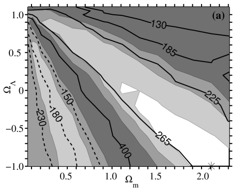
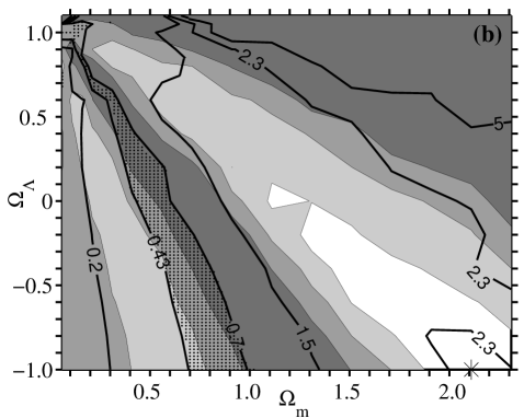
In the best-fit closed models the $\ell\simeq 200$ peak in the CMB data is fitted by the second isocurvature peak, which lies, according to Fig. 1(a), in the range $225\;\raise 1.29167pt\hbox{$<$\kern-7.5pt\raise-4.73611pt\hbox{$\sim$}}\;\ell\;\raise 1.29167pt\hbox{$<$\kern-7.5pt\raise-4.73611pt\hbox{$\sim$}}\;265$. As one might expect (see, e.g., [28] for an adiabatic analogy), now the ratio of the $\ell\simeq 200$ peak to the higher multipole $C_{\ell}$’s in the data fixes $\omega_{b}$ near the value $0.02$ in the whole best-fit band. In contrast one obtains almost no restriction for $\omega_{c}$. This is consistent with Fig. 1, where $\Omega_{m}$ can be seen to be able to take almost any value, which is then compensated by $\Omega_{\Lambda}$ to produce the correct peak position.

FIG. 3.: Angular power spectra for different models along with COBE ($\diamond$), Boomerang ($\bullet$) , and Maxima-1 ($\circ$) data. (a) Best-fit isocurvature model of Fig. 1 (solid line) and best-fit open model with LSS constraint (dashed line). (b) Best physical isocurvature fit from the fine grid (solid line) and the adiabatic reference model (dashed line). Note that up to $\ell=25$ the $\ell$ axis is logarithmic.

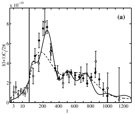
According to Fig. 3(a) the best isocurvature model ($\chi^{2}=80$) does badly with the COBE region as well as after the prominent peak. This peak is fitted quite well by the second acoustic peak while the first acoustic peak appears as a small shoulder around $\ell\simeq 80$.

The considerations so far rely on the CMB data only. However, as is well known, when discussing isocurvature models it is essential to include also the large-scale structure (LSS) data. As we will see, rough measures are already very effective in constraining the models. Therefore we make use of the the amplitude of the rms mass fluctuations in an $8h^{-1}$ Mpc sphere only, denoted as $\sigma_{8}$, which the LSS data restricts to the range $0.43<\sigma_{8}\Omega_{m}^{0.56}<0.70$ [29]. The contours of $\sigma_{8}\Omega_{m}^{0.56}$ are shown in Fig. 1(b). Apart from the upper left corner of the $(\Omega_{m},\Omega_{\Lambda})$ plane, the best-fit closed models    appear to give a far too large $\sigma_{8}\Omega_{m}^{0.56}\;\raise 1.29167pt\hbox{$>$\kern-7.5pt\raise-4.73611pt\hbox{$\sim$}}\;1.5$. This is natural, since we need a large $n_{\rm iso}$ to do away with the first peak (“the isocurvature shoulder”) at $\ell\simeq 60\ldots 100$ and to get enough power at higher multipoles. A large $n_{\rm iso}$ evidently leads to a large $\sigma_{8}$. To compensate for this, one would require a small $\Omega_{m}$. We have checked that the smaller $\Omega_{m}$ we have, the larger $n_{\rm iso}$ is allowed for by the LSS constraint. In particular, the upper left corner closed models in Fig. 1b obey the LSS constraint, although they have a rather large spectral index $n_{\rm iso}\simeq 3.1$.

On the other hand, the best-fit open models tend to have a slightly too small $\sigma_{8}\Omega_{m}^{0.56}$. These models have a relatively small $n_{\rm iso}\lesssim 2.1$, for the following reasons. (1) Since these models fit the first isocurvature peak to the $\ell\simeq 200$ peak in the data, they do not need a large $n_{\rm iso}$ to eliminate this first peak. (2) The smaller scales do not need as large a boost from $n_{\rm iso}$, since power is provided by the second peak where the data requires it. Because of this smaller $n_{\rm iso}$ these models fit the COBE region better.

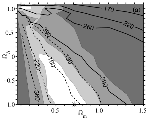
We have repeated the analysis of minimizing $\chi^{2}$ but now with the LSS constraint. As one might expect, this eliminates most of the best-fit closed models, leaving only those with a small $\Omega_{m}$ and a large $\Omega_{\Lambda}$; see the upper left corner of Fig. 2(a). The reason for this shifting of the best-fit closed-model region to the opposite corner in the $(\Omega_{m},\Omega_{\Lambda})$ plane is easy to understand. Large $n_{\rm iso}$ leads to a large $\sigma_{8}$, and hence the prior $0.43<\sigma_{8}\Omega_{m}^{0.56}<0.70$ requires $\Omega_{m}$ to be small, which in turn implies a large $\Omega_{\Lambda}$ in order to adjust the peak position.

After imposing the LSS constraint, the best-fit model is no longer a closed one but an open model at the corner of the parameter space with $\omega_{b}=0.001$ and $\Omega_{\Lambda}=-1.00$. This fit has $\chi^{2}=103$ and $(n_{\rm iso},\Omega_{m},\Omega_{\Lambda},\omega_{b},\omega_{c})=(2.05,0.71,-1.00,0.001,0.16)$. Fig. 3(a) shows that the first acoustic peak at $\ell\simeq 170$ is too low to fit the data. It is clear that the fit would further improve if one allowed for even smaller $\omega_{b}$ and $\Omega_{\Lambda}$. However, such a small $\omega_{b}$ is in clear conflict with big bang nucleosynthesis (BBN). There is some debate in the BBN community[30] on how small an $\omega_{b}$ could be acceptable. After imposing a very conservative lower limit, $\omega_{b}\geq 0.003$, our best-fit open model is already significantly worse than the best-fit closed models. Moreover, the best-fit open models have a very small, even a negative, $\Omega_{\Lambda}$. This region of the $(\Omega_{m},\Omega_{\Lambda})$ plane is disfavored by the observed supernova redshift-distance relationship[31].

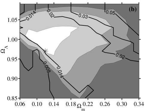
Thus we conclude that the best candidates for pure isocurvature models are the remaining best-fit closed models. These models satisfy the LSS constraint and have an acceptable $\omega_{b}$. They lie in the region of small $\Omega_{m}$ and large $\Omega_{\Lambda}$. We scanned this region with a finer grid. The resulting best-$\chi^{2}$ contours in the $(\Omega_{m},\Omega_{\Lambda})$ plane are shown in Fig. 2(b) along with the baryon density of these models. The best “physically acceptable” isocurvature fit has $(n_{\rm iso},\Omega_{m},\Omega_{\Lambda},\omega_{b},\omega_{c})=(2.80,0.12,0.97,0.015,0.074)$. The fit remains very bad, however, with $\chi^{2}=121$ for $40$ data points and $6$ parameters, to be compared to $\chi^{2}=44$ of the flat adiabatic reference model. Because of the high $\chi^{2}$ of the best fit, it is unnecessary to consider the LSS spectrum in a more detailed way. The badness of the fit is mainly due to the COBE and Boomerang data; see Fig. 3(b). The COBE contribution to $\chi^{2}$ is $2.4$ per COBE data point, the Boomerang contribution is $4.2$ per data point, while the Maxima contribution remains at $1.7$. The slope of the best-fit model is the reason for the poor fit to COBE, and although the prominent peak in the data is fitted quite well, the “flat adiabatic” peak structure of the second and third peaks in the Boomerang data leads to a conflict with the isocurvature peak structure.

As mentioned earlier, the power-law form for the power spectrum is not necessarily the most natural one in open and closed models due to the effect of spatial curvature. The curvature scale in the models studied is comparable to the Hubble scale, or larger. Thus its effect is expected to be reflected in the COBE region of the power spectrum, but not in the Boomerang/Maxima region. To assess the significance of this problem, we repeated our analysis without the COBE data points. The results remained essentially unchanged. Without the 8 COBE points we got $\chi^{2}=70$ for the best-fit model, $\chi^{2}=91$ for the best-fit with LSS constraint, $\chi^{2}=89$ for the best physically acceptable fit from the refined grid, and $\chi^{2}=40$ for the adiabatic reference model. Hence the Boomerang data alone are sufficient to rule out pure isocurvature models and our conclusions do not depend on the question of the effect of spatial curvature on the power spectrum.

Actually, since the main discriminant is the relative positions of the three peaks in the Boomerang data, which show an “adiabatic” instead of an “isocurvature” pattern, our conclusion should be independent of the shape of the primordial power spectrum as long as the observed peaks are indeed due to acoustic oscillations and do not represent features of the primordial power spectrum itself.

III summary

We have surveyed a large space of parameters for pure isocurvature models, and allowed for both open and closed universes, to find out whether there are any pure isocurvature models that fit the current CMB data better than or at least equally as well as the flat adiabatic model. There are none. We conclude that, even if one ignores the high-$z$ supernova data, pure isocurvature CDM models, including the ones with a heavily tilted spectrum, are completely ruled out by the present CMB and LSS data. Incidentally, the isocurvature models do not do too badly with the Maxima-1 data. The main CMB problems are with the COBE and the Boomerang data. To have sufficient smaller-scale power, and to suppress the first peak and boost the second peak in the closed models, a large blue tilt is needed. This leads to a slope in the Sachs–Wolfe region and reduces the largest-scale power below the level observed by COBE. The most significant problem, however, is with the Boomerang data. Boomerang shows a second and a third peak with a spacing that corresponds to a flat universe, whereas the position of the first peak in the data cannot be fitted by flat isocurvature models.