Propagation of ultra-high energy protons in regular extragalactic magnetic fields

Abstract

We study the proton flux expected from sources of ultra high energy cosmic rays (UHECR) in the presence of regular extragalactic magnetic fields. It is assumed that a local source of ultra-high energy protons and the magnetic field are all in a wall of matter concentration with dimensions characteristic of the supergalactic plane. For a single source, the observed proton flux and the local cosmic ray energy spectrum depend strongly on the strength of the field, the position of the observer, and the orientation of the field relative to the observer’s line of sight. Regular fields also affect protons emitted by sources outside the local magnetic fields structure. We discuss the possibility that such effects could contribute to an explanation of the excess of UHECR above $5.10^{19}$ eV, and the possibility that sources of such particles may be missed if such magnetic fields are not taken into account.

I Introduction

The current observations of ultra-high energy cosmic rays NagWat00 do not allow firm conclusions on the existence of the cut-off of the cosmic ray spectrum between 10¹⁹ and 10²⁰ eV, as proposed by Greisen and Zatsepin&Kuzmin GZK (GZK). The cut-off should exist if the the source distribution of UHECR were isotropic and homogeneous because of photoproduction interactions on the microwave background. There also should be BerGrig a small pile-up just before the cut-off and a secondary small dip in the spectrum due to electromagnetic pair production on the same target. While some of the highest statistics experiments HiRes_n see similar features in their data, others AGASA observe a spectrum that extends well beyond 10²⁰ eV.

The possible absence of the GZK cut-off in the observed UHECR suggests that local sources contribute a significant fraction of the observed UHECR. The spectrum that could be derived by the world UHECR statistics can indeed BBOlinto be fit fairly well with a combination of homogeneous and local source distributions. The problem with this solution is that the cosmic rays above 4.10¹⁹ eV, which should not scatter much in weak random magnetic fields, do not display strong large scale anisotropy. The observed small scale clusters asclust do not point at any known nearby astrophysical system, or at regions of increased matter density.

The isotropy of UHECR can in principle be explained by scattering in large scale magnetic fields. For example, one suggestion is Ahnetal that there is a sizable Galactic halo, similar to the heliospheric one, that isotropizes UHECR protons.

Understanding the influence of the large-scale magnetic fields on the cosmic ray propagation is vital for obtaining reliable information on the sources. The cosmic ray injection power of the sources, needed to maintain the observed highest energy cosmic ray flux, depends directly on the large-scale magnetic fields in the vicinity of the Galaxy. Magnetic fields can not only change the locally observed intensity but also the energy spectrum of UHECR Tanco98 ; SEMPR ; Deligny . Depending on the typical field strength, protons with energies greater than $10^{20}$ eV are hardly deflected during propagation whereas, for example, particles of $E=10^{18}$ eV may have a diffusive propagation pattern. In such models all cosmic rays could be local, with observed spectra strongly influenced by field geometry and source distributions.

Several earlier papers Lemoineetal97 ; Tanco98 ; Sigletal99 ; Ideetal01 have studied the acceleration and propagation of UHECR protons in intense magnetic structures. Most of these papers attempt to create quasi-realistic scenarios, making the straight-forward understanding of the involved physical processes difficult. We take the opposite approach and introduce relatively simple, yet qualitatively different, magnetic field geometries and deal with a single cosmic ray source. This makes it possible to directly follow and understand the consequences of regular large scale magnetic fields. We first assume that both the nearby UHECR source and the Galaxy are inside a wall with high concentration of matter (supergalactic plane (SGP)), which also creates a large scale magnetic field structure. Restricting our considerations to a nearby source at 20 or 40 Mpc, we study the influence of different magnetic field configurations on the particle densities, arrival directions and energy spectra.

Another scenario that we investigate is that of a source well outside the local magnetic field environment. In such a case the effects on the ‘detected’ UHECR are different, but can also be understood on the basis of the same processes that affect the local source scenario.

Before proceeding, we emphasize the following points to be kept in mind as our results are presented. The effects of our nominal field models qualitatively divide into two energy regions which, coincidentally or not, correspond to UHECR with energies above and below the GZK cutoff ($10^{19.5}$ eV). In the high energy regime the primary effect is to modestly change the direction of UHECR. The relevant experimental question is, “Can the isotropy of super-GZK UHECR be affected?” At lower energies particle propagation becomes diffusive, so that the relative geometry of source and observer in the regular magnetic field can strongly influence the UHECR spectrum and intensity. Here, the relevant question becomes, how do magnetic fields affect ones ability to infer source properties by measurements of the spectra? Third, since the transition energy is near the GZK cuto-off, the apparent strength of the GZK spectral feature may be affected by the presence of large scale non-random magnetic fields.

The outline of the paper is as follows: We discuss the supergalactic plane and field geometry in Section 2, which also gives some details of the calculation. The results on the particle densities within the 20 Mpc sphere as a function of the magnetic field geometry are presented in Section 3. The energy spectra and directions of particles leaving the 20 Mpc sphere at different angles from the magnetic field direction are given in Section 4. In Section 5 we discuss the boundary conditions of the simulation - the distance from the source to the observer, the possible existence of an external source and the time dependence of the UHE proton spectra in the case of an impulse injection of UHECR. The paper concludes with a discussion in Section 6.

II Method of calculation

We consider a single source in the supergalactic plane at a distance of 20 Mpc, compatible with the distance to the local Supercluster. This setup is motivated by the assumed matter concentration within the plane and the small number of powerful astrophysical systems in our cosmological neighborhood. The geometric structure of the calculation is illustrated in Fig. 1.

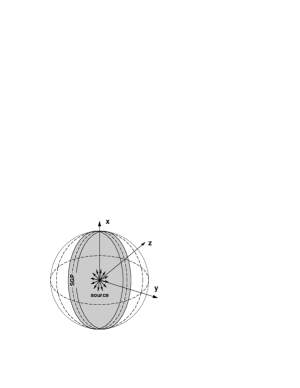
Figure 1: Geometry of the calculation in Cartesian coordinates. The supergalactic plane is infinite in $x$ and $z$ directions. Protons are injected at the origin and recorded when they cross the 20 Mpc sphere.

II.1 Magnetic field geometry

It is convenient to define the supergalactic plane as an infinite plane coinciding with the $y=0$ plane in Cartesian coordinates. The magnetic field strength of the large scale field is assumed to be constant ($B_{0}=10$ nG) up to a distance of 1.5 Mpc on both sides of the plane, i.e. the SGP has a width of 3 Mpc. At larger distances the regular magnetic field decays exponentially with a decay length of 3 Mpc.

We assume that in addition to the regular magnetic field there is a turbulent field. We take the strength of this random field to be one half that of the regular field, but never less than 1 nG. The random field is represented by a Kolmogorov expansion on three scalelengths of 1, 0.5 and 0.25 Mpc. For a discussion of the implementation of the random field see Appendix B of Ref. SEMPR .

In general it is assumed that the direction of the regular field coincides with the gravitational flow of matter, i.e. towards the supergalactic plane, and possibly along the SGP towards a higher concentration of matter in nodes, i.e. clusters of galaxies. This general idea is supported by some of the simulations of large scale structure formation Ryuetal98 We use three possible implementations of this idea:
SGP_A: The large scale field is parallel to the SGP ($B_{z}=B_{0}$, $B_{x}=B_{y}=0$).
SGP_B: The large scale field is orthogonal and points towards the SGP ($B_{y}=B_{0}$ for negative $y$ and $B_{y}=-B_{0}$ for positive $y$, $B_{x}=B_{z}=0$).
SGP_C: The field is orthogonal to SGP at distances greater than 1.5 Mpc from it (see SGP_B), and parallel to it at closer distances (see SGP_A).

A realization of our magnetic field model is illustrated in Fig. 2. Within the SGP and out to a distance $y_{reg}\sim 8$ Mpc the regular field dominates, but outside this distance the field is essentially random. Between 1.5 and 8 Mpc there is a systematic gradient to the magnetic field strength.

Figure 2: Realization of $B_{\parallel}$, the magnetic field component parallel to the large scale regular field $B_{0}$. Depending on the model $B_{\parallel}$ may correspond to $B_{z}$ (SGP_A), $B_{y}$ (SGP_B) or switch between the two at 1.5 Mpc (SGP_C). The heavy and dashed curves show the magnitude of the regular and turbulent magnetic field components, respectively.

The implementation of the regular field as an infinite plane does not allow us to close the magnetic field lines to satisfy $\vec{\nabla}\cdot\vec{B}=0$. This does not affect our results, because we are propagating the UHECR protons to distances of 20 Mpc, assuming that the field lines are closed on a larger scale.

II.2 Source spectrum and propagation

We restrict our considerations to protons as UHECR. Similar effects due to magnetic fields are obtained for heavier nuclei, if the energy is rescaled correspondingly and the differences in the energy loss are accounted for. The particles are injected at the origin of the coordinate system within a cone centered about the positive $z$ direction. The injection cone is described by its opening angle $\theta$ which may be varied according to the intended purpose. We prefer to inject particles into a cone of solid angle 2$\pi$ because in this case we can easily identify the particles that propagate in directions opposite to their injection direction.

Protons are injected with an energy spectrum

$$N(E)=\left(\frac{E}{E_{0}}\right)^{-1.25}\exp\left\{-\frac{E}{E_{\rm c}}\right\}\;,$$ (1)

with $E_{\rm c}$ = 10^21.5 eV and then usually weighted to represent an $E_{0}^{-2}$ spectrum with the same exponential cut-off. We will warn the reader for images that present results with the unweighted injection spectrum.

The particle trajectories are integrated numerically with a stepsize of 10 kpc. First the probability for photoproduction interaction is calculated, and if such an interaction takes place the photoproduction interaction is simulated by the event generator SOPHIA SOPHIA . The energy loss due to $e^{+}e^{-}$ pair production is calculated at each step and treated as a continuous process. The particle direction is calculated at each step as a function of the local magnetic field strength and direction. Neutron production and decay is taken into account. Each injected proton is followed until it crosses a 20 Mpc sphere around the injection point, or a propagation time of $1.3\times 10^{9}$ yrs has elapsed. The adiabatic losses are accounted for at every step, but starting the propagation at redshift of 0.005, which corresponds to a distance of 20 Mpc for light propagation.We expect the errors due to this procedure to be less than 10%, significantly smaller than the uncertainties in the magnetic field strength and configuration. Different numbers of particles are injected in different runs, depending on the size of the solid angle at injection and the collection area. For injection in one hemisphere ($\theta=90^{\circ}$) the typical number of calculated trajectories is $10^{6}$.

Although we solve explicitly for particle propagation in the magnetic fields, we qualitatively expect the following behaviours:
a) At the highest energies protons propagate in nearly straight lines. The gyroradius is given in Mpc by $r_{L}\simeq E_{18}/B_{-9}$ where $E_{18}$ is the proton energy in EeV, and $B_{-9}$ is the magnetic field in nG. Thus, for a 10 nG field, particles with energies above $10^{19.5}$ eV will pass through the SGP with only a modest deflection. Above $10^{20}$ eV particles propagating as neutrons will increase the effective diffusion length for UHECR.
b) Lower energy particles will be strongly affected by magnetic fields. Outside $y_{reg}$ the fields are essentially random, and propagation is isotropic and diffusive on a scale comparable to $r_{L}$.
c) For $y<y_{reg}$ the diffusion tensor is not isotropic. Diffusion is much easier along field lines than perpendicular to them, but the scaling is complicated in the region where $r_{L}$ is comparable to the coherence length $l_{coh}$ of the turbulent component of the magnetic field ZankMBM98 . The random component of the magnetic field yields a coherence length of 0.39 MpcSEMPR . We estimate that $\lambda_{\parallel}$, the diffusion length parallel to $B_{0}$, increases from $<10$ Mpc to $>100$ Mpc as the proton energy increases from $10^{18.5}$ to $10^{21}$ eV. Correspondingly, diffusion across field lines is quite inefficient, $\lambda_{\perp}\ll 1$ Mpc.
d) Although diffusion across field lines is slow, due to the large gradients in our field model there may be significant $B\times\nabla B$ drifts.

III UHECR density in different magnetic field configurations

Fig. 3 shows the projection of the particle density (i.e. density of trajectories) on the $yz$ (panel a,b,c) and $xz$ planes (panel d) for different magnetic field models. Protons are injected with the spectrum (1) in 2$\pi$ steradian with $\cos\theta$ between 1 and 0 in direction of positive $z$. The minimum injection energy is $10^{18.5}$ eV. At each propagation step of 10 kpc the position of the particle is projected to the respective plane. The particle density is dominated by the lowest energy particles not only because of the steep injection spectrum, but also because these particles are scattered more by the magnetic field and have larger pathlengths to reach the 20 Mpc sphere.

Fig. 3a shows the density projection on the $yz$ plane in the absence of any regular field. Only the random 1 nG field is present. Although the injection is restricted to the $+z$-hemisphere some of the protons scatter backwards and partially populate the backward hemisphere.

Panel b) shows the projection on the $yz$ plane for the model SGP_A, where the magnetic field is parallel to the supergalactic plane. One sees the enhancement of the proton density around the SGP. These are also mostly low energy protons trapped by the magnetic field. The ‘halo’ that fills the forward hemisphere consists of high energy particles that do not deviate significantly from the direction of injection.

Fig. 3c is for model SGP_B where the magnetic field direction follows the flow of matter to the SGP. The pattern is almost exactly the opposite to that in panel b) – at small distance from the injection point the protons are constrained to follow $B_{0}$ and in this case soon leave the SGP. When they reach $y\sim y_{reg}$ the diffusion becomes isotropic. There is also a small concentration along the SGP close to the injection point from higher energy particles injected near $\theta=0$. The density of particles crossing the 20 Mpc sphere inside the supergalactic plane is very small and consists mainly of the highest energy protons.

Fig. 3d shows the projection on the $xz$ plane for SGP_A. This is the plane that contains the magnetic field. From the perspective of cross-field diffusion the extended distribution in the $x$-direction is somewhat puzzling. Upon investigation, a correlation between $x$ and $y$ positions indicates that cross-field movement in the $x$ direction is in fact particle drift due to the gradient of the magnetic field.

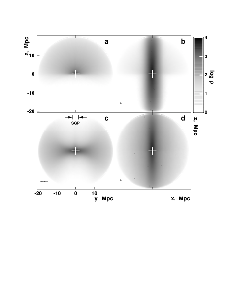
Figure 3: Particle density projections. a) projection on the $yz$ plane for random magnetic field of average strength 1 nG; b) projection on the $yz$ plane for model SGP_A; c) projection on the $yz$plane for model SGP_B; d) projection on the $xz$ plane for model SGP_A. The symbol at the lower left corner of each panel indicates the direction of the regular field.

Fig. 4 shows the projection of the particle density on the $yz$ plane for model SGP_C and the trajectory of a typical low energy particle ($E<10^{19}$ eV) projected on the same plane. The particle is injected at the origin and is immediately trapped in the SGP field. It diffuses back and forth along the plane with $\lambda_{\parallel}$ of order 5-10 Mpc (by eye), until it eventually heads off in the $y$ direction, presumably influenced by a strong random field. Once it leaves the SGP the field direction in the SGP_C model switches from $z$ to $-y$ direction. The proton is now trapped in this field, gyrates in it for a few Mpc and escapes out of the 20 Mpc sphere.

The left-hand panel shows a density pattern which qualitatively corresponds to trajectories such as that in the right-hand panel. There is a strong enhancement of the particle density in a narrow region coinciding with the SGP itself. The enhancement is stronger in the vicinity of the injection point.

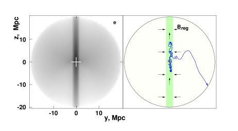
Figure 4: Right-hand panel: projection of a proton trajectory on the $yz$ plane. The arrows show the magnetic field direction outside and inside the SGP. Left-hand panel: Particle density projection on $yz$ plane for magnetic field model SGP_C.

All three models of the magnetic field configuration show qualitatively the same propagation behaviour: UHECR of energy above about 10^19.5 eV propagate almost rectilinearly, while the lower energy particles concentrate along the magnetic field lines. Because of that in the rest of this paper we concentrate on model SGP_A assuming that, although results would be different in detail, the main conclusions will still be robust.

IV Energy spectra of UHECR leaving the 20 Mpc sphere at different locations

It is reasonable to expect that the changing particle density as a function of the magnetic field model, and the location of the observer, would lead to changes in the observed energy spectrum. For example, from Fig. 3 we see that for model SGP_A the particle flux below 10¹⁹ eV will mostly escape out the end caps, ($|x|,\,|y|<1.5$ Mpc, $z=\pm 20$ Mpc) an area of order 10 Mpc². If there were no magnetic field this same flux would escape through the full 2500 Mpc² surface area of the hemisphere. Thus, an observer in the endcap region sees a flux enhanced by a factor of $\sim 100$, for energies below a few 10¹⁹ eV. Similarly, an observer who sees the source across field lines or lies outside the plane of the galaxy will see a severely reduced flux at low energies. At the same time, particles with energies above 10²⁰ eV will hardly be bent, and all observers see roughly the same flux independent of their position. Clearly, the observed spectrum of UHECR may be influenced by the presence of large scale magnetic fields. Correspondingly, effortsWaxman95 to normalize the injection power of UHECR sources by comparing to the observed spectrum at $E\sim 10^{19}-10^{19.5}$ eV are fraught with uncertainty.

To investigate this question in more detail we perform simulation runs in which we record the information for all particles that leave the 20 Mpc sphere.

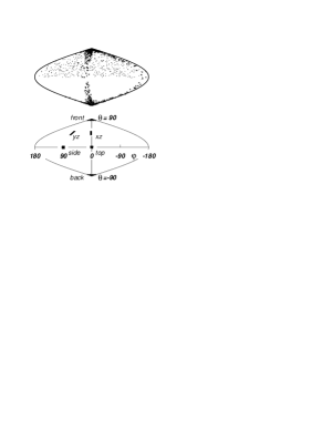
Figure 5: Upper panel: location of the exit points from the 20 Mpc sphere for protons of exit energy above (points) and below (crosses) 10^19.3 eV. The first 500 protons in each of the energy bins are plotted without weighting. Lower panel - locations of the six panels defined in the text. The vertical centerline is at y=0, x$>$0 and the outer boundary is at y=0, x$<$0.

The upper panel of Fig. 5 shows the exit points of protons subdivided in two energy groups - above and below 10^19.3 eV. The exit points reflect the particle densities shown in Fig. 4. The exit points for high energy particles map out the $2\pi$ beam of injected particles. The lower energy particles include two populations. The main population consists of particles that stay within the SGP, diffuse along field lines of the large scale magnetic field, and exit in either the $+\hat{z}$ or $-\hat{z}$ direction. The second population is particles that propagate to the edge of the SGP. These particles experience not just a large scale $\vec{B}$, but also a large scale $\nabla{B}$, and so drift across field lines. The orientation is such that protons on the positive $y$ side of the SGP drift in the $+x$ direction, whereas particles on the negative $y$ side of the SGP drift in the $-x$ direction. When projected onto the 20 Mpc sphere, the exit points for these particles define two bands, one of which intercepts the equator at $\phi\simeq 10-20$ degrees and the other at $\phi\simeq 190-200$ degrees. Note that due to the drift process, the exit points tend to be on the maximum $|y|$ excursion of the particle orbit.

The top panel of Fig. 5 shows a global picture of the exit points for two energy bins, but it does not give an adequate picture of the diversity of spectra that may be seen by an individual observer. Accordingly, we define six “caps” on the surface of the 20 Mpc sphere, each of area 3$\times$3 Mpc², at the following locations:
      front at positive $z$, $|x|,|y|$ less than 1.5 Mpc
      back at negative $z$, $|x|,|y|$ less than 1.5 Mpc
      side at positive $y$, $|x|,|z|$ less than 1.5 Mpc
      top at positive $x$, $|y|,|z|$ less than 1.5 Mpc
      yz in the forward hemisphere centered at (0, 20/$\sqrt{2}$, 20/$\sqrt{2}$)
      xz in the forward hemisphere centered at (20/$\sqrt{2}$, 0, 20/$\sqrt{2}$)
The terminology (front, back, etc.) reflects the orientation illustrated in Figure 1.

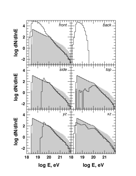
Figure 6: Energy spectra of protons that cross the 20 Mpc sphere within 9 Mpc² caps. The shaded histogram is the injection ($E^{-2}$) spectrum and the dotted histogram shows spectra propagated at 20 Mpc in the absence of magnetic fields. There is no injection spectrum within the solid angle of the back cap. See the text for the locations of the six caps.

Fig. 6 shows the spectra of the particles that leave the 20 Mpc sphere through these six caps. The shaded area shows the injected particle spectrum for the same solid angle. The dotted histogram shows the result of propagation of protons in the absence of magnetic field but including energy loss. The spectrum of particles leaving the sphere through the front cap shows the expected enhancement at energies below 10²⁰ eV. At 10¹⁹ eV the flux is enhanced by a factor of about 60. The decrease of particles above 10^20.2 eV is due to the energy loss during propagation, as can be seen by comparing to the dotted histogram. Although 20 Mpc is a cosmologically negligible distance, it is at least a factor of three higher than the mean free path for photoproduction $\lambda_{phot}$ at energies above 10²⁰ eV, which reaches a minimum of about 3.8 Mpc at 10^20.5 eV SEMPR .

The back cap only sees backscattered protons of energy below 10^19.6. In reality, for 4$\pi$ injection both the front and the back caps would see the sum of the shown two distributions. This would almost double the excess of low energy particles seen by observers connected to the source by lines of the large scale magnetic field.

All other caps show a deficit of lower energy particles. The particle spectra cut off at about 10^19.3 for the side and yz caps. Interestingly, there is a narrow enhancement in the spectrum at 10^19.5 eV. At this energy the side cap accepts protons that gyrate by either $90-\delta$ or $90+\delta$ degrees, and the exposure of the cap is effectively doubled. The two caps in the $xz$ plane above the particle source show a much more complicated spectra. The break in the spectrum occurs at higher energy than for the side and yz caps due to a longer path within the high field region of the SGP. At lower energies the spectrum is filled by a combination of particles with modest bending outside the SGP and particles that drift along the edge of the SGP. Note that the injection spectra for the side and top caps are lower by a factor of 2 since only half of the patch is exposed to the beam.

Fig. 6 demonstrates how strongly the spectrum of the observed particles from a single source depends on the relative directions of the observer and the magnetic field lines. Since the normalization point for estimates of the UHECR source luminosity is in the vicinity of 10¹⁹ eV one could easily under or overestimate the luminosity by orders of magnitude. If there are several nearby sources these effects may be somewhat ameliorated due to averaging over different geometries Tanco98 .

Fig. 7 shows velocity vector maps for the first 500 protons crossing the six caps. Protons with energy below 10^19.3 are shown with crosses and above that energy with points. The division at 10^19.3 is suggested by the spectral features in Fig. 6. Note that the entries in these scatter plots are not weighted, i.e. they represent events simulated on the flat $E_{0}^{-1.25}$ injection spectrum. For a more realistic spectrum the number of lower energy protons will increase by a factor of about 2.3 and the number of higher energy ones will decrease by a factor of about 4 compared to the population of the graph.

Figure 7: Scatter plot of the directions of protons leaving the 20 Mpc sphere through the six caps defined in the text. Protons with energy below 10^19.3 eV are shown with crosses and higher energy particles with points. The particles are not weighted and misrepresent the ratio of the fluxes in the two groups.

One might expect that, since many particles are contained within the supergalactic plane, the magnetic fields will ‘collimate’ the bunch and generate an angular anisotropy in the front and the back caps. Fig. 7 shows exactly the opposite picture - the angular distribution of the particles leaving through these two caps is very wide, if not isotropic. The reason is obvious - these particles that are contained by the magnetic field lines gyrate around them and leave the sphere with a variety of velocity vectors. The magnetic field increases the particle flux in this direction, but the particles do not point at their source. It seems that it would be best to infer the local magnetic field direction from the overall gradient in the particle flux. The situation is similar for both front and back caps. The latter one contains only three higher energy particles, which a proper weighting would eliminate from the statistics of 500.

All other caps are populated mostly by higher energy protons. The side and yz caps contain actually no lower energy events. These are the positions where the particle velocity vectors point best at their source. The average deviation from the source direction for these caps is about 15^∘ with $\sigma$ of 10^∘. These numbers are obtained with the properly weighted distribution that decreases significantly the fraction of higher energy events.

The top and xz caps show a more complicated velocity distribution. From the shape of the distribution we can conclude that it is very much influenced by drifts and bending as the protons approach the cap from a variety of angles in the ‘xy’ plane. The protons exiting through the xz cap consist obviously of two separate populations: the higher energy protons with relatively small scattering angles and the widely distributed lower energy particles that do not retain the memory of their source direction.

V The boundary conditions

The discussion so far has focused on a relatively small set of simulations, chosen to be simple enough to understand, yet complex enough to elicit behaviors which would distinguish models with large scale coherent magnetic fields. The general conclusion is that such models show effects that would complicate the process of determining source properties from observations made at a single point. Having said this, the conclusions depend on a fairly small set of models, with particular parameter values and choice of boundary conditions. It is interesting to know if the conclusions are robust with regard to these choices.

Other than geometry, the relevant parameters are the 3 Mpc thickness of the supergalactic plane, the strengths of the regular and random fields, and the rate of energy loss for UHE particles. The latter is fixed by our knowledge of particle physics and cosmology, but the others are variable. Changing parameters will alter the quantitative behavior of the simulations, but should not affect the qualitative conclusions. For example, we discern a characteristic break in behavior at energies of approximately $2\times 10^{19}$ eV, corresponding approximately to the energy at which the gyroradius is equal to the thickness of the supergalactic plane. Lowering $B_{0}$, or decreasing the thickness of the supergalactic plane, should lower the energy above which particles can effectively escape without significant bending of their trajectories. The characteristic break would remain, but its location would change.

Similarly, the relative strength of the regular and random fields determines the importance of various transport mechanisms for low and medium energy particles. As long as the regular field strength exceeds the random component, low energy particles will tend to follow the regular field within the supergalactic plane. At the edges of the plane, transport of low and intermediate energy protons is dominated by $B\times\nabla B$ drift in the $+\hat{x}$ direction if $y>0$ and oppositely for $y<0$.

Apart from such observations, we will not undertake a study of how varying parameters of our model may affect our conclusions, but instead focus on the effect of differing boundary conditions. Our simulation assumes a constant luminosity point source at the center and propagation to the edge of a sphere, after which the particles are assumed to escape. Accordingly, we examine three variations, one designed to study the boundary condition as particles exit the sphere, one which studies a different source geometry and one which studies a different source history.

V.1 Radial size of simulation

Our assumption that particles escape seems rather simplistic. Surely, a realistic model must allow for backscattering, and so an observer on the surface of the sphere would see an additional flux of particles we have not accounted for. Diffusive backflow will tend to increase the density of particles in the simulation and increase their average lifetime. On the other hand, particles that leave the simulation due to drift are not expected to return.

To address these issues, we perform another simulation run, where the 20 Mpc sphere is inside a concentric 40 Mpc sphere. We record all particles whenever they cross either sphere. The proton propagation ends when the particle crosses the 40 Mpc sphere, or when its total pathlength is longer than 400 Mpc. For the chosen injection spectrum, without weighting, there are on the average 1.12 back scatterings per injected proton and 2.08 exits from the 20 Mpc sphere. There are obviously some protons that exceed the maximum allowed propagation pathlength while inside the 20 Mpc sphere. About 90% of all injected particles leave the 40 Mpc sphere, with 4% of the injected protons exceeding the time constraint within the 20 Mpc sphere, and another 6% in the region $20<r<40$ Mpc.

Fig. 8 shows the proton crossing points for the two spheres.

Figure 8: Crossing positions in the run with two enclosed spheres. Dots show protons with energy above 10^19.3 eV, $x$’s are for protons below that energy. The particles are not weighted and only the first 500 particles in both energy ranges are plotted. See text for a better description of the different plots.

The top lef-hand panel is for protons that exit the 20 Mpc sphere for first time. This plot should be identical to the left-hand panel in Fig. 5 and it is almost identical, within the statistical uncertainty for the limited number of plotted points. The bottom left-hand panel is for protons that scatter back into the 20 Mpc sphere after they have left it. As expected, the diffusion population is still concentrated at the two poles of the distribution. Note, however, that the offset in $\phi$ for the band of drift particles is smaller for the set of reentry intersections than for the exit points. This is characteristic of drift: the particle orbit is along the drift direction in regions of low field, and retrograde in regions of high field. The reentry points are therefore closer to the SGP than the exit points. Also note that there are almost no dots in this panel, i.e. reentry of particles with energy above 10^19.3 eV. Only lower energy particles scatter back inside the 20 Mpc sphere. The top right-hand panel is for all particles that cross the 20 Mpc sphere in either direction. This is not the exact sum of the two left-hand panels since it includes particles exiting the sphere for the second (or third…) time. Also, since the statistical sample in each plot includes only the first 500 occurencies for each panel, this distribution is not the sum of those shown in the left two panels.

The bottom righ-hand plot is for the protons that leave the 40 Mpc sphere and are not followed any more in the propagation Monte Carlo. Qualitatively this map is similar to the one above it, although the number of lower energy points is relatively smaller, since the lowest energy protons are dropped from the simulation as their total pathlength exceeds 400 Mpc. The bands of drifting particles have smaller $\phi$ offsets than for the top left panel since this angle is characteristically the width of the SGP divided by the radius of the simulation.

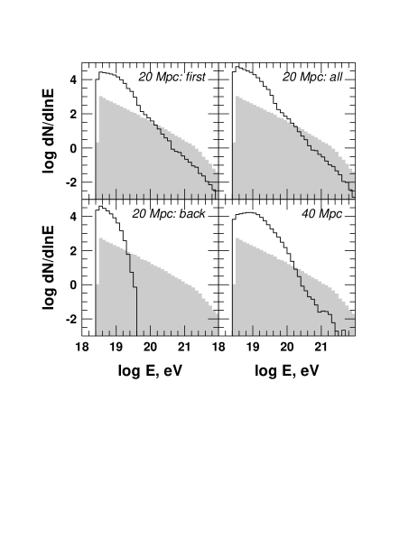
Figure 9: Energy spectra of protons crossing the front cap in the same order as in Fig. 8. The shaded histogram gives the injection spectrum in the same solid angle.

Fig. 9 shows the energy spectra of the particles that leave the spheres through the front cap under the same conditions. The top left-hand panel is for the particles that leave the 20 Mpc sphere for the first time - it has to be identical to the top left-hand panel in Fig. 6, and it is. The bottom left-hand panel is for protons that backscatter into the 20 Mpc sphere through the front cap. There is a total cutoff of the energy spectrum at 10^19.6 eV. Most of the backscattered protons are of energy below 10¹⁹ eV. The top right-hand panel shows the energy distribution of all protons crossing the front panel, independently of their direction. Since that distribution includes backscattered particles, the low energy flux is more enhanced than in the top left-hand panel here or in Fig. 6. Finally the bottom right-hand panel gives the energy spectrum of the protons that leave the 40 Mpc sphere through its front cap. Although the spectrum has qualitatively the same features as for the 20 Mpc sphere, there are some differences. The first one is that the particle flux above 10²⁰ eV is here significantly lower. This is obviously a result of the longer propagation distance and correspondingly increased energy loss. There is also some redistribution in the energy range around 10¹⁹ eV. Some of the same particles that have populated the energy range above 10²⁰ eV have moved to this range, while some of the lower energy particles are lost from the simulation because of their large pathlength. As a result, the energy spectrum is almost flat ($\sim E^{-1}$) in the range of 10^18.5-10^19.2

Our conclusion derived from the results shown in Figs. 8&9 is that the account for the backscattered particles does not change qualitatively the energy spectra of the protons leaving the 20 Mpc sphere. Doubling the propagation distance to 40 Mpc creates changes in the energy spectra that are consistent with the increased proton energy loss. Qualitatively the energy spectra measured at the two distances show similar features depending on the exit position.

V.2 External sources

A second concern is that the simulation does not account for possible sources outside the simulation volume. This is a complex problem involving the density of sources, their history and spectrum, etc. At high energy, one may presume that UHECRs will travel along nearly straight trajectories. For a mean separation of sources short compared to cosmological distances, one expects a homogeneous and isotropic phase space distribution of UHECRs. For lower energies, however, the particle horizon may be limited by diffusion Deligny , drift, or convection. In a matter dominated era, the distance between sources separates as $t^{2/3}$, where as the diffusive particle horizon grows only as $t^{1/2}$. It follows that we may observe sources in UHECRs but have no direct knowledge of the source spectra at energies below about $10^{19}$ eV. In fact, just such effects are seen in our main simulation. The front and back patches are on the same field line as the source, and see the full spectrum - even enhanced at low energies. Meanwhile the side and top patches are relatively devoid of low energy particles.

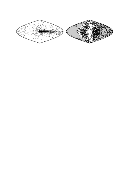
Figure 10: Exit directions (left-hand panel) and positions (right-hand panel) of protons injected by an external source. The shaded area shows the hemisphere in which the protons enter the 20 Mpc sphere.

To mock up a distant external source, we expose our simulation volume to a broad beam of protons incident on the sphere from the negative $\hat{x}$ direction, i.e. the initial phase space distribution of the protons is $\hat{n}=(1,0,0)$ and evenly distributed across the disk of radius 20 Mpc, centered at $r_{d}=(-20,0,0)$ Mpc and normal to $\hat{n}$. As in the previous tests, the injected spectrum is flat $E^{-1.25}$ so as to sample a wide variety of effects. We set $B=0$ in the region outside the simulation sphere ($r>20$ Mpc), so trajectories remain straight until they enter the simulation volume.

Figure 10 shows the exit directions and positions. As usual, the high energy particles map out the geometry. The injection velocity $\hat{n}$ is at the center of the projection in panel a). Particles of high energy pass through the sphere with a modest amount of bending in the magnetic field, creating a tail which extends in the $-\phi$ direction. In panel b), the $+x$ hemisphere is in the center of the figure, with the center line locating the SGP on the exit side of the sphere. The SGP on the entry side corresponds to the outer boundary of the projection. High energy particles are seen to exit all on the side opposite from where they enter. Those which enter in the SGP are, for the most part, deflected into the $-y$ hemisphere.

Lower energy particles show a different pattern of exit points. Those injected in the $+y$ hemisphere drift across the sphere and exit on the $+x$ side. Those injected with $y<0$ are in the region where drift is in the $-\hat{x}$ direction and, indeed, we see almost all low energy particles that exit with $y<0$ also exit with $x<0$. This is a fundamentally different behavior than is seen with the central source. In the central source simulation, particles were injected in the high field, but zero gradient, region at the center of the SGP. Low energy particles diffuse along the field lines, eventually exiting from either the front or back of the simulation volume. Only a few particles have initial energies and trajectories such that their motion is dominated by drift. For the external source, most particles are injected into the moderate field, large gradient, regions outside the SGP, where low energy particle motion is dominated by drift, as opposed to diffusion. A few low energy particles injected into the SGP, i.e. $|y|<1.5$ Mpc, tend to diffuse along field lines and also exit within the SGP, explaining the halo of exit points at the edge of the projection.

Figure 11: Energy spectra of protons crossing the patches described in the text, which are indicated in the panels with the value of the angle $\phi$.

Figure 10 shows, once again, that in the presence of coherent magnetic fields, the flux density and spectrum observed depend on the location of the observer. To illustrate this further, in Figure 11 the spectrum of particles exiting the sphere through six observer patches is shown. Since a comparison of Figs. 10 and 5 indicates that our previous set of patches are not located in regions of high particle flux, we define six patches in the $z=0$ plane which we will call by the value of the $\phi$ angle that they correspond to. Patch 0 is centered at $(x,y)=(20,0)$ and the spectrum consists only of UHE protons that manage to penetrate all the way through the SGP. Patch 180 $(x,y)=(-20,0)$ accepts mainly low energy particles injected into the SGP which exit after 1/2 gyroorbit in the SGP field. Patch 45 $(x,y)=(20/\sqrt{2},20/\sqrt{2})$ accepts both low energy particles that drift forward across the simulation volume and high energy particles that suffer mild deflections. The spectrum is similar to the injection spectrum. Patch 225 $(x,y)=(-20/\sqrt{2},-20/\sqrt{2})$ accepts mainly low energy particles which after injection drift back to exit points near their entry point. Patch 315 $(x,y)=(20/\sqrt{2},-20/\sqrt{2})$ shows an excess of high energy particles since high energy particles around 10²⁰ eV swept out of the SGP end up in this quadrant. Patch 135 $(x,y)=(-20/\sqrt{2},20/\sqrt{2})$ accepts neither high energy or low energy particles and the spectrum is suppressed at all energies, for particles exiting the simulation volume.

None of the spectra are particularly unusual, once the field geometry is accounted for, but they reinforce the conclusion that different observers will measure different spectra depending on their observation point relative to the local field geometry. The details depend on the source, as is seen by the different emphasis placed on diffusion and drift in the two simulations, but generically one requires a knowledge of field configuration in order to infer properties of the source from local observations of the particle flux.

V.3 Impulse vs. steady state

Our model assumes a steady state source, however, many models for UHECR sources are variable, episodic, or one shot explosions. It seems clear that any energy dependent transport process will result in an instantaneous observed spectrum that differs from the source spectrum. To study this we return to the central source simulation and examine the time delays as particles exit the simulation. The time delay is defined as $t_{d}=t_{exit}-t_{0}-20{\rm Mpc/c}$, with $t_{0}$ being the injection time.

Figure 12: Energy spectra of protons exiting the 20 Mpc sphere with different time delay as indicated in the panels.

Figure 12 shows the spectra of particles that exit the 20 Mpc sphere in four bins of $t_{d}$. Generally, particles that exit promptly are those with high energy, where the delays are small and only due to slight bending of the particle trajectories in the simulation’s magnetic field. Particles that exit late are particles of low energy, which have enhanced path lengths within the simulation during their diffusive transport. Figure 12 shows the spectra averaged over the whole sphere. More detailed patterns can be observed patch by patch. The main point here is that different observers, here separated in time, will observe different spectra. As before, we conclude that a program to turn observational data into statements of source spectra must take into account the possibility of organized extragalactic magnetic fields.

VI Discussion and conclusions

We propagate protons of energy above 10^18.5 eV in the presence of regular and random extragalactic magnetic fields. The propagation is limited to the cosmologically small distances of 20 to 40 Mpc. We chose to have a single particle source in order to achieve a better understanding of the proton propagation. The observers in this scheme are located on the surface of a 20 Mpc or a 40 Mpc sphere with the source in the center. The regular magnetic field is configured along a 3 Mpc wide ‘supergalactic plane’.

Our general conclusions are that the particle densities inside the 20 Mpc sphere, as well as the particle fluxes leaving the 20 and 40 Mpc spheres, depend strongly on the relative positions of the observers to the magnetic field directions. Lower energy particles are captured and channeled through the ‘supergalactic plane’ both in the direction parallel and antiparallel to the magnetic field.

To quantify better the energy spectra of the protons leaving the 20 Mpc sphere in different locations we position several caps at different angles and distances from the magnetic wall. At the exit from the 20 Mpc sphere inside the magnetic wall and on the same field line as the source (the caps front and back in Fig. 6) the proton flux at around 10¹⁹ eV exceeds the injection spectrum by almost two orders of magnitude.

For particles exiting through caps that are at positions normal to the magnetic field direction and the SGP (side and yz), there is a lack of lower energy particles. Those of energy below about 10^19.3 eV, that are enhanced in the first two caps, are depleted since they lack the magnetic rigidity to cross field lines to reach these caps.

The energy spectra in caps top and xz show intermediate spectra. Although direct propagation into these patches is strongly suppressed at low and intermediate energy, these caps capture a population of particles that drift along the edges of the SGP. Overall we could not find a position on the 20 Mpc sphere where the energy spectrum of the exiting particles resembled the injection spectrum.

The fluxes of particles above 10²⁰ eV are only mildly affected by the position of the observer. Only a small fraction of these particles are contained in the ‘supergalactic plane’ and the corresponding flux enhancement is minimal. Although reproducing the source beam pattern, the spectrum in this region is strongly affected by energy loss processes due to scattering off the cosmic microwave background.

The change in the flux density does not translate into anisotropic angular distribution for the particles that leave the 20 Mpc sphere along the magnetic field lines. The lower energy particles that are contained by the magnetic structure gyrate around the field lines and arrive at the front cap with almost isotropic angular distribution. Some degree of anisotropy can be seen at other locations that are reached only by higher energy protons. Even there the particle arrival angles do not coincide with the source direction and are strongly influenced by secondary propagation effects, such as drifts.

In order to study the possible ‘edge effects’ related to the short propagation distance and the existence of only a single source, we propagate protons in a larger, 40 Mpc sphere, concentric to the primary one. All protons that cross the 20 Mpc sphere, independent of their direction, are recorded, as well as those that leave the 40 Mpc sphere. The comparison between the positions in which the protons leave the two spheres and the energy spectra at the sphere crossings show qualitatively similar pictures. In both cases the lower energy particles are confined to the ‘supergalactic plane’ where the particle fluxes are significantly higher. The addition of the backscattered protons to the front cap at 20 Mpc increases the 10¹⁹ eV excess over the injection spectrum. The energy spectrum of protons that leave the 40 Mpc hemisphere through its front cap is influenced by the additional propagation distance, but with similar qualitative features.

We also study the effects of the magnetic field on protons injected by an external source by simulating the propagation of a plane front of protons moving in direction $\hat{x}$ = (1,0,0). The quantitative effects in this scenario are different from these of a central source, but they are still caused by the proton motion in the magnetic field and generate significant angular deflection and changes in the ‘detected’ proton energy spectra.

If the UHE protons are injected by an impulsive process, such as a gamma ray burst in the center of the 20 Mpc sphere, the proton exit spectrum depends heavily on the time delay after the burst. The fast particles arrive first, while the low energy ones suffer delays up to, and occasionally exceeding 1.3$\times$10⁹ yrs.

There are three reasons for performing the research that we described. First, the presence or absence of a GZK cut-off is considered fundamental to understanding the sources and propagation of UHECR. The results presented here suggest that the possible presence of large scale 10 nG fields complicates the interpretation of UHECR data. The second one is related to the derivation of the UHECR source luminosity, which is usually done in the vicinity of 10¹⁹ eV. The simulations that we performed emphasize the importance of accounting for the possible existence of ordered extragalactic magnetic fields. In their presence, the energy spectrum of particles emitted from a cosmologically nearby source depends very strongly on the relative position of the source and observer to the direction of the ordered magnetic field. Neglecting these fields could lead to big errors in the estimate of the UHECR luminosity.

The third reason is a study of the correlation between particle fluxes and arrival direction distribution. Even in the case of a single UHECR source, which we discuss in this paper, we could not find such a correlation, except for the highest energy protons. The enhanced particle fluxes in directions parallel to the magnetic field are almost isotropic, because of the gyration of the protons around the magnetic field lines. An observer in the front cap would not be able to recognize the direction of our single source, except in the case of very large experimental statistics. Only by the observations of cosmic rays of energy exceeding 10²⁰ eV one would be able to see some clustering around the source direction.

The dividing energy between diffusive and almost rectilinear propagation in our calculations is of order 10^19.3 eV. There are some experimental indications, based on a part of the world UHECR statistics Stanevetal95 that there is an increase in the anisotropy of these particles at energies above 10^19.6 eV. If this or a similar observation is confirmed in the future, it would suggest the existence of ordered magnetic fields of order 20 nG in our cosmological neighbourhood.

Our main conclusion is that the energy spectra and angular distribution of protons accelerated both at a nearby or at a distant source are strongly affected by modest regular extragalactic magnetic fields. This is valid independently of the model for UHECR production. Thus, it is important to allow for the possibility of large scale magnetic fields in UHECR data analysis and source searches. On the other hand, if a source of UHECR in a relatively wide energy range is identified in the nearby Universe, and high experimental statistics exist as expected from the currently active and future experiments HiRes ; Auger ; EUSO ; OWL , one could study the strength and geometry of extragalactic magnetic fields that are not accessible in any other way, utilizing techniques suggested by this research.

Acknowledgements The authors acknowledge fruitful discussions with P.L. Biermann, P.P. Kronberg, W. Matthaeus and J.W. Bieber. This research is supported in part by NASA Grant NAG5-10919. RE&TS are supported also by the US Department of Energy contract DE-FG02 91ER 40626.

References

- (1) M. Nagano & A.A. Watson, Rev. Mod. Phys. 72, 690 (2000).
- (2) K. Greisen, Phys. Rev. Lett. 16, 748 (1966); G.T. Zatsepin & V.A. Kuzmin, JETP Lett. 4, 78 (1966).
- (3) V.S. Berezinsky & S.I. Grigoreva, Astron. Astrophys., 199, 1 (1988).
- (4) T. Abu-Zayyad et al., Phys. Rev. Lett., submitted, astro-ph/0208243
- (5) M. Takeda et al., Phys. Rev. Lett., 81, 1163 (1998); N. Sasaki et al., Proc. 27th ICRC (Hamburg) 1, 333 (2001); for updates of the experimental results see http://www-akeno.icrr.u-tokyo.ac.jp/AGASA/
- (6) M. Blanton, P. Blasi & A.V. Olinto, Astropart. Phys., 15, 275 (2001)
- (7) Y. Uchihori et al., Astropart. Phys., 13, 151 (2000).
- (8) P.L. Biermann et al., Nucl. Phys. B (Proc. Suppl.), 87, 417 (2000)
- (9) G.A. Medina Tanco, Ap. J., 505, L79 (1998).
- (10) T. Stanev et al, Phys. Rev. D62: 093005 (2000).
- (11) O. Deligny, A. Letessier-Selvon & E. Parizot, astro-ph/0303624
- (12) M. Lemoine et al., Ap. J., 486, L115 (1997)
- (13) G. Sigl, M. Lemoine & P.L. Biermann, Astropart. Phys., 10, 141 (1999).
- (14) Y. Ide et al, Publ. Astr. Soc. Japan, 53, 1153 (2001)astro-ph/0106182.
- (15) D. Ryu, H. Kang & P.L. Biermann, Astron. Astrophys., 335, 19 (1998).
- (16) A. Mücke et al., Comp. Phys. Comm. 124, 290 (2000).
- (17) G.P. Zank, et al, J. Geophys. Res. 103, 2085 (1998).
- (18) E. Waxman, Ap. J. 452, L1 (1995)
- (19) P.P. Kronberg, Rep. Prog.Phys. 57, 325 (1994).
- (20) T.E. Clarke, P.P. Kronberg & H. Böringer, Ap. J., 547, L111 (2001).
- (21) T. Stanev et al., Phys. Rev. Lett., 75, 3056 (1995).
- (22) T. Abu-Zayyad et al., Proc. 26th Int. Cosmic Ray Conf. (Salt Lake City, Utah), eds. D. Kieda, M. Salamon & B. Dingus, 5, 349 (1999).
- (23) M. Boratav et al., Proc. 25th Int. Cosmic Ray Conf. (Durban) eds. M.S. Potgieter, B.C. Raubenheimer & D.J. van der Walt, 5, 205 (1997).
- (24) The current status of the EUSO proposal is displayed at www.ifcai.pa.cnr.it.
- (25) L. Scarsi et al. in Proc. 26th ICRC (Salt Lake City, Utah), eds. D. Kieda, M. Salamon & B. Dingus, 2, 384 (1999).