Quiet Sun coronal heating: analyzing large scale magnetic structures driven by different small-scale uniform sources.

Recent measurements of quiet Sun heating events by Krucker & Benz (Krucker98 (1998)) give strong support to Parker’s (par (1988)) hypothesis that small scale dissipative events make the main contribution to the quiet heating. Moreover, combining their observations with the analysis by Priest et al. (pr1 (2000)), it can be concluded that the sources driving these dissipative events are also small scale sources, typically of the order of (or smaller than) 2000 km and the resolution of modern instruments. Thus arises the question of how these small scale events participate into the larger scale observable phenomena, and how the information about small scales can be extracted from observations. This problem is treated in the framework of a simple phenomenological model introduced in Krasnoselskikh et al. (KPL (2001)), which allows to switch between various small scale sources and dissipative processes. The large scale structure of the magnetic field is studied by means of Singular Value Decomposition (SVD) and a derived entropy, techniques which are readily applicable to experimental data.

1 Why small-scale sources ?

The anomalously high temperature of the solar corona is still a puzzling problem of solar physics, despite the considerable theoretical and experimental efforts involved for a long time (e.g. Priest et al., pr1 (2000); Einaudi & Velli, Einn (1994)). Since the energy release in the largest heating events (flares and microflares) does not supply enough power to heat the Corona, the statistical behavior of smaller-scale and less energetic but much more frequent events is an essential feature of the problem, as was conjectured some time ago by Parker (par (1988)).

An important result that supports Parker’s hypothesis was reported by Krucker & Benz (Krucker98 (1998)) who have found from the Yohkoh / SXT observations, assuming that the flaring region has a constant height, that the energy probability density has the form of a power law in the energy range $10^{24}$–$10^{26}$ ergs with an exponent about $-2.59$. Such an exponent less than $-2$ indicates that heating takes place in small scales, while on the contrary an exponent greater than $-2$ indicate that large scale phenomena play a dominant role. The conclusion of Krucker & Benz was confirmed by Parnell & Jupp (Parnell00 (2000)), who estimated the exponent to be between $-2$ and $-2.1$ making use of the data of TRACE and supposing that the height varies proportionally to the square root of the area. The relatively steep slope of the energy distribution found by these authors also suggests that the smallest flares contribute essentially to the heating. Mitra & Benz (Mitra01 (2000)) have discussed the same observations as Krucker & Benz but supposing the height variations similar to Parnell & Jupp, they have shown that the exponent becomes a little larger then previous estimate but still is smaller than minus two.

Making use of the multi-wavelength analysis Benz & Krucker (Benz99 (1999)) have shown that energy release mechanisms are similar in large scale loops and in the faintest observable events. They have also noticed that the heating events occur not only on the boundaries of the magnetic network but in the interiors of the cells also. Priest et al. (Priest98 (1998)), comparing model predictions for the plasma heating in the magnetic loop due to the distributed energy source with observations led to the conclusion that the heating is quasi-homogeneous along the magnetic loop. This means that the heating process does not occur in the close vicinity of the foot points but rather in the whole arc volume. Putting together these facts, it follows that the characteristic spatial scale of the magnetic field loops which supply the magnetic field dissipated is of the same order as the characteristic scale of the dissipation. Thus we may conclude that not only the dissipative process, but also the energy sources have small characteristic length. It also results from these observations that the sources are distributed quite homogeneously in space.

Hence it is important to discuss the role and properties of sources and dissipative processes in the framework of simplified models. Such an approach allows to study the correspondence between large scale magnetic field properties and characteristics of the small scale (eventually smaller than the experimental resolution) characteristics of sources and dissipative events, which may become a basis of the analysis of experimental data, helping to explain the nature of the physical phenomena underlying the observations.

A phenomenological model allowing for different sources and physical dissipation mechanisms was proposed in Krasnoselskikh et al. (KPL (2001)), and their effect on the temporal statistics of the total dissipated energy were studied. This model is briefly discussed in the next section. To study spatial properties of the magnetic fields and dissipative events, detailed statistical tests applicable both to simulations and experimental data are required. Tools such as the magnetic field entropy and extraction of the most energetic and large scale spatial/temporal eigenmodes by means of Singular Value Decomposition (SVD) are described in section III. Their application to our model and their ability to discriminate between various sources and dissipative mechanisms are discussed in section IV, and the final section proposes a review and a critical discussion of the results.

2 Small-scale driving and dissipation

Various phenomenological models of flare-like events and cooperative phenomena in the corona have been considered in the literature (e.g. Lu & Hamilton, Lu-H (1991); Vlahos et al., vlah2 (1995); Georgoulis et al., Georg4 (2001)), mostly relying on the notion of Self-Organized Criticality (Jensen, Jensen (1998)). Such models usually exhibit infinite-range spatial correlations, and due to the tenuosity and localization of the driving do not provide an appropriate framework for our purpose.

Instead, we shall use the model introduced in (Krasnoselskikh et al., KPL (2001); Podladchikova et al., PKL (1999)) which allows for a driving more distributed in space and dissipative processes relevant to heating studies. As usual, the model represents a simplification of the magnetohydrodynamic induction equation

$$\frac{\partial\mathbf{B}}{\partial t}=\mathbf{\nabla}\times(\mathbf{u}\times\mathbf{B})+\mathrm{dissipative\ term.}$$ (1)

The turbulent photospheric convection randomizes in some sense the first term of the right hand side, which can be replaced by various source terms with specified statistical properties. The dissipative terms may take into account different effects such as normal and anomalous resistivity or magnetic reconnection, which in general depend on the current density and magnetic field configuration (their meaning and differences between the two in this context are discussed at length in Krasnoselskikh et al. (KPL (2001)).

The model is two-dimensional, the magnetic field being perpendicular to the grid, with periodic boundary conditions. A discrete description of the magnetic field in term of cells is proposed, while the currents are computed from

$$\left(\begin{array}[]{c}j_{x}\\ j_{y}\end{array}\right)=\frac{1}{\delta}\left(\begin{array}[]{c}B\left(x,y\right)-B\left(x,y+\delta\right)\\ B\left(x+\delta,y\right)-B\left(x,y\right),\end{array}\right)$$

where $\delta$ is cell length ($\delta=1$ in the following). The currents can be considered as propagating on the border between the cells, and satisfy Kirchoff’s law at each node.

As discussed in the introduction, one may suppose that the source term representing the magnetic energy injection has a characteristic spatial comparable with that of the dissipative processes. Hence source terms, mimicking the magnetic energy injection from the turbulent photosphere, are assumed to have a vanishing average, and act in each cell of the grid at each time step. Three different types with different statistical properties are considered:

• Random sources. The simplest source is given by independent random variables $\delta B$ in the set $\{-1,0,1\}$, acting in each cell. Such a source can be made dipolar by dividing the grid into two parts where random numbers are chosen from the similar set that have however, positive and negative mean values, respectively, for each of these parts.

• A chaotic source. Turbulence is certainly not a completely random process, and some of its aspects are enlightened by deterministic models. The source in each cell evolves independently of others according to

  $$\delta B_{n+1}=1-2(\delta B_{n})^{2},$$

  where $\delta B\in[-1;1]$, which is an instance of the logistic (Ulam) map, well known for its chaotic properties.

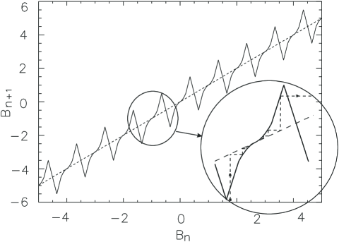
• Geisel map source. The source term may depend on the value of $B$ itself. When the dissipation is absent, the magnetic field in each cell evolves according to a map

  $$B_{n+1}=f(B_{n}).$$

  We used the map introduced by Geisel and Thomae, (Geisel (1984)), hereafter called Geisel map (see Fig. 1), whose marginally stable fixed points are responsible for the anomalous diffusion exhibited by this map

  $$\langle B^{2}\rangle\propto t^{\alpha},\quad\alpha<1.$$

  It is generally expected that magnetic field lines in a turbulent plasma exhibit a subdiffusive behavior, which is, however, more complex than described above.

Figure 1: Graphical representation of the Geisel map (solid line). The fixed points of the map correspond to the intersections of the graph with the straight line $B_{n+1}=B_{n}$ (dashed line).

It is worth pointing out that all the source evolve in time in each cell independently of other cells, and that interaction between the fields in neighboring cells are only related with the dissipation effects.

The dissipation provides the conversion of magnetic energy into particle acceleration and thermal energy, and in our model provides the coupling between the magnetic field elements. Dissipative processes are most important where a current sheet carrying strong current density has formed. Neglecting resistivity, which is small in the corona, one is left with various instabilities of magnetic field configurations which can provide the dissipation. We consider two of them:

• Anomalous resistivity, which arises from the development of certain instabilities such as modified Buneman when the electric current exceeds a certain threshold in collisionless plasma. In our model the currents are simply annihilated whenever they exceed a certain threshold,

  $$|j|\geq j_{\max}.$$

• Reconnection, for which we impose which in our model the additional requirement that the magnetic field has a configuration favorable to a X-point. Hence, the following two conditions should be satisfied simultaneously:

  $$|j|=|B-B^{\prime}| \geq j_{\max},$$

  $$B\cdot B^{\prime} < 0,$$ (3)

  The new condition results in the existence of currents that can strongly overcome the critical value.

The difference underlined here is mainly that reconnection represents a change in equilibrium, from one topology (here a X-point) to another, while anomalous resistivity does not require any particular topology and thus may also act in cell interiors and not only at boundaries. Another important difference is that anomalous resistivity provides Joule-like heating, while reconnection yields accelerated outgoing flows and thus may be associated to non-thermal radiation.

When the current is annihilated, magnetic field values in both neighboring cells, $B$ and $B^{\prime}$, are replaced by $1/2(B+B^{\prime})$, so the density of magnetic energy dissipated in a single event is given by

$$\Delta E=\frac{1}{4}\,(B-B^{\prime})^{2}=\frac{1}{4}\,j^{2}\gtrsim\frac{1}{4}\,j_{\max}^{2}.$$

The procedure modeling the dissipation of currents is the same for both anomalous resistivity and reconnection. On each time step, the currents satisfying the dissipation criterion are dissipated till all the currents become subcritical (or have the same sign for the case of reconnection). Then, we proceed to the next time step and switch on the source. Indeed, dissipative processes are supposed to be faster than the driving ones. The total dissipated energy is calculated as a sum over all the dissipated currents for the time step considered.

In Podladchikova et al. (PKL (1999)) and Krasnoselskikh et al. (KPL (2001)), the influence of the dissipative processes and source terms on the statistical properties of the dissipated energy was studied. The dissipation was shown to have a significant influence on the statistics of dissipated energy. Indeed the reconnection mechanism was shown to yield the strongest deviation from Gaussian distribution in the large energies. However, the probability density of the dissipated energy was shown to be rather insensitive to the nature of the magnetic field sources. In this paper we would like to explore further the dependence of the large scale magnetic field statistical properties upon the physical characteristics of the source and dissipation processes in the framework of our model. The aim of this work is to investigate the possibility of getting information about small scale magnetic energy sources making use the large scale magnetic field. In order to do so, we study hereafter the spatial complexity of the large scale field by means of spatial correlations, entropy and eigenmodes (Singular Value Decomposition).

3 Characterization of spatial complexity

Spatial complexity can be characterized in many different ways (e.g. Grassberger, Grassberger86 (1986)). Linear properties are traditionally studied by considering the time averaged spatial correlation function

$$C({\mathbf{r}})=\langle B({\mathbf{x}},t)\;B({\mathbf{x}+r},t)\rangle_{{\mathbf{x}},t}/\langle B({\mathbf{x}},t)^{2}\rangle_{{\mathbf{x}},t}\ ,$$ (4)

where the average is carried out over different positions and times (or events). We have computed the characteristic decay length of this correlation function for various sources, dissipation mechanisms, and thresholds.

A different approach, which is used in the framework of image processing, is based on the Singular Value Decomposition (SVD) or Karhunen-Loève Transform, see Golub & van Loan (Golub96 (1996)). For each time step, the bivariate magnetic field intensity $B(x,y)$ can be viewed as 2D image. We decompose this image into a set of separable spatial modes

$$B(x,y)=\sum_{k=1}^{N}\mu_{k}\;f_{k}(x)\;g_{k}^{*}(y)\ .$$ (5)

By making these modes orthogonal $\langle f_{k}f_{l}^{*}\rangle=\langle g_{k}g_{l}^{*}\rangle=\delta_{k,l}$, the decomposition becomes unique. The weights $\mu_{k}$ of these modes, also called singular values, are conventionally sorted in decreasing order, and are invariant with respect to all orthogonal transformations of the matrix $B(x,y)$. In our case, the number $N$ of modes is equal to the spatial grid size.

A key property of the SVD is that it captures large-scale structures in heavily weighted modes, whereas patterns that are little correlated in space are deferred to modes with small weights. The distribution of the singular values is therefore indicative of the spatial disorder: a flat distribution means that there is no characteristic spatial scale and hence, the magnetic field should not show large-scale patterns. Conversely, a peaked distribution suggests that there are coherent structures (Dudok de Wit, DdW95 (1995)). It must be stressed that this approach is, like the previous one, based on second order moments only, since the spatial modes and their singular values issue from the eigenstructure of the spatial correlation matrix of the magnetic field.

From the SVD modes of the 2D magnetic field, one can define a measure of spatial complexity, which is based on the SVD entropy (Aubry, Aubry91 (1991)). Let $E_{k}=\mu_{k}^{2}/\sum_{i}\mu_{i}^{2}$ be the fractional amount of energy which is contained in the $k$’th mode. The SVD entropy can then be defined as

$$H=-\lim_{N\rightarrow\infty}\frac{1}{\log N}\sum_{k=1}^{N}E_{k}\log E_{k}\ .$$ (6)

The maximum value $H=1$ is reached when spatial disorder is maximum, that is when $E_{k}=1/N$ for all $k$. $H=0$ means that all the variance is contained in a single mode.

The SVD can also be used as a linear filter to extract large scale patterns from a background with small scale fluctuations. To do so, one should perform the SVD and then in eq. 5 sum over the strongest modes only, to obtain a filtered magnetic field. There is obviously some arbitrariness involved in the identification of what we call strong modes, but the process can be automated by using robust selection criteria, see for example Dudok de Wit (DdW95 (1995)).

4 Spatial complexity and properties of the source and dissipation

4.1 Spatial correlations

Figure 2: Correlation length dependence on the threshold of dissipation for both dissipation rules. Anomalous resistivity is marked by triangles, reconnection by squares.

Figure 3: Averaged magnetic field spatial correlation coefficient in log-linear plot (solid lines). Dotted lines represent the best fits by exponential function. The results are obtained for random and subdiffusive sources with a threshold of dissipation $j_{\max}=1$. a) random source, anomalous resistivity dissipation, correlation length $L=17$; b) random source, reconnection dissipation, correlation length $L=19$; c) subdiffusive source, anomalous resistivity dissipation, correlation length $L=23$; d) subdiffusive source, reconnection dissipation.

Figure 4: Typical magnetic field for random source and reconnection, with $j_{\max}=1$. a) Magnetic field at $t=1000$, with entropy $H=0.79$; b) Zoom of the precedent image; c,d) filtered magnetic field, with 20 eigenmodes, at $t=1000$ and $t=2000$ ($H=0.807$).

Figure 5: Magnetic field for the subdiffusive source and reconnection, with $j_{\max}=1$. a) Magnetic field in a transient state, $H=0.73$; b), Magnetic field in a stationary state, $H=0.51$ c) 20 modes of the precedent image; d), magnetic field at $t=3000$, $H=0.527$

Spatial correlation function as defined by Eq. 4 were averaged in time after the system has reached a stationary state.

For the small grids, of the order of $30\times 30$, the correlation function decays as a power-law. It was shown in Krasnoselskikh et al. KPL (2001) the probability density of the total dissipated energy also decays as a power-law in this case. However the resemblance to a self organized critical behavior is only an artifact of the small grid size, when the correlation length is comparable with the grid size, and disappears for large enough grids. Indeed, for grid sizes around $100\times 100$ (or greater), the time averaged correlations functions have an almost exponential decay, while the dissipated energy has a quasi-Gaussian distribution.

In case of exponential correlation functions, a correlation length is easily defined as the parameter $L$ such that

$$C(r)=\exp(-r/L).$$

We have found in our simulations that the correlation length $L$ remains almost constant when the grid size is increased above $200\times 200$, and furthermore that $L$ is much smaller than the linear grid size. In such a case, it is legitimate to expect that results do not depend significantly on the grid size or boundary conditions. In the remainder of this paper all results are presented for a grid $400\times 400$ and a small threshold is used ($j_{max}=1$, which is of the order of $\sqrt{\langle\delta B^{2}\rangle}$).

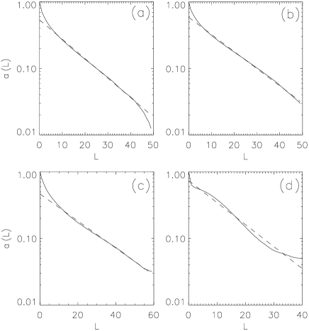
As shown on Fig. 2, for the random magnetic field source the average correlation length is larger for the reconnection type dissipation than for anomalous resistivity. This can be explained by the presence of supercritical currents $>j_{\max}$ which may exist because of condition (3). Moreover in both cases the correlation lengths are decreasing functions of $j_{\max}$ (see Fig. 2). These results are hardly changed if the random source is replaced by the Ulam map source (see previous section). Only in the case of a magnetic field following the Geisel map, and when dissipative processes are ruled by anomalous resistivity (Fig. 3c), the average correlation length is a little bit larger than in the previous cases (see Fig. 3ac). When dissipation occurs through reconnection, the average correlation function seems featureless (see Fig. 3d) (to the least neither exponential nor power-law), and no correlation length can be unambiguously computed for comparison with previous results.

Thus the correlation function seems to have difficulties here in indicating significant differences between the different processes. However, strong differences are seen simply by visible inspection of the magnetic field between for example the random and Geisel map sources (Figs. 4b and Figs. 5b). Hereafter we shall present an alternative analysis using the spatial entropy defined in terms of SVD eigenvalues.

4.2 Singular values and coherent spatial modes

As discussed in the previous section, the Singular Value Decomposition provides an orthogonal decomposition which allows to extract coherent patterns eventually existing in the bivariate magnetic field at a given time.

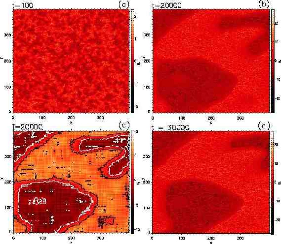
In our case, the distribution of singular values appears to be significantly peaked (Fig. 6), showing that the bi-dimensional wavefield is dominated by a few spatial modes. For instance, the most energetic mode ($f_{1}(x)$, in the notation of Eq. 5 obtained from SVD of the magnetic field for a Geisel source and dissipation by reconnection clearly corresponds to a large scale coherent structure (Fig. 7).

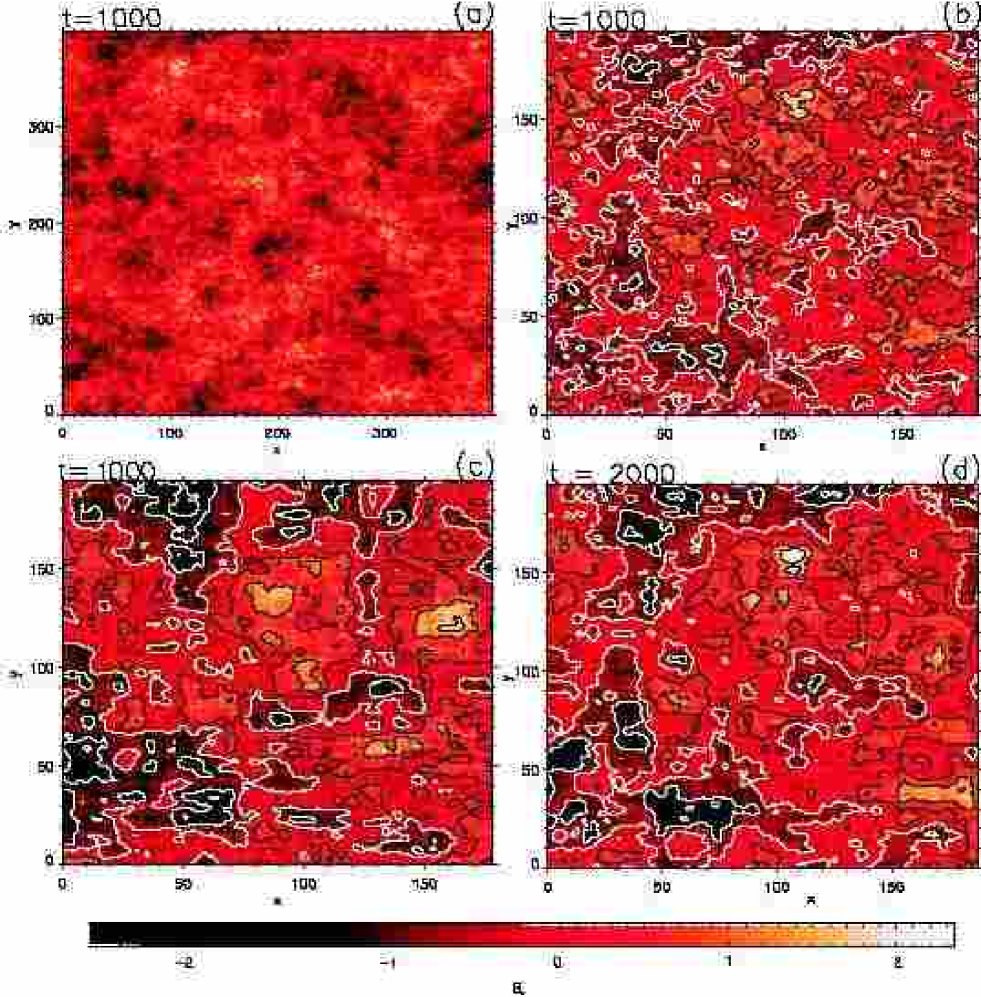
The fact that the most heavily weighted modes correspond to large scale magnetic field structures is further illustrated by Figs. 4 and 5, by comparison of the magnetic field (Figs. 4b and 5b) with an approximation of the magnetic field containing only 20 modes (Figs. 4c and 5c) which has a very similar large scale structure. In both cases, the retained modes correspond to the fast exponential decay of the strongest singular values, down to the turning point where the decay becomes slower (as in Fig. 6), and the following singular values are filtered out and set to 0 before the inverse SVD is performed. In particular, it is clear that the large scale structure of magnetic field appearing with Geisel map sources, and not with random sources, is retained by SVD (Fig. 5).

However, this analysis provides only a decomposition of the magnetic field at a given time, and no information about the lifetime of these structures which is quite crucial though. Monitoring the time evolution of the system, it appears that the heavily weighted modes appear to persist for long times, as can be seen comparing the filtered magnetic field at two times separated by 2000 time steps (Figs 5c and d). Actually, it is seen on Figs 5a,b,c how these structures grow from the initially disordered state.

Figure 6: Energy of the spatial eigenmodes of magnetic field formed by subdiffusive source and reconnection dissipation.

Figure 7: Most energetic spatial mode $f_{1}(x)$ obtained by the same Singular Value Decomposition as in Fig. 6.

Figure 8: Averaged temporal correlation function of the magnetic field (solid lines) in log-linear plot calculated from $4\times 10^{4}$ times steps. Dotted lines represent the best fits by an exponential function. The results are obtained for random and subdiffusive sources, reconnection dissipation, with a threshold of dissipation $j_{\max}=1$. a) random source, correlation time $\tau=202$; b) the same as previous, but only for the first 20 modes, $\tau=220$; c) subdiffusive source, $\tau=1435$; d) the same as (c), but only for first 20 modes, $\tau=2958$.

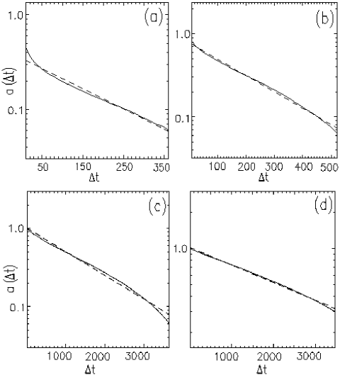
Thus the coherent structures extracted by SVD have a long lifetime and produce a slow decay of the temporal autocorrelation function, defined by

$$C(\tau)=\langle B(x,y,t+\tau)B(x,y,t)\rangle_{x,y,t},$$

as shown in Fig. 8. While small-scale structures rapidly appear and disappear, the large scale ones evolve slowly. In that sense, they are truely coherent structures.

4.3 Magnetic field entropy

Quantitatively, the coherence degree of the magnetic field can be measured by the spatial entropy defined by Eq. 6 from the singular values. This definition involves a limit $N\rightarrow\infty$, but in practice, for large enough grid sizes, it can be checked that the quantity computed for a $N\times N$ subset of $B$

$$H_{N}=-\frac{1}{\log N}\sum_{k=1}^{N}E_{k}\log E_{k}$$

converges toward a well-defined limit as $N$ increases. Computing the entropy $H_{N}$ for increasing $N$, we have obtained the curves displayed on Fig. 9 which show that the entropy already converges for matrix sizes about $100\times 100$, although it seems that the convergence is faster for the subdiffusive source than for the random source. Thus we may conclude that, provided large enough grids are considered, the entropy $H$ is fairly independent of the grid size.

Figure 9: Partial entropies $H_{N}$ as a function of the grid size $N$. The continuous line is for the subdiffusive source, and the dashed one for the random source. This entropy is normalized so that $H=1$ corresponds to maximum disorder.

The entropy has a monotonous decay in time and converges toward a finite value in the steady state (see Tab. 1), indicating the simultaneous decrease of spatial complexity and the formation of slowly evolving large scale magnetic field structures.

t	$100$	$500$	$20000$	$30000$
H	0.73	0.69	0.51	0.527

Table 1: Variation of the entropy in time, for the subdiffusive source and reconnection (see also Fig. 5).

The major result here is that the value toward which the entropy converges in time exhibit significant differences between the different sources are used, as summarized in Table 2.

source type	H
random	0.8
Ulam	0.78
Geisel	0.53

Table 2: Entropy in the steady state for various source types, and dissipation by reconnection.

5 Conclusion and discussion

To study coronal heating due to dissipation of small-scale current layers, we have performed a statistical analysis of a simple model. The model was introduced in Krasnoselskikh et al. KPL (2001), and its principal difference with previous ones is that the system is driven by small scale homogeneously distributed sources acting on the entire grid for each time step. The idea to consider small scale sources is motivated by observations by Benz & Krucker (Benz98 (1998, 1999)) that the heating occurs on the level of the chromosphere, thus the magnetic field structures, dissipation of which supplies the energy for the heating, are also of a small scale.

The question addressed in this paper was the following: if the actual measurements cannot resolve the characteristic scale of the heating, in what sense are the ”macroscopic” observable properties influenced by the properties of the smaller scale sources ?

To this purpose we have carried out the comparative analysis of statistical estimations the large scale spatial characteristics of the magnetic field such as the correlation length, entropy and most energetic eigenmodes for the different source types that were used in the model (random, chaotic and intermittent with anomalous temporal diffusion).

The ”noisy” small scales were filtered out in order to study large scale of the magnetic field. For this purpose we have reconstructed the magnetic field from eigenmodes given by SVD that corresponds to most energetic coherent structures. The less energetic modes that corresponds to noise level were truncated.

The results can be summarized as follows:

The large scale spatial characteristics of the magnetic field such as the correlation length, entropy and most energetic eigenmodes depend significantly on both the statistical properties of small scale magnetic field sources and the dissipation mechanisms.

• It was found that the temporal average of the correlation function is exponential, i.e the correlation length is finite and not infinite as supposed to be in SOC systems. This length is a little bit larger for the reconnection dissipation and it depends on the dissipation threshold also.

• With the subdiffusive (Geisel) source and reconnection dissipation the correlation significantly departs from the exponential.

• The Singular Value Decomposition (SVD) allows to extract the most energetic magnetic field structures, which are essentially larger than the source size and persist for long times, supporting the idea that the plasma can organize on large scales while being driven by small scale sources.

• Moreover, the entropy computed from the singular values of the magnetic field generated by intermittent sources was found to be much smaller (about 20-30%) for the subdiffusive source than for other sources. The most intensive in space and long life structures are essentially larger in this case also. That indicate a higher level of organization in the system than in the random source case.

The clear difference of the characteristics of spatial complexity in the case of Geisel map sources can be explained in the following way. This deterministic map produces in each cell a random-like diffusion slower than usual (subdiffusion) of magnetic field intensity. On the other hand, the dissipation produces a normal diffusion of the field, i.e. faster magnetic field relaxation along the spatial grid (on average), and relates the temporal properties of the source to spatial properties. This explains why sources with slower diffusion (Geisel) tend to form larger scale and longer lived structures than sources with normal diffusion (random, Ulam).

Thus we have shown in the framework of our model that the large scale spatial structure of the magnetic field in the solar atmosphere also contains important statistical information about the mechanisms of the coronal heating. Such an information can be extracted by SVD-based techniques, which are readily applicable to experimental data and can be used in complement to the usual analysis of radiated energy.