Optimal Moments for the Analysis of Peculiar Velocity Surveys
Abstract
We present a new method for the analysis of peculiar velocity surveys which removes contributions to velocities from small scale, nonlinear velocity modes while retaining information about large scale motions. Our method utilizes Karhunen–Loève methods of data compression to construct a set of moments out of the velocities which are minimally sensitive to small scale power. The set of moments are then used in a likelihood analysis. We develop criteria for the selection of moments, as well as a statistic to quantify the overall sensitivity of a set of moments to small scale power. Although we discuss our method in the context of peculiar velocity surveys, it may also prove useful in other situations where data filtering is required.
Subject headings: cosmology: distance scales – cosmology: large scale structure of the universe – cosmology: observation – cosmology: theory – galaxies: kinematics and dynamics – galaxies: statistics
1 INTRODUCTION
Peculiar velocity surveys are an important tool for probing the mass distribution of the universe on large scales. In the analysis of these surveys, galaxies or clusters of galaxies are assumed to be tracers of the matter velocity field, which in linear theory is directly related to the density field. Thus peculiar velocity data can complement other measures of the mass distribution by placing constraints on the properties of the density field, for example, the power spectrum of fluctuations. Peculiar velocities also provide a powerful test of the gravitational instability theory of structure formation.
In practice, the use of peculiar velocities to constrain properties of the density field is complicated by several factors. First and foremost is the fact that a direct relationship between velocity and density fields holds only in linear theory; this necessitates that we focus on large enough scales so that linearity can be reasonably assumed. This also requires that we can adequately separate large–scale contributions to the velocity field from small–scale, nonlinear contributions.
One of the most straightforward methods of analyzing peculiar velocity data is to examine the statistics of low–order moments of the velocity field, for example, the bulk flow (Lauer & Postman, 1994; Riess, Press & Kirshner, 1995). The idea here is that in calculating low–order moments the small scale modes will be averaged out, so that the values of these moments will reflect only large–scale motion. It has been shown, however, that the sparseness of peculiar velocity data can lead to small–scale modes making a significant contribution to low–order moments through incomplete cancellation (Feldman & Watkins, 1994, 1998), an effect which up to now has not been quantified. Another drawback of this approach is that it utilizes only a fraction of the available information.
An alternative method is to perform a likelihood analysis using all of the velocity information (Jaffe & Kaiser, 1995). An obvious danger here is that retaining small–scale, nonlinear contributions to the velocities can lead to unpredictable biases which can skew the results (Croft & Efstathiou, 1994). This method also has the disadvantage of becoming unwieldy for surveys larger than about a thousand objects. While advances in computing will make this less of a problem in the future, clearly a less time–intensive method is desirable.
In this paper we describe a new method for the analysis of peculiar velocities which is designed to separate large and small scale velocity information in an optimal way. The method utilizes Karhunen–Loève methods of data compression to construct a set of moments out of the velocities which are minimally sensitive to small scale power; these moments can then be used in a likelihood analysis. Overall sensitivity of the set of moments to small scales is quantified, and can be controlled through the number of moments retained in the analysis. Since the number of moments kept is typically much smaller than the number of velocities in the survey, this method has the added advantage of being much more efficient than a full analysis of the data.
Karhunen–Loève methods (Kenney & Keeping, 1954; Kendall & Stuart, 1969) have recently become popular in cosmology. A general discussion of their use in the analysis of large data sets was done by Tegmark, Taylor & Heavens (1997). In addition, Karhunen–Loève methods have been applied to the Las Campanas Redshift Survey (Matsubara, Szalay & Landy, 2000), to velocity field surveys (Hoffman & Zaroubi, 2000; Silberman et al. , 2001), and to the decorrelation of the power spectrum (Hamilton, 2000; Hamilton & Tegmark, 2000). Although we use the same general method, our take on the formalism is quite different. Taking advantage of the compression techniques and the Fisher information matrix (Fisher, 1935), we filter out small–scale, nonlinear velocity modes and retain only information regarding the large–scale modes.
This paper is organized as follows. In Sec. 2 we review likelihood methods for the analysis of peculiar velocities. In Sec. 3 we discuss methods of data compression. In Sec. 4, we describe criteria for the selection of a set of optimal moments. In Sec. 5 we describe the power spectrum model that will be used for our analysis, and in Sec. 6 we discuss the application of our method to peculiar velocity data. In Sec. 7 we show results from performing our analysis on simulated catalogs that illustrate the effects of small–scale, nonlinear power and the effectiveness of our method of analysis in removing these effects. Finally, in Sec. 8 we summarize and discuss our results.
2 LIKELIHOOD METHODS FOR PECULIAR VELOCITIES
Several studies have used likelihood methods for the analysis of peculiar velocity data (see, e.g., Kaiser (1988)). Here we review the most straightforward analysis of this type; one that works directly with the observed line–of–sight peculiar velocities. Suppose that we are given a set of objects with positions and line–of–sight peculiar velocities . We assume that the observed velocity is of the form
| (1) |
where is the fully three–dimensional linear velocity field and is a Gaussian random variable accounting for the deviation of a galaxy’s measured velocity from the predictions of linear theory. We shall model as having variance , where is the particular observational error associated with the th object and accounts for contributions to the velocities of all of the galaxies in the survey arising from nonlinear effects as well as from the components of the velocity field that have been neglected in the linear model (Kaiser, 1988). With these assumptions, the covariance matrix takes the form
| (2) |
where . In linear theory, the covariance matrix can be written as an integral over the density power spectrum
| (3) |
where is a tensor window function calculated from the positions and velocity errors of the objects in the survey (for more details see Feldman & Watkins (1994); Watkins & Feldman (1995)). The derivation of this formula as well as the definition of is given in appendix A.
Given the covariance matrix, we can construct the probability distribution for the line–of–sight peculiar velocities
| (4) |
Alternatively, if we are given a set of velocities , we can view as the likelihood functional for the power spectrum . Typically, the power spectrum is parameterized by a parameter vector ; then becomes a likelihood function for the parameters . The value of the parameter vector that maximizes the likelihood is known as the maximum likelihood estimator, .
Suppose that the true value of the parameters are given by . The maximum likelihood estimate will vary over different realizations of the line–of–sight velocities ; we can characterize this variation with the means and the variances . It has been shown (Kendall & Stuart, 1969) that in the limit of a large number of objects, i.e. , the maximum likelihood estimator is the best possible estimator of in that it is unbiased, , and has the minimum possible variances. These minimum variances are given , where are the diagonal elements of the Fisher information matrix, defined by
| (5) |
evaluated at . Having an estimator that is unbiased and whose variances are characterized in terms of the Fisher matrix simplifies our analysis considerably. For the remainder of this paper we shall assume that the large limit applies.
The result that the maximum likelihood estimator is unbiased, however, also assumes that the velocity field is Gaussian and that the power spectrum can be well described by the given parameterization, usually one derived from linear theory. The collapse of small–scale, nonlinear density perturbations can cause both of these assumptions to be violated, and can result in being biased in an unpredictable way (Croft & Efstathiou, 1994). In order to recover an unbiased estimator, we shall utilize methods of data compression to filter out information about small–scale nonlinear velocities and retaining information about large scales where the linear and Gaussian approximations should remain valid. While these methods are typically used to reduce the size of an unwieldy data set without the loss of information, here we are instead interested in using data compression as a filter of unwanted information.
Given the difficulty in treating the general case, in the following we retain the model of a Gaussian velocity field. The assumption here is that the primary effect of the collapse of nonlinear perturbations is the modification of the power spectrum on small scales and that departures from Gaussianity are small enough not to effect our analysis. We will return to this issue in Sec. 7 and Sec. 5.
3 DATA COMPRESSION
For a given set of velocity data, the simplest form of data compression involves replacing original line–of–sight velocities , with moments, , where (for a more detailed discussion of data compression see Tegmark, Taylor & Heavens (1997)). In this paper we will concentrate on linear data compression, where the moments can, in general, be written as linear combinations of the velocities;
where is a constant matrix. If the number of moments is less than , then replacing the with the will necessarily lead to a loss of information. However, by a proper choice of the matrix , we can arrange it so that the information lost is primarily associated with scales where nonlinear effects are likely to have caused deviations from linear theory. Thus the process of data compression can be used to produce a set of moments which are much less sensitive to nonlinear effects than the original line–of–sight velocities but that still retain the desired information about large scale power.
For simplicity, consider a model for the power spectrum in which the power on nonlinear scales is proportional to a single parameter (we will discuss a specific model of a power spectrum of this type below). Given a set of line–of–sight velocities, , we can determine the value of within a minimum variance of , where is the th element of the Fisher Matrix (Eq. 5) as discussed above. The variance is thus a measure of how sensitive the data set is to nonlinear scales; the larger the variance, the less small–scale information the data contains.
Now, suppose that we compress all of the velocity information into a single moment, , where is a set of coefficients. The covariance matrix for will be given by
| (6) |
From the definition of the Fisher matrix (Eq. 5) and the likelihood (Eq. 4) , the Fisher matrix for the compressed data takes the form
| (7) | |||||
It’s convenient to normalize so that the moment has unit variance, ; with this normalization we can write
| (8) |
Note that this normalization will hold only for a particular covariance matrix , and hence for a particular choice of parameters (see Sec. 6)
Since the variance is inversely proportional to , we can find the single moment that carries the minimum information about by finding the which minimizes the quantity on the right hand side, subject to the normalization constraint. This problem is solved by introducing a Lagrange multiplier and extremizing the quantity
| (9) |
with respect to , resulting in the equation
| (10) |
The equation above clearly represents an eigenvalue problem after multiplying by from the left; however, the matrix for this eigenvalue problem is not normal. Since the covariance matrix is symmetric and positive definite, it can be Cholesky decomposed (see, e.g. , Press et al. (1992)) so that for some invertible matrix . Plugging this into the equation above, multiplying both sides by and summing over we obtain an eigenvalue problem
| (11) |
for the real, symmetric matrix . Solving this eigenvalue problem gives us a set of orthogonal eigenvectors with corresponding eigenvalues . Each eigenvector has a corresponding moment . The eigenvalue of a moment is related to the error bar that one could place on after compressing the velocities into that single moment, as can be seen by manipulating the equations above:
| (12) |
so that . Thus the moment with the largest is the moment that carries the maximum possible amount of information about the parameter .
The moments are statistically uncorrelated and of unit variance:
| (13) |
Since we are assuming that the , and thus the , are Gaussian random variables, this implies that the are statistically independent, so that there is no overlap of information among the . This suggests that if we convert the velocities into the moments , there will be no loss of information, and the transformation matrix will necessarily be invertible. Further, the statistical independence of the insures that if we compress the data by leaving out selected moments, i.e. by keeping only selected rows of , the information contained by those moments will be completely removed from the data. The question becomes, then, how to select which moments to leave out.
4 MOMENT SELECTION
If we order the moments in order of increasing eigenvalue,
| (14) |
then we can interpret each moment as carrying successively more information about , with carrying the maximum possible amount of information. Since our goal is to produce a data set that is less sensitive to the value of than the original data, we should keep moments only up to some , thus discarding the moments that carry the most information about . However, we would also like to keep as many moments as possible in order to retain the maximum information about large scales.
In order to choose a value of , we need to examine what error bar we can put on the parameter using the compressed data. Since the moments are independent, we can write the Fisher matrix for the moments that were not discarded as
| (15) |
so that the error bar that can be put on using the compressed data is given by
| (16) |
This result suggests that the number of moments kept, , should be chosen by adding up the sum of the squares of the smallest eigenvalues until the desired sensitivity is reached. For the purposes of this paper, we shall adopt the following criterion: First, we estimate the true size of the parameter from actual peculiar velocity data. Then, we keep the largest number moments that is still consistent with the requirement that . With this requirement, as long as our estimate of the true value of is correct, our final set of moments will not contain enough information to distinguish the value of from zero.
5 POWER SPECTRUM MODEL
In order to carry out the program outlined above, we need to construct a model of the power spectrum such that the power on nonlinear scales is proportional to a single parameter . To this end, we adopt a model for the power spectrum of the form
| (17) |
where for and for . Here is taken to be the wavenumber of the largest scale for which density perturbations have become nonlinear. Traditionally, the scale of nonlinearity is related to the radius of a top hat filter that results in a density contrast of unity. This corresponds to a wavenumber Mpc-1, using the value Mpc (Melott & Shandarin, 1993). We prefer to use the smaller value of Mpc-1 in order to ensure a better separation of linear and nonlinear information.
For , we use the BBKS parameterization of the power spectrum (Bardeen et al. , 1986)
| (18) |
where parameterizes the “shape” of the power spectrum and the overall normalization is determined by , the standard deviation of density fluctuations on a scale of Mpc. The constant is determined via the direct relation between and the power spectrum. For models where the total density parameter , the shape parameter is related to the density of matter, ; however, we typically choose to ignore this relationship and treat as a free parameter which we vary independently.
Since we are interested in reducing the sensitivity of the data to the full range of nonlinear scales, we take to be constant in the range of interest, for . While the non–linear power spectrum would be more accurately approximated by (Klypin & Melott, 1992), this choice tends to emphasize the importance of scales with wavenumber just larger than , whereas we prefer to weight all nonlinear scales equally. Our choice of constant also has the benefit of simplifying our calculations considerably. We have introduced a largest wavenumber for velocity modes to account for the fact that modes smaller than the scale of perturbations out of which a galaxy or cluster forms will not contribute to its velocity. For the analysis of galaxy data we have adopted a value of Mpc-1, although the results are fairly insensitive to the exact value chosen. For simulated data, it is important to consider the dynamic range of the simulation when choosing the value of . The constant is set by the requirement that the contribution of nonlinear scales to the line–of–sight velocity dispersion, which is what we have called above, should be equal to the value estimated from the actual velocity data. Thus our “true” value for will be . We can express in terms of by noting the relationship between the velocity power spectrum and the velocity dispersion:
| (19) |
Since we have taken to be constant over the given interval in , the integral is trivial, giving the relationship
| (20) |
The value of used will depend on what type of data is being analyzed as well as the value of . For velocity data drawn from a simulation, the value of can be calculated directly by subtracting the contribution to the theoretical dispersion found using from the measured velocity dispersion of objects in the simulated catalog. For real velocity data, one can obtain guidance for the choice of from an analysis of the RMS peculiar velocity of the survey (Watkins, 1997).
6 ANALYSIS
In this section we describe how to apply the formalism outlined above in order to analyze a peculiar velocity survey consisting of line–of–sight peculiar velocities and positions for a set of galaxies. We first discuss the construction of the set of moments that are insensitive to nonlinear scales. We then show how these moments can be used to evaluate the likelihood of particular cosmological models.
Our first step is to construct the covariance matrix for the velocities using Eqs. (1–3). However, in order to do this we must specify values for the parameters in the power spectrum . For the purposes of finding the moments , we choose and , the values that we consider to be the “best fit” to a wide variety of experimental data. While this choice of parameters will effect the specific choice of moments, it should not have a significant effect on the likelihood results. As for the choice of , for simplicity we will take . Since we seek moments that cannot distinguish between the “true” value and , this should also not effect our results. Once is calculated, we Cholesky decompose it by finding the invertible matrix such that .
The derivative is also required; for our model of the power spectrum it can be calculated in an identical way to except that we must replace with . Here the only parameter that must be set is the amplitude of the nonlinear power spectrum discussed Sec. 5 above.
The next step is to diagonalize the matrix . This gives us a set of eigenvalues and eigenvectors . The moment coefficients are obtained from the eigenvectors by multiplying by and summing over . We order the eigenvalues in order of increasing magnitude , and discard the moments with , where is determined by the condition that
| (21) |
as discussed in Sec. 3.
The moments are derived for a single choice of power spectrum parameters; however, we would like to use them to calculate the likelihood of power spectrum models with a range of parameter values. Since the moments are just linear combinations of the line–of–sight velocities, we can in principle use them to evaluate the likelihood of any given power spectrum model as long as we can calculate the covariance matrix for the modes in the model. It is important to note, though, that the modes will in general not be statistically uncorrelated or have unit variance for any choice of parameters except those from which they were derived.
Given a model for the power spectrum , the covariance matrix for the moments can be calculated from the covariance matrix for the velocities and positions ,
| (22) |
The likelihood for the given power spectrum is then given as usual by
| (23) |
where the values of the moments are calculated from the velocities through where we sum over repeated indices.
By calculating the likelihood over a range of power spectrum parameters, the maximum likelihood values of the parameters can be determined. If these values differ substantially from the initial “guess” used to calculate the moments, then the moments should be recalculated using the maximum likelihood values. This process can be iterated until the maximum likelihood values are close to the initial “guess”; this ensures that the moments are optimum near the peak of the likelihood function.
Since our goal has been to reduce the sensitivity of our data to nonlinear velocities, it is of interest to examine the contributions to the individual moments from different scale modes. By substituting Eq. (22) in Eq. (2), the variance for a given moment can be written as
| (24) |
The second term is the contribution to the moment due to noise. The first term is the contribution to the moment from the velocity field; this term can be further expanded as
| (25) |
where we have defined the window function for the th moment as
| (26) |
where is given in Eq. (A7) in the appendix. The window function tell us the sensitivity of the moment to the scale corresponding to the wave number . This gives us a check on our method; ideally, the moments that we retain should have window functions that are maximum at large scales and relatively small in the region (see Sec. 5). However, since we have chosen our moments by their insensitivity to small scales, there is no guarantee that they will necessarily be sensitive to large scales. Indeed, we have found that in some cases a small number of the modes found by this method turn out to be insensitive to almost all scales. This can occur when a mode is either dominated by far away galaxies with large errors or by a close pair of galaxies; a moment representing the difference of the velocities of two closely spaced galaxies is sensitive only to scales which are smaller than the separation. Since the moments are normalized to have unit variance, the ones with low signal to noise can be found by examining the contribution to the variance of each moment from the noise part of the covariance matrix; moments with a noise contribution above some threshold can be discarded.
7 RESULTS FROM SIMULATED CATALOGS
One concern is that the same small–scale, nonlinear effects that we are trying to remove can also lead to deviations from Gaussianity, which our method does not account for. While it is plausible that these deviations are small enough in typical velocity surveys as to not significantly bias the results, the only way to be sure about this is to test the method on realistic simulated catalogs.
While a more complete testing of our method will be presented in a subsequent paper, in this section we present some results from applying our method to simulated catalogs that illustrate the effects of small–scale, nonlinear power and how they are mitigated in our analysis.
For our testing we have chosen simulated catalogs with galaxies designed to mimic the characteristics of the SFI survey (da Costa et al., 1995). The catalogs were drawn from a N–body PM (particle mesh) simulation with and . In these simulations, the box size was taken to be Mpc and the Hubble constant km s; thus the box size in redshift space corresponds to a diameter of 38,400 km s-1. Galaxies were identified in these simulations and assigned physical properties. To duplicate the characteristics of the SFI survey, galaxies were “observed” by applying the same selection criteria. Realistic scatter was added to galaxy properties that duplicates the 15-20% relative error in the SFI inferred distances. Finally, following Freudling et al. (1995) we applied an inhomogeneous Malmquist correction to our catalogs.
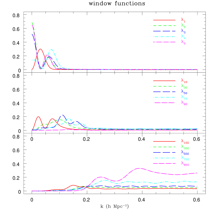
We performed the analysis described in Sec. 6 on these simulated catalogs. In Fig. 1 we show the window functions for selected moments calculated for a typical catalog in order of increasing eigenvalue, with the top plot showing the window functions for the moments with the five lowest eigenvalues, the middle showing five others associated with somewhat larger eigenvalues, and the bottom plot showing five more selected from the whole range of eigenvalues. This demonstrates that selecting moments that are least sensitive to small scales does in fact generally result in moments that are most sensitive to large scales; window functions of moments with larger eigenvalues are successively larger on nonlinear scales as expected. Thus the information contained in large eigenvalue moments comes mostly from scales where fluctuations are nonlinear and should not be included in a linear analysis.
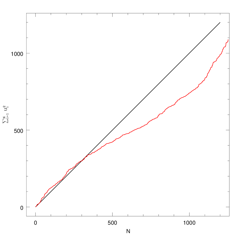
For our simulated catalogs, we know the “true” values of and . If we use these true values as our “guess” (see Sec. 6) to calculate the optimum moments, then the values of these moments calculated from the velocities should have unit variance, since the power spectrum model should be an excellent fit to the data. However, non–linear effects can cause higher order moments to deviate from unit variance. In Fig. 2 we show the sum of the first moments versus moment number for a typical catalog, where the moments are ranked in order of increasing eigenvalue. Note that for small , the sum tracks a line with unit slope, whereas for large the sum deviates from this line; this is an indication that the non–linear effects are causing the large moments to deviate from unit variance.
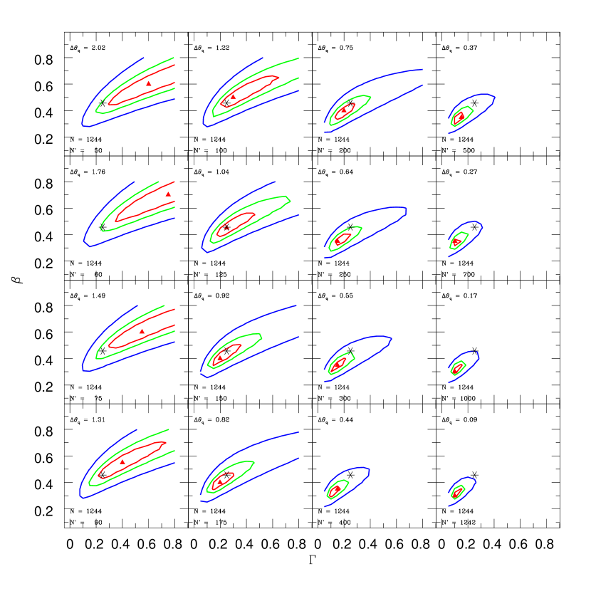
In Fig. 3 we show the results of the likelihood analysis on a typical catalog for different number of moments kept. For reference, we also give the value of for each as discussed in Sec. 4. Here the closed triangles correspond to the maximum likelihood values while the contours correspond to , , and of the maximum likelihood. The asterisk symbol corresponds to the input values used for the simulation, i.e. the “true” values for and . We see that in this case, inclusion of all of the information leads to the location of the maximum likelihood being skewed away from the true values (see the panel with ). However, when higher order moments are discarded, the location of the maximum likelihood corresponds well with the true values. For this particular catalog, with km/s, the criterion of Eq. (21) would give for the optimum number of moments to keep. The fact that the discarding of higher order moments leads to a much better agreement between the maximum likelihood location and the true values is a good indication that our analysis method is effectively removing small–scale, nonlinear velocity information.
Although the plots in Figs. 1–3 were calculated using a single catalog, we note that the results from other catalogs that we analyzed were not significantly different.
8 DISCUSSION AND CONCLUSIONS
In this paper we have presented a new method for the analysis of peculiar velocity surveys which removes contributions to velocities from small scale, nonlinear modes while retaining information about large scale motions. Our method selects a set of optimal moments constructed as linear combinations of velocities which are minimally sensitive to small scales. We have shown how the overall sensitivity of a set of moments to small scales can be quantified, and how to control this sensitivity through the choice of the number of moments to retain.
As discussed above, the necessity of assuming Gaussian statistics in our analysis raises the possibility that deviations from Gaussianity caused by the collapse of perturbations will interfere with the removal of small scale power and introduce additional unpredictable biases. While the results of Sec. 7 indicate that deviations from Gaussianity are not having a large effect, careful testing of our analysis method using simulated catalogs will be necessary to prove its effectiveness at filtering small–scale power. We are currently carrying out tests using catalogs drawn from simulations with a variety of parameter values, the results of which will be presented in a subsequent paper. This work will explore in more detail such issues as moment selection, optimal values for constants to be used in the analysis, and the dependence of the results of the analysis on whether the survey objects are galaxies or clusters of galaxies and how these objects are selected. We will also investigate differences in the small scale power present in simulations produced using , and tree codes. Once these tests are completed, we plan to apply our formalism to analyze existing velocity surveys, including the Mark III and SFI catalogs.
One of the merits of the formalism we have presented is its versatility; it can be applied to a wide variety of surveys with different geometries and densities. The formalism also allows for each object in the survey to have an independent velocity error. Versatility will be especially important as new distance measurement techniques begin to produce large surveys that may have a variety of characteristics. Our formalism will be particularly useful for surveys which use clusters of galaxies as tracers of the velocity field, which are necessarily quite sparse.
While we have focused on the use of our data compression formalism for the determination of power spectrum parameters through a likelihood analysis, it has broad applicability as a data filtering technique. Essentially, our formalism “rotates” the vector consisting of survey object velocities into a basis where the covariance matrix is diagonal with the new moments ranked as to their sensitivity to small scales. Discarding moments containing small scale information is equivalent to setting the value of these moments equal to zero; the vector of moments can then be rotated back to the survey object velocity basis. The result is essentially a “smoothed” or “linearized” velocity data set, which can be used as input for analysis methods that focus on large scale motions and assume linear theory. The amount and scale of the filtering can be adjusted by varying the constants and thresholds used in the construction of moments.
Finally, we note that the general technique we have developed for using data compression to filter out unwanted information may be useful in other areas of astrophysics; for example, in the analysis of cosmic microwave background data.
Appendix A APPENDIX
The line–of–sight velocity can be written in terms of the Fourier transform of the velocity field
| (A1) |
The covariance matrix then becomes
| (A2) | |||||
| (A3) | |||||
| (A4) | |||||
| (A5) |
where we have used the fact that and we have defined the tensor window function as the integral over the possible directions of the vector ,
| (A7) |
In linear theory, the velocity power spectrum is related to the density power spectrum by , with . This allows us to write as an integral over the density power spectrum,
| (A8) |
References
- Bardeen et al. (1986) Bardeen, J. M., Bond, J. R., Kaiser, N. & Szalay, A. S. 1986 ApJ 304 15
- Croft & Efstathiou (1994) Croft, R. & Efstathiou, G., 1994. Proceedings of the 11th Potsdam Cosmology Workshop : Large Scale Structure in the Universe, ed. Mücket., J. P. et al, World Scientific, astro–ph/9412024.
- da Costa et al. (1995) da Costa, L.N., Freudling, W., Wegner, G., Giovanelli, R., Haynes, M.P., & Salzer, J.J. 1996, ApJL, 468, L5
- Eldar (2000) Eldar, A. 2000, PhD Thesis
- Feldman & Watkins (1994) Feldman, H. A. & Watkins, R. 1994 ApJ 430 L17–20
- Feldman & Watkins (1998) Feldman, H. A. & Watkins, R. 1998 ApJ 494 L129–132
- Fisher (1935) Fisher, R. A. 1935, J. Roy. Stat. Soc., 98, 39
- Freudling et al. (1995) Freudling, W., da Costa, L. N., Wegner, G. Giovanelli, R., Haynes, M. P., & Salzer, J. J. 1995, AJ, 110, 2
- Hoffman & Zaroubi (2000) Hoffman, Y. & Zaroubi, S., 2000, ApJ 535 L5
- Hamilton (2000) 2000 MNRAS 312 257–284
- Hamilton & Tegmark (2000) 2000 MNRAS 312 285–294
- Jaffe & Kaiser (1995) Jaffe, A. & Kaiser, N. 1995 ApJ 255 26
- Kaiser (1988) Kaiser, N. 1988 MNRAS 231 149
- Kendall & Stuart (1969) Kendall, M. G. & Stuart, A. 1969 The advanced Theory of Statistics Vol. 2, London: Grifin.
- Kenney & Keeping (1954) Kenney, J.F., & Keeping, E.S. 1954, Mathematics of statistics, New York, Van Nostrand company 3rd ed.
- Klypin & Melott (1992) Klypin, A.A. & Melott, A.L. 1992 ApJ 399 397
- Lauer & Postman (1994) Lauer, T. & Postman, M. 1994 ApJ. 425 418–38
- Melott & Shandarin (1993) Melott, A. L. & Shandarin, S. F., 1993, ApJ 410 469–481
- Matsubara, Szalay & Landy (2000) Matsubara, T., Szalay, A.S. & Landy, S.D., 2000, ApJ 535:L1–L4
- Press et al. (1992) Press, W.H., Teukolsky, S.A., Vetterling, W.T. & Flannery, B.P., 1992 Numerical Recepies Cambridge University Press.
- Riess, Press & Kirshner (1995) Riess, A. G., Press, W. H., & Kirshner, R. P. 1995, ApJ, 438, L17
- Silberman et al. (2001) Silberman, L., Dekel, A., Eldar, A. & Zehavi, I., 2001, Submitted to ApJ , astro–ph/0101361
- Sodre & Lahav (1993) Sodre Jr., L. & Lahav, O. 1993, MNRAS, 260, 285
- Tegmark, Taylor & Heavens (1997) Tegmark, M., Taylor, A.N. & Heavens, A.F., 1997, ApJ 480 22–35
- Watkins & Feldman (1995) Watkins, R. & Feldman, H. A. 1995 ApJ 453 L73–76
- Watkins (1997) Watkins, R. 1997 MNRAS 292 L59