Effects of Heavy Elements and Excited States in the Equation of State of the Solar Interior

Abstract

Although 98% of the solar material consists of hydrogen and helium, the remaining chemical elements contribute in a discernible way to the thermodynamic quantities. An adequate treatment of the heavy elements and their excited states is important for solar models that are subject to the stringent requirements of helioseismology. The contribution of various heavy elements in a set of thermodynamic quantities has been examined. Characteristic features that can trace individual heavy elements in the adiabatic exponent $\gamma_{1}=(\partial\ln p/\partial\ln\varrho)_{s}$ (s being specific entropy), and hence in the adiabatic sound speed were searched. It has emerged that prominent signatures of individual elements exist, and that these effects are greatest in the ionization zones, typically located near the bottom of the convection zone. The main result is that part of the features found here depend strongly both on the given species (atom or ion) and its detailed internal partition function, whereas other features only depend on the presence of the species itself, not on details such as the internal partition function. The latter features are obviously well suited for a helioseismic abundance determination, while the former features present a unique opportunity to use the sun as a laboratory to test the validity of physical theories of partial ionization in a relatively dense and hot plasma. This domain of plasma physics has so far no competition from terrestrial laboratories. Another, quite general, finding of this work is that the inclusion of a relatively large number of heavy elements has a tendency to smear out individual features. This affects both the features that determine the abundance of elements and the ones that identify physical effects. This property alleviates the task of solar modelers, because it helps to construct a good working equation of state which is relatively free of the uncertainties from basic physics. By the same token, it makes more difficult the reverse task, which is constraining physical theories with the help of solar data.

1 Introduction

The equation of state is one of the most important ingredients in solar and stellar modeling. Assessing the quality of the equation of state is not easy, though. Because of the relevant high temperatures and densities, there are no sufficiently accurate laboratory measurements of thermodynamic properties that could assist the solar modeler. However, the observational quality of helioseismology has become so high that high-precision thermodynamic quantities must be part of state-of-the-art solar models. So, strictly speaking, at the moment only theoretical studies of the equation of state can be pursued. But this is a too pessimistic view. Helioseismology puts significant constraints on the thermodynamic quantities and has already delivered powerful tools to test the validity and accuracy of theoretical models of the thermodynamics of hot and dense plasmas (Christensen-Dalsgaard and Däppen, 1992; Christensen-Dalsgaard et al., 1996).

There are two important reasons why the thermodynamics can be tested with solar data. First, the accurate solar oscillation frequencies obtained from space and ground-based networks observation have led to a much better understanding of the solar interior with a very high level of accuracy. Second, thanks to the existence of the solar convection zone, the effect of the equation of state can be disentangled from the other two important input-physics ingredients of solar models, opacity and nuclear reaction rates. This simplification is due to the fact that in large parts of the convection zone, the convective motion is very close to adiabatic, which leads to a stratification that is equally very close to adiabatic. Thus, except in the small superadiabatic zone close to the surface, the uncertainty arising from our ignorance of the details of the convective motion does not matter. As a consequence, inversions for the thermodynamic quantities of the deeper layers of the convection zone promise to be sensitive to the small non-ideal effects employed in different treatments of the equation of state (Christensen-Dalsgaard et al., 1996; Nayfonov and Däppen, 1998).

Before the 1980s, simple models of the equation of state were used in solar modeling. Their physics was based on the one hand on ionization processes modeled by the Saha equation and on the other hand on electron degeneracy. Fairly good results had been obtained in this way, for instance, by the equation of state of Eggleton, Faulkner and Flannery (1973). However, it turned out soon that the observational progress of helioseismology had reached such levels of accuracy that further small non-ideal terms in the equation of state became observable. Inclusion of a (negative) Coulomb pressure correction became imperative (Ulrich, 1982; Shibahashi, Noels and Gabriel, 1983; Christensen-Dalsgaard, Däppen and Lebreton, 1988). With this Coulomb correction being the main non-ideal term, the subsequent upgrade of the EFF formalism to include the Coulomb term became quite successful; its realization is the so-called CEFF equation of state (Christensen-Dalsgaard and Däppen, 1992). Since then, other non-ideal effects, such as pressure ionization and detailed internal partition functions of bound states were also considered. Examples of such more advanced equation of state are the MHD equation of state (Hummer and Mihalas, 1988; Mihalas, Däppen and Hummer, 1988; Däppen, Mihalas and Hummer, 1988) and the OPAL equation of state (Rogers, Swenson and Iglesias, 1996), as well as the SIREFF and its sibling, the EOS-1 equation of state (Guzik and Swenson, 1997; Irwin et al., 2001). These efforts in basic physics have paid off well, because a significantly better agreement between theoretical models and observational data has been achieved when using such improved equations of state (Christensen-Dalsgaard et al., 1996; Basu, Däppen and Nayfonov, 1999).

Despite this progress, the theoretical models are not yet sufficient (see section 3.4). And it turns out that complicated many-body calculations are necessary even if the solar plasma is only slightly non-ideal. In recent efforts for a better equation of state, realistic microfield distributions (Nayfonov et al., 1999) and relativistic electrons (Elliot and Kosovichev, 1998; Gong and Däppen, 2000; Gong, Däppen and Zejda, 2001) have been introduced in solar models, but even these most refined solar models have discrepancies with respect to the observed solar structure that are much larger than the observational errors themselves. Therefore, further investigations are still necessary. We note in passing that while the aforementioned non-ideal theories have all at least some theoretical footing, sometimes pure ad-hoc formalisms can mimic reality even better; an example is the recent pressure-ionization parameterization of Baturin et al. (2000).

The thermodynamic quantities of solar plasma do not only depend on temperature and density, but also on the characteristic properties of all atoms, ions, molecules, nuclei and electrons. A major complication is that the chemical composition changes through the lifetime of the sun. Abundance changes are a consequence of the several major mixing processes that have been considered in solar models (Kippenhahn and Weigert, 1990). Another change is caused by the nuclear reactions in the solar center, which convert four hydrogen atoms into one helium atom, and produce, as by-products, several other species, such as ³He, carbon, nitrogen and oxygen, during the p-p and CNO chain reactions. And finally, even in the solar convective zone the composition can change in time. Although at any given moment, all elements should be homogeneously distributed, due to the thorough stirring of the convective motion on a very short time scale (on the order of a month and less), over longer time scales, the chemical composition can change nonetheless. The major effect is the so-called gravitational settling, which involves the depletion of heavier species in the stable layers immediately below the convection zone. This depletion is then propagated upward into the convection zone by convective overshoot that dips into the depleted regions. Since the 1990s, helioseismology has been successfully put constraints on solar models with various kinds of mixing (Cox, Guzik and Kidman, 1989; Michaud and Vauclair, 1991; Bahcall and Pinsonneault, 1992; Proffitt, 1994; Thoul, Bahcall and Loeb, 1994; Richard et al., 1996; Brun, Turck-Chièze and Zahn, 1999), but it is clear that a new, thermodynamics-based determination of the local abundance of heavy elements inside the sun would deliver a powerful additional constraint.

In a first part, this paper consists of a systematic study of the contribution of various heavy elements in a representative set of thermodynamic quantities. Intuitively, one might think that unlike in the opacity, in the equation of state, the influence of details in the heavy elements is not as critical, because the leading ideal-gas effect of the heavy elements is proportional to their total particle number. Their influence should therefore be severely limited, since all heavy elements together only contribute to about 2% in mass. However, as shown in Baturin et al. (2000) and in section 3.4, helioseismology has become so accurate that even details of the contribution of heavy elements beyond the leading ideal-gas term are in principle observable. In a further part of this paper, we show that one the one hand, there are element-dependent, but physics-independent, features of the heavy elements. This result has promising diagnostic possibilities for the helioseismic heavy-element abundance determination. On the other hand, we have also found features in the same thermodynamical quantities which do depend on the detailed physical formalism for the individual particles. Such features will lend to a diagnosis of the physical foundation of the equation of state.

2 Synopsis of equation-of-state issues

There are two basic approaches: the so-called chemical and physical pictures. In the chemical picture, one assumes that the notion of atoms and ions still makes sense, that is, ionization and recombination is treated like a chemical reaction. One of the more recent realizations of an equation of state in the physical picture is the MHD equation of state. It is based on the minimization of a model free energy. The free energy models the modifications of atomic states by the surrounding plasma in a heuristic and intuitive way, using occupation probabilities. The resulting internal partition functions $Z_{s}^{\rm int}$ of species $s$ in MHD are

$$Z_{s}^{\rm int}=\sum_{i}w_{is}\,g_{is}\,\exp[-(E_{is}-E_{1s})/(k_{\rm{B}}T)]\ ,$$ (1)

Here, $is$ label states $i$ of species $s$. $E_{is}$ are their energies, and the coefficients $w_{is}$ are the occupation probabilities that take into account charged and neutral surrounding particles. In physical terms, $w_{is}$ gives the fraction of all particles of species $s$ that can exist in state $i$ with an electron bound to the atom or ion, and $1-w_{is}$ gives the fraction of those that are so heavily perturbed by nearby neighbors that their states are effectively destroyed. Perturbations by neutral particles are based on an excluded-volume treatment and perturbations by charges are calculated from a fit to a quantum-mechanical Stark-ionization theory. Hummer & Mihalas’s (1988) choice had been

$$\ln w_{is}=-\Big{(}\frac{4\pi}{3V}\Big{)}\left\{{\sum_{\nu}}N_{\nu}(r_{is}+r_{1\nu})^{3}+16\left[\frac{(Z_{s}+1)e^{2}}{\chi_{is}k_{is}^{1/2}}\right]^{3}\sum_{\alpha\neq e}N_{\alpha}Z_{\alpha}^{3/2}\right\}\ ,$$ (2)

Here, the index $\nu$ runs over neutral particles, the index $\alpha$ runs over charged ions (except electrons), $r_{is}$ is the radius assigned to a particle in state $i$ of species $s$, $\chi_{is}$ is the (positive) binding energy of such a particle, $k_{is}$ is a quantum-mechanical correction, and $Z_{s}$ is the net charge of a particle of species $s$. Note that $\ln w_{is}\propto\ -n^{6}$ for large principal quantum numbers $n$ (of state $i$), and hence provides a density-dependent cut-off for $Z_{s}^{\rm int}$.

The physical picture provides a systematic method to include nonideal effects. An example is the OPAL equation of state, which starts out from the grand canonical ensemble of a system of the basic constituents (electrons and nuclei), interacting through the Coulomb potential. Configurations corresponding to bound combinations of electrons and nuclei, such as ions, atoms, and molecules, arise in this ensemble naturally as terms in cluster expansions. Effects of the plasma environment on the internal states, such as pressure ionization, are obtained directly from statistical-mechanical analysis, rather than by assertion as in the chemical picture.

Although the stellar plasma we deal with is assumed to be electrically neutral in a large volume, it is a mixture of charged ions and electrons inside. The Coulomb force between these charged particles is long range. By doing the first order approximation, the so-called Debye and Hückel (1923) potential results. It is the approximation of the static-screen Coulomb potential (SSCP), which describes the interaction between charged particles as

$$\psi(r)=Ze\,\frac{\rm{e}^{-r/\lambda_{\rm{D}}}}{r}\ ,$$ (3)

where $Z$ is the net charge of the particle, $e$ is electron charge, $r$ is the distance to the center of the target particle, and $\lambda_{\rm{D}}$ is the Debye length. The corresponding free-energy, which is sometimes called the Debye-Hückel free energy, can then be obtained. It has become widely used (Graboske, Harwood and Rogers, 1969; Mihalas, Däppen and Hummer, 1988). Furthermore, in order to eliminate the short-range divergence in the Debye-Hückel potential, a cutoff function

$$\tau(x)=3x^{-3}\,[\ln(1+x)-x+\frac{1}{2}x^{2}]=3x^{-3}\,\int_{0}^{x}\frac{y^{2}}{1+y}\rm{d}y\ ,$$ (4)

was introduced, where $x=r_{\min}/\lambda_{\rm{D}}$, with $r_{\min}$ being the distance of closest approach (the minimum distance that the center of two particles can reach). This factor $\tau$ is essential to get rid of the possibility of a negative total pressure when density of the plasma is becoming high. However, it has become known for some time (Baturin et al., 1995; Däppen, 1996) that this $\tau$ factor (Eq. 4) can produce some unforeseen and unjustified effects on some thermodynamic quantities in solar equation of state, which we will discuss in more detail in Sect. 4. In order to clearly disentangle the effects of the heavy elements and those of the $\tau$ factor, in this paper we are using the MHD and CEFF equations of state with a Debye-Hückel theory but without a $\tau$ correction unless explicitly stated.

In helioseismic inversions for equation-of-state effects, the resulting natural second-order thermodynamic quantity is the adiabatic gradient (Basu and Christensen-Dalsgaard, 1997), which is itself closely related to adiabatic sound speed, which can also be the result of inversions. Such inversions are called “primary”. However, in the diagnosis of physical effects, other second-order thermodynamic quantities can in principle be more revealing than the adiabatic gradient (Nayfonov and Däppen, 1998). Unfortunately, the helioseismic inversion for these other thermodynamic quantities is less direct, because additional physical assumptions must be made. Such inversions are therefore called “secondary”. In view of future primary and secondary inversions, we study here not only the adiabatic gradient, but more systematically the complete set of the following three second-order thermodynamic quantities

$$\chi_{\rho}=(\partial\ln p/\partial\ln\rho)_{T}\ ,$$ (5)

$$\chi_{T}=(\partial\ln p/\partial\ln T)_{\rho}\ ,$$ (6)

$$\gamma_{1}=(\partial\ln p/\partial\ln\rho)_{s}\ ,$$ (7)

where $p$ is pressure, $\rho$ is density, $T$ is temperature, and $s$ is specific entropy. All other second-order quantities can be derived as functions of these three quantities.

3 Effects of heavy elements

3.1 Difference between selected equations of state

It is well known that the heavy-element abundance of stars is crucial for opacity, where a certain single heavy element often leads to the dominant contribution. However, one would expects a much less dramatic effect in the equation of state. Quantitatively, in the sun, the abundance of heavy-elements is small (about 2 percent in mass) and their influence in the equation of state is roughly proportional to their number abundance, which is about an order of magnitude smaller. Nevertheless, helioseismology has already revealed heavy-element effects (Däppen et al., 1993; Baturin et al., 2000).

In this paper, we study the effect of the heavy elements with the help of the MHD equation of state. We choose the MHD equation of state, because it contains relatively detailed physics, has been widely used in solar modeling (thus giving a benchmark for our analysis), and most importantly, because among all the non-trivial equations of state it is the only one with which a systematic study of the influence of individual elements and their detailed physical treatment can be carried out. The other non-trivial equations of state are only available in pre-computed tabular form, with fixed heavy-element abundance.

The physical conditions for which the different equations of state have been calculated are from a solar model [model S of Christensen-Dalsgaard et al. (1996)], restricted to the convection zone, that is, the range relevant for a helioseismological equation-of-state diagnosis. For our conceptual and qualitative study we do not need the most up-to-date values for the chemical composition. Thus, for simplicity, we have chosen a typical chemical composition of mass fractions $X=0.70$, $Y=0.28$ and $Z=0.02$. Since we are also comparing our result with the OPAL equation of state [which is so far best for solar models (Christensen-Dalsgaard et al., 1996)], for the sake of consistency, we have chosen a distribution of heavy elements in exactly the same way as in the OPAL tables (Rogers, Swenson and Iglesias, 1996). For convenience, we here list this choice in Table 1.

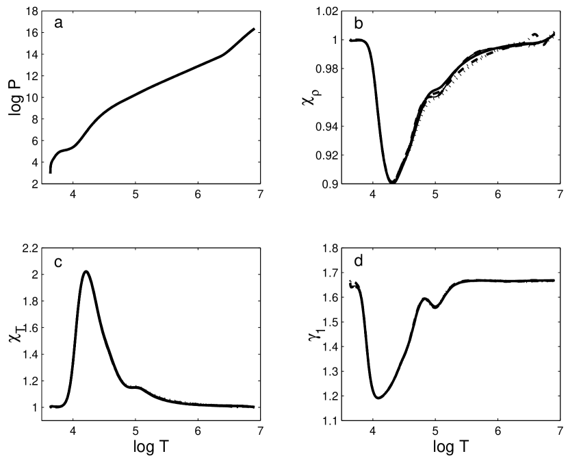
Figure 1: Absolute values of thermodynamic quantities for different equations of state with a regular 6-element mixture (Rogers, Swenson and Iglesias, 1996) for conditions of the solar convection zone. Dashed line: MHD; Thick Solid line: OPAL; Dashed-dotted line: CEFF; Dotted line: SIREFF; Thin Solid line: MHD_GS.

In Figs. 1 and 2 we show pressure, $\chi_{\rho}$, $\chi_{T}$ and $\gamma_{1}$ in a solar model with the 6-element mixture of Table 1 for several popularly used equations of state. Both absolute values, and for finer details, relative differences with respect to the MHD equation of state are displayed. The equations of state are:
MHD - standard MHD with the usual occupation probabilities (Hummer and Mihalas, 1988).
MHD_GS - standard MHD but with internal partition functions of heavy element truncated to the ground state term (however, the internal partition function of H and He are not truncated, which is different from Nayfonov and Däppen (1998) [ND98 hereafter] and the H-He mixture models of section 4).
OPAL - interpolated from the OPAL tables (Rogers, Swenson and Iglesias, 1996) [except for the H-He-C mixture models, which were directly calculated by one of us (AN)].
CEFF - Christensen-Dalsgaard and Däppen (1992)
SIREFF - Guzik and Swenson (1997)
As found by ND98, for a pure hydrogen and a hydrogen-helium mixture under solar conditions, among the possible thermodynamic quantities (that derive from the second derivatives of the free energy), it is the quantity $\chi_{\rho}$ [Fig. 1 (b)] which reveals most physical effects, and this already in the absolute values. Of course, other thermodynamic quantities contain signatures of the same physical effects as well, but often they would show up only in the de-facto amplification of relative differences. The sensitivity of $\chi_{\rho}$ is mainly due to the fact that in ionization zones it varies considerably less than the other thermodynamic quantities. Finer effects are therefore overlaid on a smaller global variation and show therefore up already in the absolute plots. Specifically, the main result of ND98 was a “wiggle” in $\chi_{\rho}$, resulting from the density dependent occupation probabilities for the excited states of hydrogen in MHD.

Our study deals with the combined effect of several different heavy elements and, importantly, several different physical mechanisms that describe the interaction between the ground and excited states of their atoms and ions with the surrounding plasma. In order to disentangle effects from individual elements, we have studied the heavy-element effects separately for each element. Before we interpret the heavy-element features in Fig. 1, first we should like to mention an effect not related to heavy elements, which nonetheless demonstrates the power of our analysis. Fig. 1 (d) shows, at very low temperature ($\log T\leq 3.5$), a feature. For instance, in $\gamma_{1}$ a dip appears in most equations of state except in CEFF. It is obviously the signature of H₂ molecular dissociation (Lebreton and Däppen, 1988), a process not included in the CEFF equation of state.

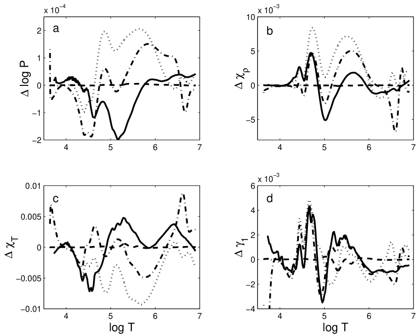
Figure 2: Relative difference in thermodynamic quantities of Fig. 1 in the sense [(X - X_MHD)/ X_MHD]. Dashed line: MHD; Solid line: OPAL; Dashed-dotted line: CEFF; Dotted line: SIREFF.

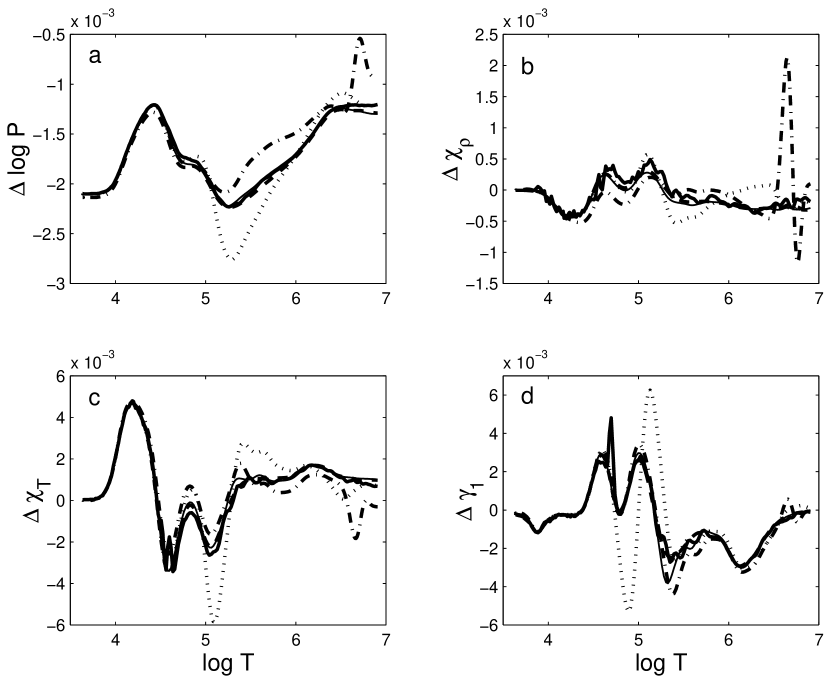
Figure 3: Difference in thermodynamic quantities between the 6-element mixture and the hydrogen-helium mixture for various equations of state. Difference are in the sense [X(Model)_6-element - X(Model)_H-He]. Line styles the same as in Fig. 1.

Next, we have compared the contribution of heavy elements in the various equations of state (Fig. 3). For each particular equation of state, we have computed the relative difference between the regular 6-element mixture and a hydrogen-helium mixture (mass fractions being $X=0.70$, $Y=0.30$). This difference is much smaller than the one given in Fig. 2, suggesting that the biggest difference among different models of equation of state is related to the treatment of hydrogen and helium. However, as shown below, this does not mean that for second-order thermodynamic quantities in solar models of helioseismic precision the contribution of heavy elements would be negligible (see section 3.4).

3.2 Signature of individual heavy elements

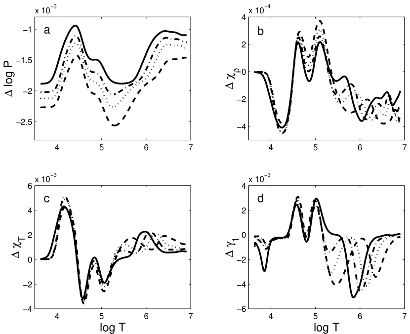
Figure 4: Difference in thermodynamic quantities between the hydrogen-helium-and-one-heavy-element mixture and the hydrogen-helium mixture for the MHD equation of state. Differences are in the sense [X_H-He-Z - X_H-He]. Solid line: H-He-C; Dashed-dotted line: H-He-N; Dotted line: H-He-O; Dashed line: H-He-Ne.

In order to reveal the contribution of each individual heavy element, we have calculated solar models with particular mixtures. In each case, hydrogen and helium abundances were fixed with mass fractions $X=0.70$ and $Y=0.28$; the remaining 2% heavy-element contribution was topped off by only one element, carbon, nitrogen, oxygen and neon, respectively. We have then compared these models with the hydrogen-helium mixture model in Fig. 4 (this mixture is obtained by filling the two percent reserved for heavy elements with additional helium). The expectation is that the biggest deviations between these special models, and the one with the complete heavy-element mixture, will result (i) from the change in the total number of particles per unit volume and (ii) from the different ionization potentials of the respective elements. Because the solar plasma is only slightly non-ideal, the leading pressure term is given by the ideal-gas equation

$$pV=Nk_{B}T\ ,$$ (8)

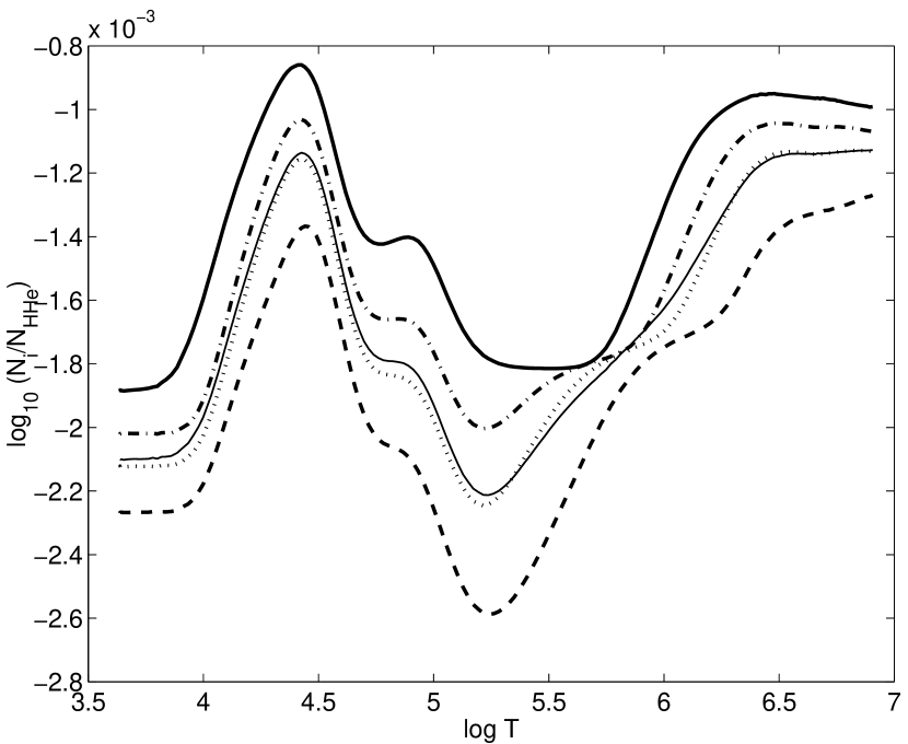
Figure 5: Difference in the total number of particles between the hydrogen-helium-and-one-heavy-element mixture and the hydrogen-helium mixture for the MHD equation of state. Differences are in the sense [N_H-He-Z - N_H-He]. Thin Solid line: 6-element mixture; otherwise the same as in Fig. (4).

with $p$ standing for pressure, $N$ the number of particles, and $k_{B}$ the Boltzmann constant. Because of their higher mass, the number of heavy-element atoms is obviously smaller than that of helium atoms representing the same mass fraction. However, against this reduction in total number there is an offset due to the ionization of their larger number of electrons which becomes stronger at higher temperatures. The net change of the total number of particles is therefore a combination of these two effects. In Fig. 5 we show the difference between the total number of particles in these models, and we see that indeed it explains the difference in total pressure well.

Since the second-order thermodynamic quantities (Eq. 5-7) [see Fig. 4 (b-d)] are independent of the total number of particles, they can reveal signatures of the internal structure of each element more directly. Therefore, at low temperatures ($\log T<5.2$), the difference with respect to a hydrogen-helium mixture plasma is similar for all the heavy elements, because the difference in the second-order quantities mainly comes from the fact that the 2% helium in the H-He mixture are already partly ionized, while the replacing heavier elements are still mainly neutral. However, as temperature rises, a signature of the ionization of the individual heavy element appears. This selective modulation of second-order thermodynamic quantities, as well as another property discussed further below, allow us in principle to identify single heavy elements in the solar convection zone, in analogy to optical spectroscopy.

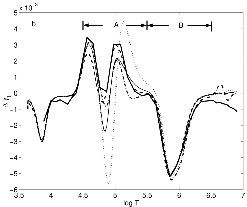
Figure 6: Difference in thermodynamic quantities between the H-He-C mixture and the H-He mixture for various equations of state. Differences are in the sense [X(Model)_H-He-C - X(Model)_H-He]. Line styles the same as in Fig. (1).

Our next comparison has the purpose to disentangle even further the contribution of the mere presence of each heavy element from the more subtle influence of different physical formalisms. In Fig. 6 the H-He-C models (with mass fractions 0.70:0.28:0.02) are compared with the H-He models (0.70:0.30) for our set of different equations of state. This procedure eliminates most of the difference due to the treatment of hydrogen and helium in each individual equation of state and therefore isolates the behavior of carbon in each of our equations of state. We note that here, roughness appears in the OPAL equation of state, because the sensitivity of our analysis has almost reached the reasonable limit of accuracy that can be obtained by interpolation in the OPAL tables.

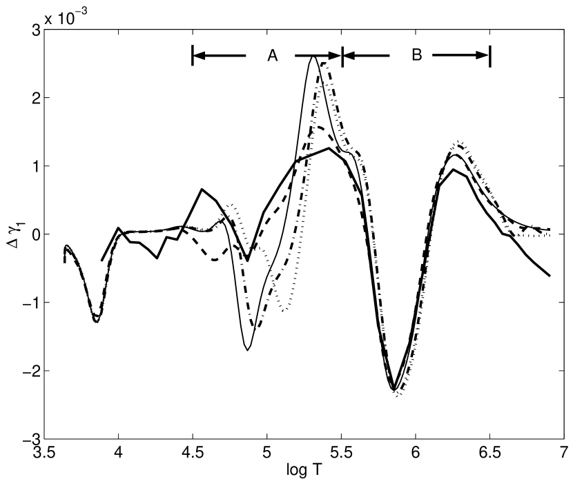
Figure 7: Difference in thermodynamic quantities between the 6-element mixture and the H-He-C mixture for various equations of state. Differences are in the sense [X(Model)_6-mixture - X(Model)_H-He-C]. Line styles the same as in Fig. (1).

From Fig. 6 (a), we can see that among the thermodynamic quantities, $\Delta\chi_{T}$ reveals the biggest differences between the equations of state in the temperature range of $4.5<\log T<5.5$ (named region “A” in the figure). Common features can be identified when $\log T>5.5$ and $\log T<4.5$. Such features are also visible in the $\Delta\gamma_{1}$ graph between H-He-C and H-He shown in Fig. 6 (b), and between H-He-C and the regular 6-element mixture shown in Fig. 7.

In the region “A” of Fig. 7 the MHD and OPAL results together differ significantly from the other three formalisms; they appear closer to the reference 6-element mixture model than to the other models. One obvious reason is that neither MHD_GS nor CEFF nor SIREFF include excited states of heavy elements (in this figure carbon), while both MHD and OPAL do, although OPAL does it quite differently (Rogers, 1986). Our figure would then suggest that the difference between MHD and OPAL on the one hand, and the other three formalisms on the other hand, appears most likely due to the contribution of the excited states of carbon. In addition, it also appears that that it matters less that excited states are treated differently than that they are not neglected. It will be a challenge for helioseismology to distinguish between such small differences.

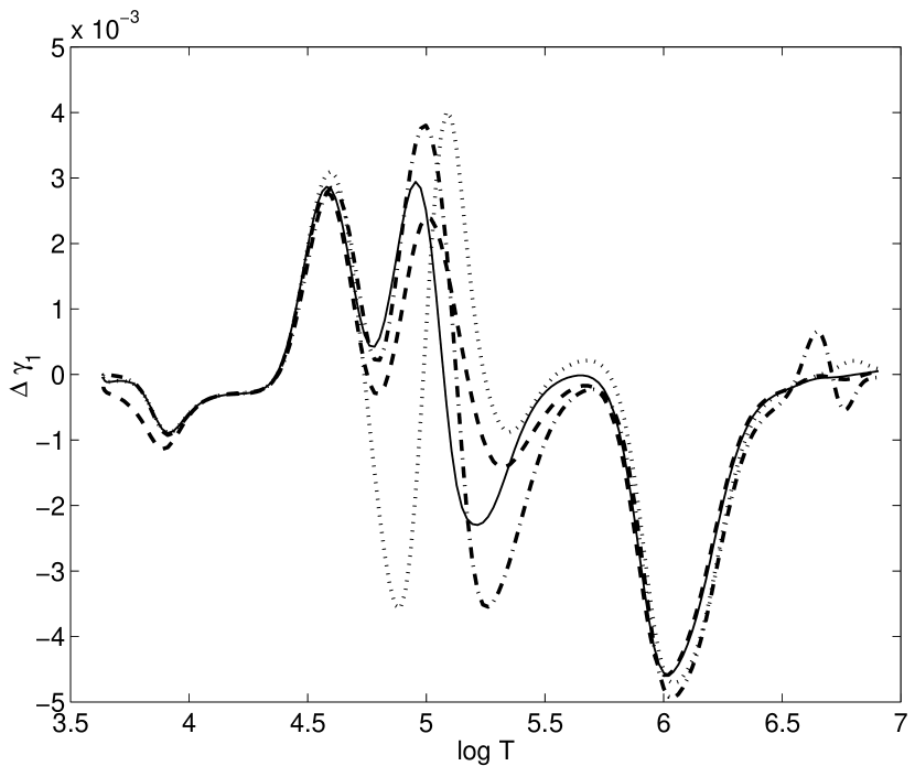
Figure 8: Difference in thermodynamic quantities between the H-He-N mixture and the H-He mixture for some models of equation of state. Differences are in the sense [X(Model)_H-He-N - X(Model)_H-He]. Line styles the same as in Fig. (1).

The bump in $\Delta\gamma_{1}$ in the region “B” of either Fig. 6 (b) or Fig. 7 is totally independent of the equation of state used. By comparing with Fig. 4 (d), it follows that the feature is likely due to the ionization of carbon at that temperature in general, quite independent of details in the equation of state. The strength and robustness of this profile and its relative independence on the equation of state qualify it ideally for a helioseismic heavy-element abundance determination. This is true because the profile does not only appear for carbon, but also for all other heavy elements which exhibit a similar feature independent of the equation of state. As an example, the analogous phenomenon for nitrogen at its higher ionization temperature is revealed by the H-He-N model in Fig. 8. It is clear from Fig. 4 (d) that each heavy element has its own profile, and in analogy to the helioseismic helium-abundance determination (Vorontsov et al., 1994; Baturin et al., 2000), these profiles promise to be used in future inversions of solar oscillation frequencies to determine the abundance of the heavy-elements.

3.3 Effects of the number of heavy elements in the equation of state

Another important issue in the study of heavy-element effects in the solar equation of state is how many elements should be considered, that is, what is the error if not enough elements are included. We address this question by adding species one by one until we reach the 15 element mix considered in the original MHD equation of state (Mihalas et al., 1990) to see if there is subset that is adequate for helioseismic accuracy. To be more specific, we have again set the total abundance of all heavy elements to be fixed at $Z=0.02$, but this time we follow the Grevesse and Sauval (1998) abundance, which slightly differs from the simplified values of Table 1. We label the mixtures by the number of species including H and He (thus a 3-element mixture means H-He-C; a 4-element H-He-C-N, etc.). To reconcile the absolute mass fractions of the Grevesse and Sauval (1998) mixture with our specification of a fixed mass fraction $Z=0.02$, some form of topping off is necessary. In the case of the first 6 elements, we have chosen to readjust the last element to top off to $Z=0.02$, with the other heavy elements being set to the Grevesse and Sauval (1998) abundance. The same convention holds for the 7th element, which is iron. However, from this case onward to the full 15-element mixture, we have always used iron to top off to $Z=0.02$, with the other heavy elements always having their Grevesse and Sauval (1998) abundance.

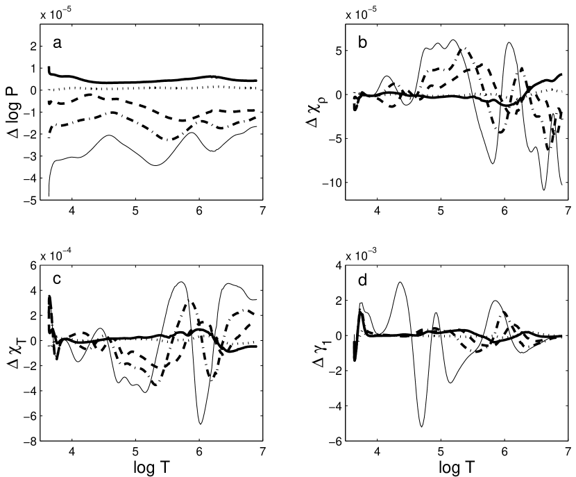
Figure 9: Relative difference of thermodynamic quantities between a sequence of reduced mixtures and the full 15-element mixture for the MHD equation of state. Differences are in the sense (X - X_15-element)/X_15-element. In panels (a-c): Thin Solid line: 4-element; Dashed-dotted Line: 5-element; Dashed Line: 6-element; Thick Solid Line: 7-element; Dotted Line: 11-element. In panel (d): Thin Solid line: 3-element; Dashed-dotted Line: 4-element; Dashed Line: 5-element; Thick Solid Line: 6-element; Dotted Line: 7-element.

The results of this systematic procedure to add heavy elements one by one are shown in Fig. 9. We distinguish two cases. First, regarding pressure, the larger the number of heavy elements considered is, the closer pressure approaches that of the full mixture. This is easy to understand from the role of the effect of individual heavy elements discussed in Sec. 3.1. Second, and more interesting, regarding the second-order thermodynamic quantities, the larger the number of heavy elements considered is, the smoother the curves overall become. The reason is that when more species are included the less weight each individual species obtains and thus its contribution with its specific features becomes reduced. In addition, different species have their own profile which sometimes leads to partial cancellations. Overall, then, the effect of a mixture with a larger number of heavy elements is manifested by the relatively flat profiles of Fig. 9 (b-d). Third, regarding the minimum number of heavy elements necessary for accurate helioseismic studies, we conclude that the inclusion of new species of heavy elements becomes less and less critical if at least ten of the most abundant species are included. Inclusion of more elements will lead to such small differences in the equation of state that they appear to be undetectable by current helioseismological studies (see the following section). Fourth, however, the currently popular 6-element mixture used in OPAL is still inadequate in as far as it leads to a deviation with respect to the full mixture, attaining up to $3\times 10^{-4}$ in $\gamma_{1}$ at the base on solar convection zone. And since the OPAL data are so far only available in tabular form, the inevitable interpolation error, which is typically of the same order, only aggravates this situation.

3.4 Current resolution power of helioseismology

The observational resolution of helioseismic inversions is demonstrated in Fig. 10. It shows the result of an inversion (Basu, Däppen and Nayfonov, 1999) for the intrinsic $\gamma_{1}$ difference between the sun and a solar model (Basu and Christensen-Dalsgaard, 1997). The intrinsic difference is the part of the $\gamma_{1}$ difference due to the difference in the equation of state itself [and not the additional part implied by the change in solar model due to that of the equation of state, which induces a further $\gamma_{1}$ difference (Basu and Christensen-Dalsgaard, 1997)]. The main result of Fig. 10 is that present-day helioseismology has reached an accuracy of almost $10^{-4}$ for $\gamma_{1}$. The effects discussed in this paper are therefore within reach of observational diagnosis.

More specifically, studies such as the one shown in Fig. 10 reveal the influence of the equation of state by an analysis of the difference between the solar values obtained from inversions and the ones computed in reference models (standard solar models). In the case of Fig. 10, two sets of reference models are compared to the solar data, one set based on the MHD equation of state, the other set on OPAL. Because of the differential nature of these inversions, they become more reliable when the reference model is close to the real solar structure. In the last years, the solar models were significantly improved, thanks to the constraints of helioseismology. In particular, diffusion has now become part of the standard solar model (Christensen-Dalsgaard et al., 1996) and it was included in the calibrated reference models of Basu, Däppen and Nayfonov (1999) (models M1–M8 of Table 2). Their composition profiles (in particular the surface helium abundance $Y_{\rm s}$) were those obtained from helioseismological inversions by Antia and Chitre (1998). All models had $Z/X=0.0245$ (Grevesse and Noels, 1993). In the inversions, Basu, Däppen and Nayfonov (1999) tested the robustness of the inferred results against uncertainties in the solar-model inputs using a number of different solar models (see their paper for details of the tests made). All of the models M1–M8 had either the MHD or the OPAL equation of state, and they were all using OPAL opacities (Iglesias and Rogers, 1996), supplemented by the low temperature opacities of Kurucz (1991). Since one of the most uncertain aspects of solar modeling is always the formulation of the convective flux, two different formalisms were used – standard mixing length theory (MLT) and the Canuto and Mazitelli (1991) formalism (CM). The two formalisms give fairly different stratifications in the outer regions of the sun. Fig. 10 clearly shows that helioseismology has the potential to address the small effects from heavy elements such as discussed in Fig. 7 and Fig. 8.

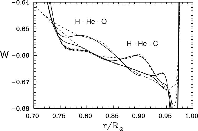
Figure 11: The quantity W=$({\rm d}c^{2}/{\rm d}r)/g(r)$ obtained from an inversion of solar p-mode frequencies and three solar models with different heavy-element abundances (Baturin et al., 2000). The observational curve is marked with vertical bars (estimated inversion error). The pair of solid and dashed lines that follows the observational $W$ most closely is from a model with the usual solar composition (dashed line: $W$ computed directly from the solar model; solid line: result of the same inversion procedure as for the observational curve, but with artificial mode frequencies from the solar model). The two other pairs of solid and dashed lines (“H-He-C” and “H-He-O”) are from models with a heavy-element composition of pure carbon and oxygen, respectively, of an amount equal to the total solar heavy-element abundance. Solid and dashed lines have the same meaning as before. In contrast to Fig. 10, the inversions here are absolute (that is, not relative to a reference model). All models in this figure include electrostatic screening (Eq. 3).

While Fig. 10 is based on numerical inversions, asymptotic inversion techniques can shed light from a different angle. In particular, they are well suited for heavy-element abundance determinations, as demonstrated by Fig. 11 from Baturin et al. (2000). Fig. 11 shows the result of an asymptotic inversion introduced by Gough (1984) for the helioseismic helium abundance determination. The inversion is for the so-called quantity $W$, which is a function of solar structure

$$W={{\rm d}c^{2}\over{\rm d}r}{1\over g(r)}\ .$$ (9)

Here, $g(r)$ is the local gravitational acceleration at position $r$ in the sun. The quantity $W$ is useful because of its equality with a purely thermodynamic quantity if the stratification is assumed to be perfectly adiabatic (otherwise, the equality is violated by the amount of the non-adiabaticity). For adiabatic stratification, the following relation holds (Gough, 1984)

$$W={1-{\gamma_{1}}-{\gamma}_{1,\rho}\over 1-{\gamma}_{1,c^{2}}}\ ,$$ (10)

with the derivatives

$$\gamma_{1,\rho}=\left({\partial\ln\gamma_{1}\over\partial\ln\rho}\right)_{c^{2}},\gamma_{1,c^{2}}=\left({\partial\ln\gamma_{1}\over\partial\ln c^{2}}\right)_{\rho}\ .$$ (11)

While the reader is referred to (Baturin et al., 2000) for more detail, here we merely mention that similarly to Fig. 10, Fig. 11 shows $W$ in the sun and in two artificial solar models, but in contrast to Fig. 10, the inversions of Fig. 11 are absolute and not relative to a reference model. The comparison models of Fig. 11 are based on the H-He-C composition of section 3.2 (where pure carbon is representing the total heavy-element abundance), and the analogous H-He-O composition, respectively. It is no surprise that since the quantity $W$ involves derivatives of $\gamma_{1}$, it is even more sensitive to equation-of-state effects than $\gamma_{1}$ itself. That this is indeed the case is clearly reflected in Fig. 11, where the two models, which are, after all, very close to each other, lead to values of $W$ which differ by an amount far larger than the accuracy of the inversion (indicated by error bars). Since the models of Fig. 11 exhibit exactly the same variation of the heavy-element composition as the models of the present paper, it is clear that Fig. 11 has convincingly demonstrated that the effects found and studied here are already well within the reach of present-day observational accuracy.

4 Discussion

4.1 Role of the occupation probability of the ground state

As we have mentioned in section 1, the effect of the treatment of excited states of atomic and ionic species can show up under certain circumstances. ND98 pointed out that the existence of the wiggle in the $\chi_{\rho}$ diagram in the MHD equation of state [see Fig. 1 (b)] is a genuine effect of neutral hydrogen even if it occurs in a region where most of hydrogen is already ionized. The wiggle is caused by the specific form of the density-dependent occupation probabilities of excited states in MHD. However, ND98, did not examine the influence of the ground state. Thus, to see if the excited states do, or do not, behave in the same way as the ground states, we have carried out a numerical experiment in which we have switched on and off the MHD-type occupation probabilities [see Eq. (2) for definition] of all ground states of all species. To switch off the MHD-type occupation probability of a ground state, we have simply set $w_{1s}=1$, where $s$ stands for a given species (atom or ion of an element), with all of the other $w_{is}$ remaining the same as usual. Obviously, this is a purely academic exercise, because such a choice of occupation probabilities is physically inconsistent. More specifically, by robbing the ground-state occupation probability of the possibility to become less than $1$, one disables the capacity of the formalism to model pressure ionization. However, here we merely intend to see what kind of role the occupation probability plays on the ground states and on the excited states. A motivation for such a question is given by the yet unexplained fact that the MHD equation of state is not as good as the OPAL equation of state for temperatures between $\log T=5.4$ and $6$ inside the sun (see Fig. 10).

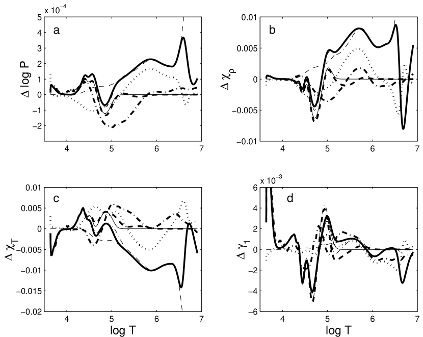
Figure 12: Relative difference between thermodynamic quantities for the H-He mixture in a test with setting the occupation probability of the ground states $w_{1s}=1$ (see text for a description). Differences are in the sense (X - X${}_{\rm MHD_{\rm GS}}$) / X${}_{\rm MHD_{\rm GS}}$. Thick Dashed Line: MHD; Thick Dashed-dotted Line: OPAL; Dotted Line: CEFF; Thin Dashed-dotted Line: MHD_W1; Thin Dashed Line: MHD_GS,W1; Thin Solid Line: MHD_He:GS; Thick Solid Line: MHD_He:GS,W1.

For this test we have used a pure hydrogen-helium mixture. For consistency with the work by ND98, we have taken their run of temperature and density, which corresponds roughly to the solar convection zone (here we refer to these conditions as “solar track”, to distinguish it from the more precise concept of a solar model used in other figures). Our results are shown in Fig. 12. Besides the previously defined labels OPAL, CEFF, and MHD, here the label MHD_GS for the standard MHD internal partition function of hydrogen and helium truncated to the ground state term (see also ND98). MHD_W1 and MHD_GS,W1 are the same as MHD and MHD_GS, respectively, except that in them the occupation probabilities of all the ground states are set to be $1$. The label MHD_He:GS refers to a truncation to the ground state term of the helium internal partition function only. Similarly, MHD_He:GS,W1 refers to ground-states occupation probabilities in MHD_He:GS that are set to $1$. We again stress that the absence of the possibility to model pressure ionization makes the MHD_GS,W1 model quite unphysical. Indeed, it is found to deviate significantly from all other models at sufficiently high densities, where pressure ionization matter.

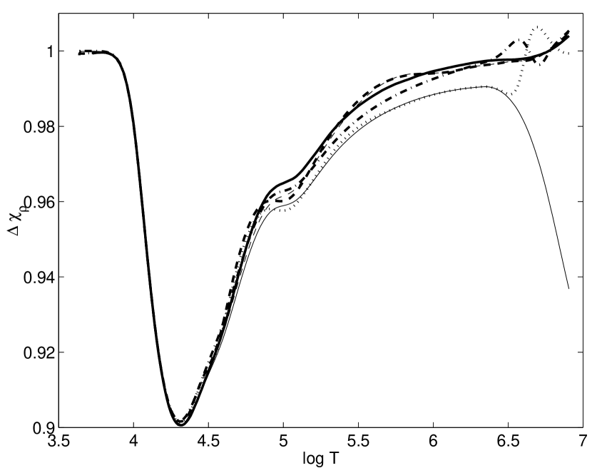
Figure 13: Absolute value of $\chi_{\rho}$ for the H-He mixture in a test with setting the occupation probability of the ground states $w_{1s}=1$ (see text for a description). Thick Dashed Line: MHD; Thick Solid Line: OPAL; Dashed-dotted Line: CEFF; Dotted Line: MHD_W1; Thin Solid Line: MHD_GS,W1; Thin Dashed Line: MHD_GS.

In Fig. 13, we see that the ND98-wiggle between $\log T=4.5$ and $5.5$ shows up more distinctly when the occupation probability of the ground state is set to $1$. This clearly confirms the conclusion by ND98 that the wiggle must be a pure excited-states effect. An occupation probability of the ground states different from $1$ actually happens to reduce the wiggle. From Fig. 12 (a-c) we can see that MHD_He:GS model is very close to MHD model, and MHD_He:GS,W1 is very close to MHD_W1. The presence of helium does not change very much, which is another confirmation of the conclusion by ND98 that the wiggle is an excited-states effect of pure hydrogen.

Furthermore, it can be seen from Fig. 12 (a-c) that the effect of the ground-state occupation probability shows up at temperatures $\log T>4.5$, and it is most significant for $5<\log T<6.6$. Although none of our results appears to fit the OPAL equation of state closely (not surprising with our academic exercise), nonetheless it follows that setting ground-state occupation probabilities to $1$ does bring the results somewhat closer to OPAL. It could well be that in the MHD occupation probability formalism with $w_{is}$ of Hummer and Mihalas (1988) [see Eq.(2)], the ground states might be too strongly perturbed.

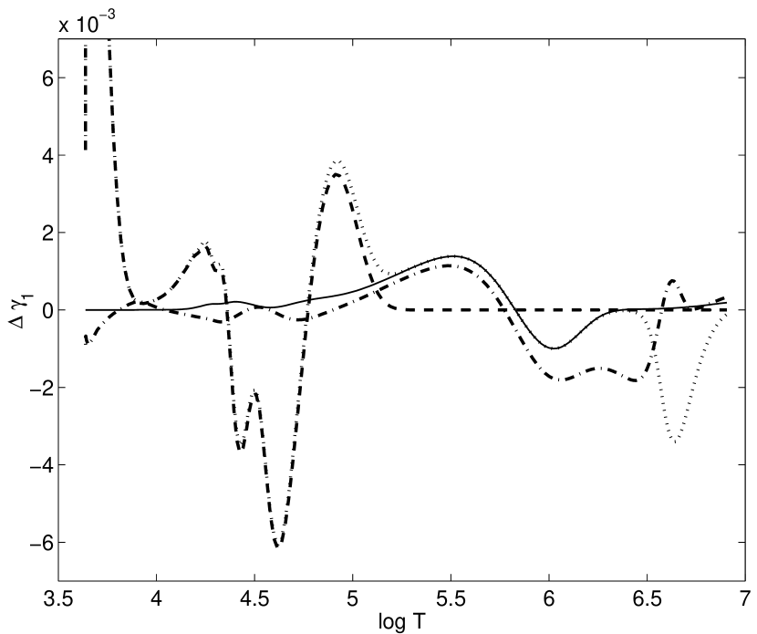
Figure 14: Relative difference between thermodynamic quantities for the pure hydrogen plasma in a test with setting the occupation probability of the ground states $w_{1s}=1$ (see text for a description). Differences are in the sense (X - X${}_{\rm MHD_{\rm GS}}$) / X${}_{\rm MHD_{\rm GS}}$. Dashed Line: MHD; Dashed-dotted Line: CEFF; Dotted Line: MHD_W1; Solid Line: MHD_GS,W1.

Another interesting feature is shown in Fig. 12 (d) in the temperature range $\log T=5.2$ to $\log T=6.0$. By comparison with Fig. 10, we see that the difference in $\gamma_{1}$ between MHD and MHD_GS,W1 suspiciously mimics the difference between MHD and OPAL in that region. Now, this is precisely the region where helioseismic inversions [see, e.g. Basu, Däppen and Nayfonov (1999)] have given evidence that the MHD equation of state is not as good as OPAL. In both cases, the intersection of both MHD versions with OPAL happens at about the same temperature ($\log T\approx 5.8$), and their slopes are about the same. This is an indication that, even if the extreme case of $w_{1s}=1$ in the ground states can not be an overall improvement of the MHD the equation of state, the specific ground-state occupation numbers $w_{is}$ of Hummer and Mihalas (1988) [see Eq.(2)] should be improved, most likely so that they will be closer to $1$. Fig. 14 also tells us that it is the choice of occupation probability of the ground states of hydrogen that is responsible for the difference between MHD and OPAL from $\log T=5.5$ to $\log T=6.0$. This result shows another direction in which the MHD equation of state can be improved, namely by inclusion of a more realistic pressure-ionization mechanism, likely based on a hard sphere model [see, for instance, Saumon and Chabrier (1992)]. Such a procedure could then assure physical consistency even if $w_{1s}=1$.

Special attention is also in order for the cases MHD_GS,W1 and MHD_He:GS,W1, in the temperature range of $5.2<\log T<5.6$, shown in Fig. 12 (d). Both these cases are close to OPAL. First, one can realize that it is the contribution of the excited states of helium that causes the behavior of the $\Delta\gamma_{1}$ line at the low-temperature end. Then, in this figure the wiggly feature from $4.0<\log T<5.2$ is once again the contribution of the excited states of hydrogen. If we assume that OPAL is the better equation of state around the temperature of $\log T\approx 5.8$ then the occupation probability expression used by Hummer and Mihalas (1988) might indeed have altered the partition function of the ground states too strongly.

4.2 Effect of the $\tau$ correction

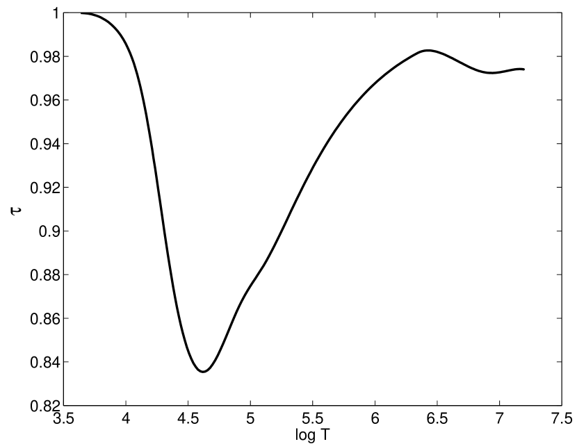
Figure 15: The $\tau$ correction in the solar convection zone.

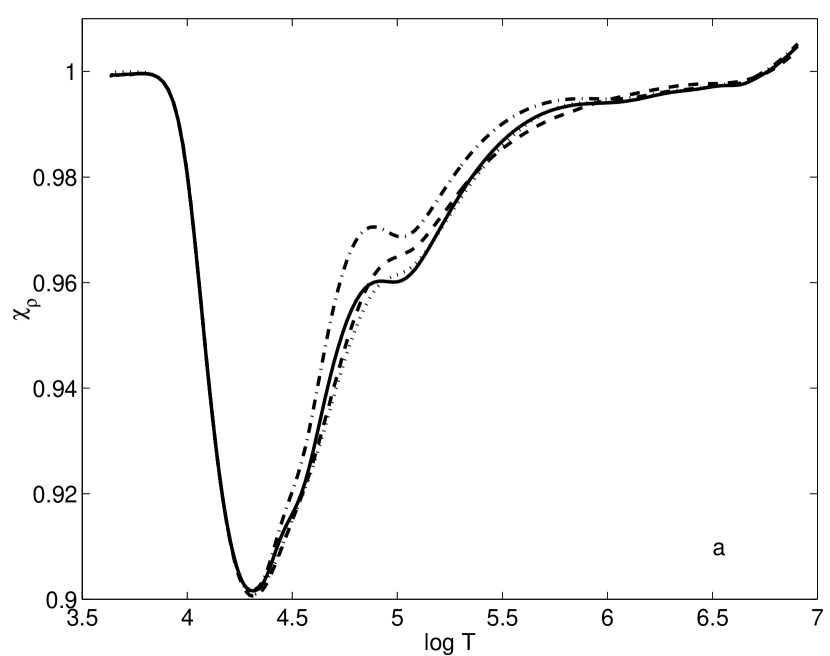
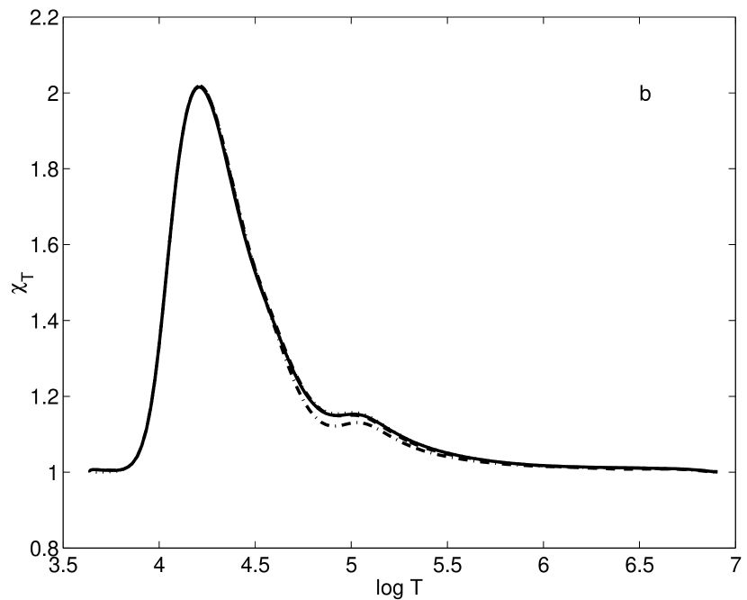
Figure 16: Values of $\chi_{\rho}$ and $\chi_{T}$ for the H-He mixture with and without $\tau$ correction inside the sun. Solid Line: MHD; Dotted Line: MHD_GS; Dashed Line: OPAL; Dashed-dotted Line: MHD with $\tau$ correction.

Another numerical experiment was dedicated to the validity of the $\tau$ correction to the Debye-Hückel term, such as employed in the MHD equation of state, but also in CEFF. As mentioned in section 1, the $\tau$ correction is conventionally added (Graboske, Harwood and Rogers, 1969) to remedy the effects of the divergence of the Debye potential at $r=0$. The net effect of the $\tau$ correction is to prevent the negative Debye-Hückel pressure correction from exceeding the ideal-gas pressure which would, at very high densities, cause a negative total pressure. In Fig. 15, we have plotted the value of $\tau$ for our solar model. Because the Debye-Hückel correction reaches its maximum in the middle of the solar convection zone, $\tau$ is there also bigger than elsewhere. In parallel, in that region $\chi_{\rho}$ is enhanced and $\chi_{T}$ reduced with respect to the other equations of state that have no $\tau$ correction (Fig. 16).

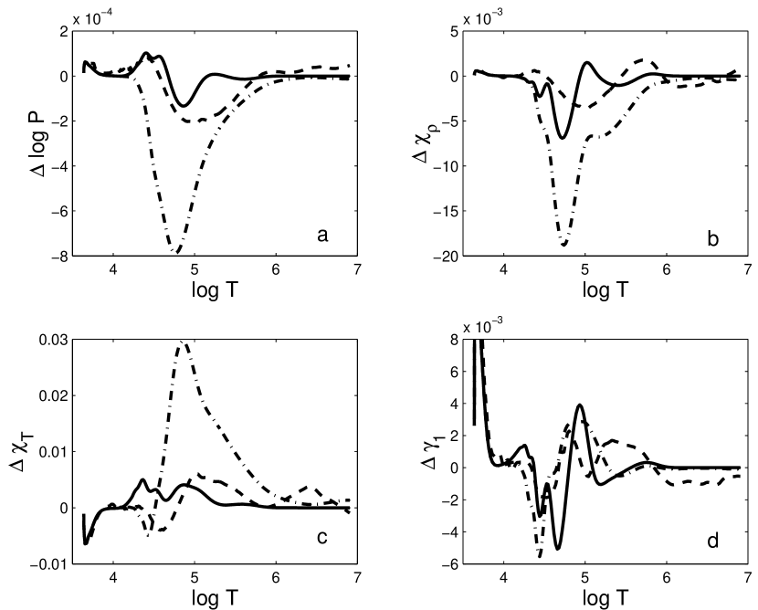
Figure 17: Relative difference of thermodynamic quantities for the H-He mixture with and without $\tau$ correction inside the sun. Differences are in the sense (X - X${}_{\rm MHD_{\rm GS}}$) / X${}_{\rm MHD_{\rm GS}}$. Solid Line: MHD; Dashed Line: OPAL; Dashed-dotted Line: MHD with $\tau$ correction.

A comparison of Fig. 17 (a-c) with Fig. 15 makes one realize that the $\tau$ contribution shows up clearly in pressure, $\chi_{\rho}$ and $\chi_{T}$, revealing how these thermodynamic quantities differ from those of equations of state without a $\tau$ correction. The $\tau$ correction leads to a significant change of the thermodynamic quantities in the solar convection zone. If one assumes that OPAL (which does not contain a $\tau$ correction) is in all respects quite close to the true equation of state in this temperature range, one can conclude that a $\tau$ correction would lead to inconsistent quantities $\chi_{\rho}$ and $\chi_{T}$ . However, in $\gamma_{1}$ [Fig. 17 (d)], the behavior of the $\tau$ correction is more complicated and concealed. That is certainly one of the reason why helioseismic studies so far have not had problems with the $\tau$ correction. For instance, very successful solar models have been constructed with CEFF and MHD. As a word of caution we mention, however, that the recipe of improving the MHD equation of state by simply removing its $\tau$ correction would not work in all stellar applications. For the sun it does work, because nowhere inside does the Debye-Hückel term come even close to cause negative pressure. In contrast, an application of the MHD equation of state to the physical conditions of low-mass stars would be confronted with this pathology, and adding the $\tau$ correction is a must, already for formal reasons, independent of physical merit. Incidentally, the MHD equation of state with a $\tau$ correction has turned out to be a useful working tool for low-mass stars (Charbonnel et al., 1999), but this might have been due to fortuitous circumstances. For a more realistic physical description, high-order contributions in the Coulomb interaction beyond the Debye-Hückel theory will be needed.

5 Conclusions

The first part of the paper has been dedicated to the influence of heavy elements in thermodynamic quantities. To isolate the contribution of a selected heavy elements separately, we have compared the results from a H-He-C mixture with those of a H-He mixture. It has emerged that for temperatures between $4.5<\log T<5.5$ (region “A” in Fig. 6 and Fig. 7), the thermodynamic quantities are very sensitive to the detailed physical treatment of heavy elements, in particular regarding the excited states of all atoms and ions of the heavy elements. These findings carry an important diagnostic potential to use the sun as a laboratory to constrain physical theories of atoms and ions immersed in hot dense plasmas.

However, we have also found that not all physical effects of heavy-elements can be detected with helioseismic studies. The reason is that in a realistic mixture with many heavy elements, at certain places in the solar convection zone, the profile of the relevant adiabatic gradient is significantly smoother than for less realistic artificial mixtures which contain a smaller number of heavy elements. As a consequence, in some locations, the adiabatic gradient can become quite independent of details of the physical treatment of the species. Such a property is welcome news for solar modelers, because it reduces the uncertainty due to the equation of state. A prime beneficiary of this enhanced precision will be the helioseismic helium and heavy-element abundance determination. To this purpose, we have identified in the adiabatic gradient a useful device in the form of a prominent, largely model-independent feature of heavy elements. This feature is found at temperatures around $5.5<\log T<6.5$ (region “B” in Fig. 6 and Fig. 7), corresponding roughly to the base of solar convection zone, where each heavy element exhibits its own ionization profile. We verified that these profiles are indeed quite independent of the details in the physics. They can serve as tracers for heavy elements, and they harbor the potential for a helioseismic determination of the relative abundance of heavy elements in the solar convection zone.

The second part of the paper deals with related issues. It is no surprise that the major contribution of the heavy elements to pressure is given by the total number particles involved. These are nuclei and the electrons released by ionization, which is mainly determined by temperature and the relevant ionization energies. Somewhat less expected is the result that with a larger number of heavy elements, the profile of thermodynamic quantities becomes smoother than in the case of a low number (one or two) representative heavy elements. In a quantitative study, we found that 6-element mixtures, which are still widely used in solar modeling, may contain errors in $\gamma_{1}$ of up to $3\times 10^{-4}$ due to the insufficient number of heavy elements. Such a discrepancy does matter in present helioseismic studies (section 3.4). We conclude that in order to avoid this error, the element mixture must contain at least 10 of the most abundant elements.

In a third part, rather as a by-product of the present study, we discovered one important reason why in helioseismic studies, the MHD equation of state does not produce as good results as the OPAL equation of state. We developed an unphysical diagnostic formalism, where the occupation probability of the ground states of all species was left untouched at $1$. With this simple tool, we have on the one hand confirmed the conjectures of ND98 about the importance of the ground-state contribution compared to that of the excited states. On the other hand, we have also shown that the difference between the MHD and OPAL equations of state around $\log T\approx 5.8$ appears to be due to MHD’s specific choice of the occupation probability of the ground state of hydrogen. We have realized that the ground-state contribution clearly moves away the MHD model both from helioseismologically determined values and OPAL. This result suggests that the specific occupation probability adopted by Hummer and Mihalas (1988) might perturb the ground states (and perhaps also the low-lying excited states) too strongly.

In a final part, and as an another by-product, we have obtained quantitative results about the effect of the $\tau$ correction term, which is sometimes added to Debye-Hückel theory. We confirm earlier conjectures (Baturin et al., 1995) that the $\tau$ correction causes a significant spurious effect in the solar equation of state and is therefore inadmissible. The $\tau$ correction should therefore be taken out of the MHD equation of state (and CEFF for that matter). Such a remedy will be acceptable for solar applications, because of the overall smallness of the Debye-Hückel correction in the sun. However, some form of a $\tau$ correction is still be required for low-mass stellar modeling with the MHD and CEFF equations of state, because it has to prevent the total pressure from becoming negative at high densities and relatively low temperatures. We note in passing that the OPAL equation of state does not need a $\tau$ correction because it contains genuine higher-order Coulomb correction terms. The major discrepancy between MHD and OPAL – other than the aforementioned ground-state effect – is not an absence of higher-order Coulomb terms in MHD, but the presence of incorrect ones in the form of the $\tau$ correction. The MHD equation of state should be upgraded to include higher-order Coulomb contributions.

Table 1: Chemical composition of the heavy elements in the 6-element mixture

Element	Relative Mass Fraction	Relative Number Fraction
Carbon	0.1906614	0.2471362
Nitrogen	0.0558489	0.0620778
Oxygen	0.5429784	0.5283680
Neon	0.2105114	0.1624178

Table 2: Properties of the solar models used in Fig. 10 (see text).

Model	Equation	Radius	Convective	$Y_{\rm s}$	$r_{\rm cz}/R_{\odot}$
	of State	Mm	Flux
M1	MHD	695.78	CM	0.2472	0.7145
M2	MHD	695.99	CM	0.2472	0.7146
M3	MHD	695.51	CM	0.2472	0.7145
M4	MHD	695.78	MLT	0.2472	0.7146
M5	OPAL	695.78	CM	0.2465	0.7134
M6	OPAL	695.99	CM	0.2465	0.7135
M7	OPAL	695.51	CM	0.2466	0.7133
M8	OPAL	695.78	MLT	0.2465	0.7135

Figure 10: Intrinsic difference between $\gamma_{1}$ obtained from an inversion of helioseismological data (Basu, Däppen and Nayfonov, 1999), and $\gamma_{1}$ of the solar models M1–M8 listed in Table 2, in the sense “sun – model”. The intrinsic difference is due to the change in the equation of state alone (see text). Filled points label results from MHD models, empty ones OPAL. Lines have been drawn through results of models M1 and M5 to guide the eye. For the sake of clarity, error bars have been drawn only on two sets of results.

References

- Antia and Chitre (1998) Antia, H. M. and Chitre, S. M. 1998, A&A, 339, 239 – 251.
- Bahcall and Pinsonneault (1992) Bahcall, J. N. and Pinsonneault, M. H. 1992, Reviews of Modern Physics, 64, 885
- Basu and Christensen-Dalsgaard (1997) Basu, S. and Christensen-Dalsgaard, J. 1997, A&A, 322, L5 – L8.
- Basu, Däppen and Nayfonov (1999) Basu, S., Däppen, W. and Nayfonov, A. 1999, ApJ, 518, 985
- Baturin et al. (2000) Baturin, V. A., Däppen, W., Gough, D. O. and Vorotsov, S. V. 2000, M.N.R.A.S., 316, 71
- Baturin et al. (1995) Baturin, V. A., Däppen, W., Wang, X. and Yang, F. 1995, Stellar Evolution: What Should be Done, 32nd Liége International Astrophysical Collo., ed. A. Noels, D. Fraipont-Caro, M. Gabriel, N. Grevesse and P. Demarque, (Université de Liége: Liége, Belgium), 33
- Brun, Turck-Chièze and Zahn (1999) Brun, A. S., Turck-Chièze, S. and Zahn, J. P. 1999, ApJ, 525, 1032
- Charbonnel et al. (1999) Charbonnel, C., Däppen, W., Bernasconi, P., Maeder, A., Meynet, G., Schaerer, D. and Mowlavi, N. 1999, A&AS, 135, 405
- Canuto and Mazitelli (1991) Canuto, V. M., and Mazzitelli, I. 1991, ApJ, 370, 295
- Christensen-Dalsgaard and Däppen (1992) Christensen-Dalsgaard, C. and Däppen, W. 1992, A&A Rev., 4, 267
- Christensen-Dalsgaard, Däppen and Lebreton (1988) Christensen-Dalsgaard, C., Däppen, W. and Lebreton, L. 1988, Nature, 336, 634
- Christensen-Dalsgaard et al. (1996) Christensen-Dalsgaard, J., Däppen, W., and the GONG Team 1996, Science, 272, 1286
- Cox, Guzik and Kidman (1989) Cox, A. N., Guzik, J. A. and Kidman, R. B., 1989, ApJ, 342, 1187
- Däppen (1996) Däppen, W. 1996, Bull. Astr. Soc. India, 24, 151
- Däppen et al. (1993) Däppen, W., Gough, D. O., Kosovichev, A. G. and Rhodes, E. J. Jr. 1993, Inside the Stars, ed. W. W. Weiss and A. Baglin, Proc. IAU Colloq. 137, (ASP: San Fransisco), 304
- Däppen, Mihalas and Hummer (1988) Däppen, W., Mihalas, D., and Hummer, D. G. 1988, ApJ, 332, 261
- Debye and Hückel (1923) Debye, P. and Hückel, E. 1923, Physic. Z., 24, 185
- Eggleton, Faulkner and Flannery (1973) Eggleton, P. P., Faulkner, J. and Flannery, B. P. 1973, A&A, 23, 325
- Elliot and Kosovichev (1998) Elliot J. R. and Kosovichev A. G. 1998, ApJ, 500, L199
- Gong and Däppen (2000) Gong, Z. G. and Däppen, W. 2000, The Impact of Large-scale Surveys on Pulsating Star Research, ed. L. Szabados and D. Kurtz, Proc. IAU Colloq. 176, (ASP: San Francisco), 388
- Gong, Däppen and Zejda (2001) Gong, Z. G., Däppen, W. and Zejda, L. 2001, ApJ, 546, 1178
- Gough (1984) Gough, D. O. 1984, Mem. Soc. Astron. Ital., 55, 13
- Graboske, Harwood and Rogers (1969) Graboske, H. C. Jr., Harwood, D. J. and Rogers, F. J. 1969, Phys. Rev., 186, 210
- Grevesse and Noels (1993) Grevesse, N. and Noels, A. 1993, in Origin and evolution of the Elements, eds N. Prantzos, E. Vangioni-Flam and M. Cassé (Cambridge: Cambridge Univ. Press), 15 – 25.
- Grevesse and Sauval (1998) Grevesse, N. and Sauval, A. J. 1998, Space Science Reviews, 85, 161
- Guzik and Swenson (1997) Guzik, J. A. and Swenson, F. J. 1997, ApJ, 491, 967
- Hummer and Mihalas (1988) Hummer, D. G., and Mihalas, D. 1988, ApJ, 331, 794
- Iglesias and Rogers (1996) Iglesias, C. A. and Rogers, F. J. 1996, ApJ, 464, 943 – 953.
- Irwin et al. (2001) Irwin, A., Swenson, F. J., VanderBerg, D. and Rogers, F. J., 2001, in preparation
- Kippenhahn and Weigert (1990) Kippenhahn, R. and Weigert, A. 1990, Stellar Structure and Evolution, Springer-Verlag: Berlin
- Kurucz (1991) Kurucz, R. L. 1991, in Stellar atmospheres: beyond classical models, eds. Crivellari, L., Hubeny, I. and Hummer, D. G., (NATO ASI Series, Kluwer, Dordrecht), 441 - 448
- Lebreton and Däppen (1988) Lebreton, Y. and Däppen, W. 1988, Seismology of the Sun and Sun-like Stars, ed. V. Domingo and E. J. Rolfe, ESA SP-286, (ESA Publications Division: Noordwijk, the Netherlands), 661
- Michaud and Vauclair (1991) Michaud, G. and Vauclair, S. 1991, Solar Interior and Atmosphere, ed. A. N. Cox, W. C. Livingston and M. S. Matthews, (Tuscon: University of Arizona Press), 304
- Mihalas, Däppen and Hummer (1988) Mihalas, D., Däppen, W., and Hummer, D. G. 1988, ApJ, 331, 815
- Mihalas et al. (1990) Mihalas, D., Hummer, D. G., Mihalas, B. W. and Däppen, W. 1990, ApJ, 350, 300
- Nayfonov and Däppen (1998) Nayfonov, A. and Däppen, W. 1998, ApJ, 499, 489
- Nayfonov et al. (1999) Nayfonov, A., Däppen, W., Mihalas, D., and Hummer, D. G. 1999, ApJ, 526, 451
- Proffitt (1994) Proffitt, C. R. 1994, ApJ, 425, 849
- Richard et al. (1996) Richard, O., Vauclair, S., Charbonnel, C. and Dziembowski, W. A. 1996, A&A, 312, 1000
- Rogers (1986) Rogers, F. J. 1986, ApJ, 310, 723
- Rogers, Swenson and Iglesias (1996) Rogers, F. J., Swenson, F. J., and Iglesias, C. A. 1996, ApJ, 456, 902
- Saumon and Chabrier (1992) Saumon, D. and Chabrier, G. 1992, Phys. Rev. A, 46, 2084
- Shibahashi, Noels and Gabriel (1983) Shibahashi, H., Noels, A. and Gabriel, M. 1983, A&A, 123, 283
- Thoul, Bahcall and Loeb (1994) Thoul, A. A., Bahcall, J. N. and Loeb, A. 1994, ApJ, 421, 828
- Ulrich (1982) Ulrich, R. K. 1982, ApJ, 258, 404
- Vorontsov et al. (1994) Vorontsov, S. V., Baturin, V. A., Gough, D. O. and Däppen, W. The Equation of State in Astrophysics, ed. G. Chabrier and E. Schatzmann, Proc. IAU Colloq. 147, (Cambridge: Cambridge University Press), 545