THE ROLE OF ACTIVE REGIONS IN THE GENERATION OF TORSIONAL OSCILLATIONS

Abstract

We present a model for torsional oscillations where the inhibiting effect of active region magnetic fields on turbulence locally reduces turbulent viscous torques, leading to a cycle- and latitude-dependent modulation of the differential rotation. The observed depth dependence of torsional oscillations as well as their phase relationship with the sunspot butterfly diagram are reproduced quite naturally in this model. The resulting oscillation amplitudes are significantly smaller than observed, though they depend rather sensitively on model details. Meridional circulation is found to have only a weak effect on the oscillation pattern.

1 Introduction

Solar torsional oscillations, discovered by Howard and LaBonte (1980), consist of alternating latitudinal bands of faster and slower than average rotation in the solar photosphere, distributed symmetrically to the equator, and migrating during the solar cycle. Early investigations (LaBonte and Howard, 1981; Snodgrass and Howard, 1985) revealed a characteristic phase relationship between these torsional waves, of wavenumber $\sim 2/$hemisphere, and the sunspot butterfly diagram: sunspot activity varies approximately in phase with the latitudinal shear $\partial\omega/\partial\theta$. The characteristic amplitude of the oscillations is order of $0.1\,\%$, or a few nHz.

Since the first seismic detection of torsional waves from $f$-mode splittings by Kosovichev and Schou (1997), helioseismic observations have brought great advance in the study of these oscillations (Schou et al., 1998; Howe et al., 2000). With these methods the depth dependence of these motions could also be studied. It was found that the motions extend to about the upper third of the solar convective zone, while coherent torsional oscillations seem to disappear below a depth of about 70 Mm (Antia and Basu, 2000; Howe et al., 2001). These studies also shed light on the long disputed high latitude behaviour of the oscillations, demonstrating the existence of a poleward propagating branch at high latitudes (Howe et al., 2001). This parallels the existence of a similar branch in the sunspot/facula butterfly diagram, and it explains earlier propositions of the coexistence of a $\sim 1/$hemisphere modulation with the torsional waves.

Most theoretical attempts to interpret the torsional oscillations attribute them to some feedback effect of the magnetic fields on the differential rotation. (See, however, Tikhomolov, 2001 for a dissenting view.) Kitchatinov et al. (1999) plausibly classify the models as “macrofeedback” and “microfeedback” scenarios, depending on whether the feedback is due to the Lorentz force associated with the large-scale magnetic field or to the inhibiting effect of magnetic fields on the (turbulent) angular momentum transport mechanisms responsible for differential rotation. The first macrofeedback models were proposed by Schüssler (1981) and Yoshimura (1981), while the latest, most extensive and detailed such models were developed by Covas et al. (2000, 2001). Microfeedback models have been elaborated by the Potsdam–Irkutsk group (e.g. Küker, Rüdiger, and Pipin, 1996; Kitchatinov et al., 1999).

All the models of torsional oscillations proposed to date are based on a complete mean-field dynamo. At first sight this may seem natural: however, it is not necessarily a desirable feature of such a model, for two reasons. Firstly, there is still wide disagreement concerning just how the solar dynamo operates (cf. review by Petrovay, 2000). Thus, the use of a particular dynamo model introduces a high degree of arbitrariness into the study of torsional oscillations. Second, the recently discovered shallowness of the torsional oscillation phenomenon suggests that near-surface magnetic fields play a dominant role in their generation. These fields are directly observable in the photosphere, which not only makes it possible to dispense with the use of a dynamo model to calculate them, but in fact it demonstrates that a purely mean-field calculation may perhaps never grasp the most important factors modulating the angular momentum distribution near the surface. Indeed, from observations it is well known that the overwhelming majority of the cycle-dependent part of photospheric magnetic flux density $\overline{|\mbox{\bf B}|}$ is in the form of active regions (Harvey, 1993, 1994). The dynamics of the thick active region flux tubes is governed by volume forces such as buoyancy and the curvature force; it is therefore largely independent of the external turbulence, and it cannot be described by one-fluid models like mean field theory, in contrast to the “passive” fields consisting of thin fibrils (cf. Petrovay, 1994).

The aim of this paper is to investigate whether active regions (ARs) can play a role in the modulation of angular momentum distribution in the shallow layers of the convective zone. An obvious argument against such a role is that the volume filling factor of the magnetic flux tubes forming ARs is small throughout the convective zone. This is indeed the case if one regards the volume actually magnetized; however, the presence of a sufficiently dense network of individual flux tubes (e.g. a “magnetic tree” below a large active region or an ensemble of ephemeral active regions) may significantly affect the flow throughout that network, so that the influence of ARs may extend to a much larger fluid volume. This implies that the rotational modulation induced by ARs, if any, should not work by the direct action of Lorentz forces on the large-scale flow but by the spatially more extended influence on turbulent angular momentum transport. In other words, AR-induced rotational modulation will be a microfeedback effect.

In a simplified description, this feedback will essentially consist in a suppression of turbulent viscosity. (Another possible mechanism by which ARs may modify the differential rotation may be their influence on the large scale flow.) Indeed, there is now a rather wide consensus that the solar differential rotation is mainly generated by the $\Lambda$-effect in the deep layers of the convective zone (possibly aided by the return flow of meridional circulation; Rekowski and Rüdiger, 1998; Gilman, 2000). The pole-to-equator transport of angular momentum in the deep layers is compensated by a transport of the opposite sense in the upper half of the convective zone, mainly due to turbulent viscosity (and possibly to meridional circulation). It is this latter transport that the active regions field may interfere with, so that in a simplified approach their influence may be represented by a reduction of the turbulent viscosity. This reduction is not expected to extend very deep into the convective zone as the “branches” of the magnetic trees underlying active regions are thought to separate at a depth of about 50 Mm only.

The structure of our paper is the following. In Section 2 we describe our model and discuss the problem of the quantitative formulation of the AR-induced reduction of viscosity. In Section 3 we present the resulting torsional oscillation profiles as functions of latitude, radius and time, for various assumptions on the reduction of diffusivity, with and without meridional circulation. Finally, Section 4 concludes the paper.

2 The Model

2.1 Geometry

Our computational volume is a spherical half-shell below the solar surface. Axial and equatorial symmetry is assumed. The bottom of the shell is placed to a depth of $z_{0}=160\,$Mm. It is assumed that the $\Lambda$-effect operates below our shell only, its effect being described by a prescribed differential rotation profile at the lower boundary. The bottom depth of 160 Mm may seem too deep for this assumption to be valid; however, in order to convincingly show that the torsional waves appearing in our model are confined to depths less than 70 Mm, the lower boundary had to be placed sufficiently deep below that level.

2.2 Equations

In order to describe differential rotation in the solar interior, it is useful to write the equations in a frame rotating with a fixed angular velocity $\Omega_{0}$. The equation of motion reads

$$\partial_{t}\mathbf{v}+\left(\mathbf{v}\cdot\nabla\right)\mathbf{v}+2\vec{\Omega}_{0}\times\mathbf{v}=-\nabla V-\frac{1}{\rho}\nabla p+\frac{1}{\rho}\nabla\cdot\mathbf{\tau},$$ (1)

where $\rho$ and $p$ are density and pressure, respectively, v is the fluid velocity, $V$ is the gravitational potential, and $\tau$ is the viscous stress tensor. This equation is supplemented by the constraint of mass conservation (anelastic approximation):

$$\nabla\cdot(\rho\mathbf{v})=0.$$ (2)

As a result of the anelastic approximation, the circulation in the spherical shell may be represented by a stream function $\Psi$ so that the velocity field can be written as

$$v_{r} = \frac{1}{\rho r^{2}\sin\theta}\partial_{\theta}\Psi$$ (3)

$$v_{\theta} = -\frac{1}{\rho r\sin\theta}\partial_{r}\Psi$$ (4)

$$v_{\phi} = r\sin\theta\,\omega,$$ (5)

where $v_{r}$, $v_{\theta}$ and $v_{\phi}$ are, respectively, the radial, meridional and azimuthal components of the velocity, and $\omega$ is the angular velocity in our rotating frame. In order to present more transparent equations we write the stream function in the following form:

$$\Psi=\psi(r)\sin^{2}\theta\cos\theta$$ (6)

$$\psi(r)=-0.01\,R_{\odot}^{2}\exp\left[-500\left(\frac{r-r_{m}}{R_{\odot}}\right)^{2}\right],$$ (7)

where $r_{m}=r_{str}+(R_{\odot}-r_{str})/2$ and $r_{str}=520\,$Mm. The parameters and form of this formula were designed to mimick the observed properties of meridional circulation, with a peak amplitude of $\sim 20\,$m/s at the surface (Komm, Howard, and Harvey, 1993; Latushko, 1994).

Figure 1: Streamlines of the meridional circulation prescribed in eq. (6) (clockwise circulation). The dotted line is the bottom of our computational domain.

The components of the viscous stress tensor appearing in the azimuthal component of the Navier-Stokes equation read

$$\tau_{\theta\phi} = \tau_{\phi\theta}=\rho\nu\frac{\sin\theta}{r}\,\partial_{\theta}\left(\frac{v_{\phi}}{\sin\theta}\right),$$ (8)

$$\tau_{\phi r} = \tau_{r\phi}=\rho\nu r\,\partial_{r}\left(\frac{v_{\phi}}{r}\right),$$ (9)

where $\nu$ is the viscosity. Thus, the azimuthal component of the equation of motion, including the effects of diffusion, Coriolis force and meridional circulation, becomes

$$\partial_{t}\omega = \left(\partial_{r}\nu+4\frac{\nu}{r}+\frac{\nu}{\rho}\partial_{r}\rho\right)\partial_{r}\omega+\nu\partial^{2}_{r}\omega+\frac{3\nu\cos\theta}{r^{2}\sin\theta}\partial_{\theta}\omega$$

$$+ \frac{\nu}{r^{2}}\partial^{2}_{\theta}\omega+M+C$$

$$M = \frac{\psi\omega}{r^{3}\rho}\left(2\sin^{2}\theta-4\cos^{2}\theta\right)+\frac{\psi\partial_{r}\omega}{r^{2}\rho}\left(\sin^{2}\theta-2\cos^{2}\theta\right)$$

$$+ \frac{\partial_{r}\psi}{r^{2}\rho}\left(\partial_{\theta}\omega\cos\theta\sin\theta+2\omega\cos^{2}\theta\right)$$

$$C = \frac{2\Omega_{0}\psi}{r^{3}\rho}\left(\sin^{2}\theta-2\cos^{2}\theta\right)+\frac{2\Omega_{0}\cos^{2}\theta\partial_{r}\psi}{r^{2}\rho},$$ (12)

where $M$ denotes the terms associated with the advection by meridional circulation and $C$ denotes the terms associated with the Coriolis force.

2.3 Boundary and initial conditions

For the integration of equation (2.2) boundary conditions on $\omega$ are needed. At the pole and the equator symmetry is required:

$$\partial_{\theta}\omega=0\qquad\mbox{at }\theta=0^{\circ}\mbox{ and }\theta=90^{\circ}$$ (13)

At the lower boundary of our computational volume, $r_{\mbox{\scriptsize{in}}}=R_{\odot}-z_{0}=540\,$Mm, we suppose that the rotation rate can be described with the same expression as on the surface. In accordance with the observations of Schou et al. (1998), the following expression is used for $\Omega_{\mbox{\scriptsize{surf}}}$:

$$\frac{\Omega_{\mbox{\scriptsize{surf}}}}{2\pi}=455.4-52.4\cos^{2}\theta-81.1\cos^{4}\theta\hskip 5.69046pt\mbox{nHz}.$$ (14)

This is used to give the inner boundary condition on $\omega$,

$$\Omega_{0}+\omega=\Omega_{\mbox{\scriptsize{surf}}}$$ (15)

$\Omega_{0}$ is (arbitrarily) chosen as the rotation rate in the radiative interior below the tachocline. On the basis of helioseismic measurements, this value is equal to the rotation rate of the convection zone at a latitude of about $30^{\circ}$, corresponding to $\Omega_{0}/2\pi=437$ nHz.

Finally, the upper boundary condition on $\omega$, at $r_{\mbox{\scriptsize{surf}}}=R_{\odot}$ follows from the requirement that the tangential viscous stress $\tau_{\phi r}$ must vanish at the surface:

$$\partial_{r}\omega=0\hskip 14.22636pt\mbox{at}\hskip 2.84544ptr=r_{\mbox{\scriptsize{surf}}}.$$ (16)

The initial conditions chosen for all calculations are

$$\omega(r,\theta,t=0)= \Omega_{\mbox{\scriptsize{surf}}}-\Omega_{0}\qquad \mbox{at }r=r_{\mbox{\scriptsize{in}}}$$

$$\omega(r,\theta,t=0)= 0\hskip 51.21504pt \mbox{at }r>r_{\mbox{\scriptsize{in}}}$$ (17)

2.4 Viscosity suppression

Active regions are thought to originate from the emergence of strong magnetic flux loops, driven by the buoyant instability of toroidal flux tubes. This emergence process is quite well investigated (see e.g. Moreno-Insertis, 1994), and a comparison of theoretical calculations with observations has allowed to draw the conclusion that large AR originate from the rise of toroidal flux tubes with field strengths of $\sim 10^{5}\,$G and magnetic flux $\sim 10^{22}\,$Mx, lying at the bottom of the convective zone. Observational and theoretical evidence alike suggest that a few tens of megameters below the surface, the rising loop is fragmented into a tree-like structure, leading to the observed size spectrum of magnetic concentrations in AR from large spots through pores and knots down to facular points. The probable cause of the fragmentation is that the field strength in the top of the loop is reduced below the local equipartition field strength, allowing external turbulence to penetrate the tube and fragment it by the mechanism of flux expulsion.

The origin of ephemeral active regions (EAR) is less clear, although this is an important issue for our present purposes, as EAR contribute to the observed photospheric magnetic flux density by an amount comparable to large AR. Their properties suggest that EAR may be the result of the buoyant instability of thinner and weaker toroidal flux tubes, situated at shallower depths in the convective zone. One possibility is that this shallower and more fragmented toroidal field, in turn, results from the “explosion” of large emerging flux loops with lower initial field strengths and fluxes than those causing large AR (Moreno-Insertis, Caligari, and Schüssler, 1995). While this is not the only possibility, tentatively accepting it simplifies our present problem, as in this case the subsurface structure corresponding to EAR collectively can also be thought of as a collection of magnetic trees, just perhaps with somewhat deeper and more extended “crowns” than in the case of large AR.

Figure 2: Radial profiles of the viscosity using the values $N_{AR}=3$, $\theta=60^{\circ}$ in equation (18). Solid: $D_{0}=z_{0}=80\,$Mm. Dashed: $D_{0}=z_{0}=50\,$Mm

The above considerations suggest that a simplified description of the subsurface magnetic structures that give the bulk of the flux density in the upper convective zone may be a collection of magnetic trees, of crown diameter $D_{0}$ and crown depth $z_{0}$. Such a “tree crown” is essentially a three-dimensional network of some characteristic scale $\lambda$. For those Fourier components of a turbulent flow whose spatial scale exceeds $\lambda$, such a network will effectively present an impermeable “wall”, thus these modes will not contribute to turbulent transport. Assuming a Kolmogorov spectrum, the turbulent diffusivities (including viscosity) will then be reduced by a factor $(l/\lambda)^{4/3}$, $l$ being the integral scale of turbulence. For $l\gg\lambda$ (which is the case expected, except for very shallow depths) this reduction is so strong that one can basically assume $\nu=0$ inside the “crowns” of magnetic trees. This “high-wavenumber filtering” effect of AR magnetic structures on turbulence is confirmed by the observations of abnormal granulation in plage areas (e.g. Sobotka, Bonet, and Vázquez, 1994).

As our model is axisymmetric, the effective viscosity $\nu$ to be substituted in our equations is in fact an azimuthal average. Accepting $\nu_{0}=6\times 10^{12}$ cm²/s for the unperturbed value of the viscosity (a value based on Babcock–Leighton models of the solar cycle), then the relative vicosity perturbation $\nu^{\prime}/\nu_{0}\equiv 1-\nu/\nu_{0}$ is simply the expected value of the fraction of an azimuthal circle that passes through the “tree crowns”. A simple geometrical consideration shows that this fraction is

$$\frac{\nu^{\prime}}{\nu_{0}}\equiv 1-\frac{\nu}{\nu_{0}}=\frac{2N_{AR}D_{0}}{2\pi R_{\odot}\sin\theta}\,A(\theta,t)f(r),$$ (18)

where $N_{AR}$ is the typical number of active regions at maximum activity, $f(r)$ is a radial profile, and $A(\theta,t)$ describes the time-colatitude distribution (butterfly diagram) of AR. For $A(\theta,t)$ we use the same expression as Petrovay and Szakály (1999):

$$A=F(\theta,t;A_{1},\Gamma_{1},\Lambda_{1},\delta_{1})+F(\theta,t;A_{2},\Gamma_{2},\Lambda_{2},\delta_{2})$$ (19)

$$F(\theta,t;A_{i},\Gamma_{i},\Lambda_{i},\delta_{i})=$$

$$A_{i}\left[1+\exp(\Gamma_{i}(\pi/4-\theta))\right]^{-1}\cos\left[Pt+2\pi/\Lambda_{i}(\pi/2-\theta)+\delta_{i}\right].$$

The radial profile $f(r)$ must clearly fulfil the conditions $f(r=R_{\odot})=1$ and $f(r\leq{R_{\odot}-z_{0}})=0$. In the regime ${R_{\odot}-z_{0}}<r<R_{\odot}$ we use two alternative profiles: triangular and rectangular, as illustrated in Fig. 2. For $z_{0}$, two values are considered (50 and 80 Mm); $z_{0}=D_{0}$ is assumed throughout this paper.

2.5 Numerical method

We used a time relaxation method with a finite difference scheme first order accurate in time to solve the equations. A uniformly spaced grid, with spacings $\Delta r$ and $\Delta\theta$ is set up with equal numbers of points in the $r$ and $\theta$ directions. $r$ is chosen to vary from $r_{\mbox{\scriptsize{in}}}$ to $r_{\mbox{\scriptsize{surf}}}$ as given above, and $\theta$ varies from $0$ to $\pi/2$. The system is allowed to evolve until it relaxes to a very nearly periodic behaviour (after about 100 cycles).

Our calculations are based on a more recent version of the solar model of Guenther et al. (1992).

Figure 3: Variation of the residual rotation rate $\delta\omega$ with latitude and time at a few selected radii as marked above each panel. In this calculation we used the radial viscosity profile shown in Fig. 2(a), with $D_{0}=z_{0}=80\,$Mm, for an equatorward propagating wave model ($\Gamma_{1}=16,\ \Lambda_{1}=\pi/2,\ \delta_{1}=0,\ A_{2}=0$), and the meridional circulation is neglected. The contours are drawn at intervals of $0.04\,$nHz; dashed contours correspond to negative values.

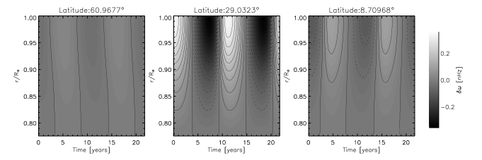
Figure 4: Radial contours of the angular velocity residuals $\delta\omega$ as a function of time at a few selected latitudes for the case shown in Fig. 3. The contours are drawn at intervals of $0.04\,$nHz.

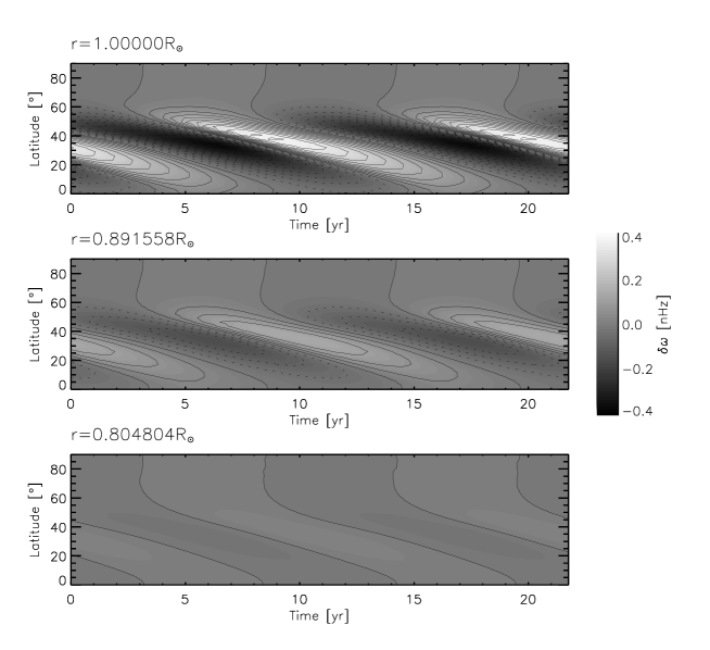
Figure 5: Same as Fig. 3, except that the meridional circulation is not neglected.

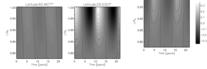
Figure 6: Same as Fig. 4, but the meridional circulation is not neglected.

Figure 7: Variations of the viscosity (solid) and $\partial_{\theta}\omega$ (dashed) with time. Left-hand panel: the case where the meridional circulation is neglected (Fig. 3). Right-hand panel: the case where the meridional circulation is not neglected (Fig. 5).

3 Results

In order to reveal the migrating banded zonal flows, in the following we will plot the distributions of the residual rotation rate, subtracting a temporal average:

$$\delta\omega=\omega-\overline{\omega}$$ (21)

At the bottom of our shell we clearly have $\delta\omega=0$.

First we present the results of a calculation neglecting the meridional flow ($M=C=0$ in equation (2.2)), and using a butterfly diagram with an equatorward branch only ($A_{2}=0$; $\Lambda_{1}>0$). Here we used the radial viscosity profile presented in Fig. 2(a), with $D_{0}=z_{0}=80\,$Mm. Figure 3 shows the evolution of the residual rotation rate $\omega$ as a function of latitude at three different depths.

In order to study the radial behaviour of the zonal flow, we have plotted $\delta\omega$ in Figure 4 as a function of radius and time at a few selected latitudes. It can be seen that the zonal flow pattern penetrates into the convection zone, but the depth of the incursion is only about $0.1R_{\odot}$.

Next, in Figs. 5–6 we consider the effect of switching on the meridional circulation. It is found that the circulation has only a very weak effect on the zonal flow pattern.

Figure 7 present the variations of the viscosity and $\partial_{\theta}\omega$ with time. There is clearly a near phase locking between the shear and the viscosity suppression due to AR.

Figure 8: Amplitude of the residual rotation rate at the surface, at a latitude of $30^{\circ}$ as a function of time. The solid line corresponds to $D_{0}=z_{0}=80\,$Mm and the dashed line to $D_{0}=z_{0}=50\,$Mm. Left-hand panel: using triangular viscosity profile, Fig. 2a. Right-hand panel: using rectangular viscosity profile, Fig. 2b.

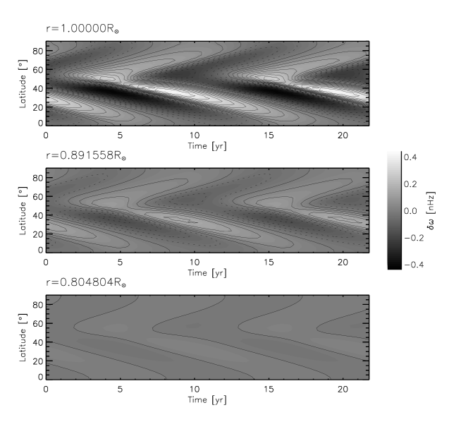
Figure 9: Variation of the residual in rotation rate with latitude and time for a migrating double wave model ($A_{1}/A_{2}=4$, $\Gamma_{1}=-\Gamma_{2}=16$, $\Lambda_{1}=-\Lambda_{2}=4\pi/9$, $\delta_{1}=0$, $\delta_{2}=\pi/4$).

Figure 10: Amplitude of the residual in rotation rate at different latitudes on the surface, as a function of time.

In order to study the influence of the choice of radial profile of the viscosity on the amplitude of the oscillation, we have plotted $\delta\omega$ as a function of time using the different radial profiles of the viscosity in our calculations. (Figure 8). Unsurprisingly, a smaller magnetic tree and/or a faster reduction of the viscosity suppression with depth results in a smaller amplitude of the torsional oscillation. The resulting amplitudes are in general in the range $0.1$–$1\,$nHz, the highest values being comparable to, though still significantly lower than the observed amplitudes. It is the amplitude that shows the greatest sensibility to our model parameters, while the overall shape of the oscillation pattern and its phase relation to the butterfly diagram does not change significantly with the form of the viscosity suppression used.

Finally, Figs. 9–10 show the results for a case where a full, double-wave butterfly diagram is used (Makarov and Sivaraman, 1989). The polar branch, traced by polar faculae, is assumed to be due exclusively to EAR in the present context.

4 Conclusion

We have calculated the spatiotemporal variations of the solar rotation rate in the upper convective zone caused by the suppression of turbulent viscosity due to the presence of magnetic structures associated with (both large and ephemeral) active regions. For concreteness we assumed that these structures can be represented by an assembly of “magnetic trees” with “crown heights” $z_{0}\sim 50$–$80\,$Mm, and that turbulent transport inside these “tree crowns” is effectively absent.

Beside being a simplification, this whole scenario is clearly somewhat speculative, especially as to the subsurface structures corresponding to ephemeral active regions. Nevertheless we believe that this constitutes the best “educated guess” that can be given at present. Still, keeping in mind the uncertainties in the underlying modelling assumptions and in the parameter values of our model, it is important to distinguish between features that seem to be robust and valid for all models of this type from those that are sensible to model details. Apparently robust conclusions that are valid for all the models studied are

• The zonal flows penetrate the convective zone down to a depth of $\sim z_{0}$ only, i.e. to about $0.1\,R_{\odot}$, as shown by observations.

• There is a very good phase coherence between the shear $\partial_{\theta}\omega$ and the viscosity suppression (and therefore the level of activity). We think that this phase relationship is a very important test of models for torsional oscillations. Banded, migrating zonal flows can be produced by a wide variety of models, so such tests are needed to determine which models are compatible with observations also in their details.

• The migration pattern (“butterfly diagram”) of the zonal flows approximately reflects that of the active regions. In particular, if polar faculae are interpreted as a sign of scattered activity in the form of EAR, then a polar branch also arises naturally in the zonal flow migration pattern, as observed. Indeed, our Fig. 9 bears a marked resemblance to Figure 3 in Howe et al. (2001).

On the other hand, one feature of the models that seems to be rather sensitive to details of the model (e.g. triangular vs. rectangular viscosity profiles) and to parameter values (especially $z_{0}$) is the amplitude of the torsional wave. For the cases studied here, the amplitude is in general significantly smaller than the observed amplitude of $\sim 5$–$10\,$nHz. This is true even though for suitable parameter combinations the model can produce amplitudes that can reach a significant fraction of the observed amplitude. For $z_{0}$ values higher than 80 Mm (not shown here) we found that our model can reproduce the full observed amplitude, but at the price of a deeper radial penetration of the zonal flow than observed. Given our present ignorance, one cannot exclude a scenario wherein EAR fields extend down to such great depths, and the shallowness of the torsional oscillations is due to e.g. the prevalence of equatorward angular momentum transport (e.g. $\Lambda$-effect) in the layers below 70 Mm.

Thus, while the overall properties, such as radial dependence and phase, of AR generated torsional oscillations seem to suggest that this mechanism can be partly responsible for the generation of torsional oscillations, the results are not decisive yet.

Further theoretical and observational constraints on the nature of the subsurface magnetic structures associated with both large and ephemeral active regions would be necessary for a better assessment the amplitude of AR-induced zonal flows. Other possible improvements of the present models include the incorporation of this effect in a complete model of differential rotation and angular momentum transport in the convective zone.

Appl. Opt.
K. Petrovay
Eötvös University, Dept. of Astronomy
Budapest, Pf. 32, H-1518 Hungary
E-mail: kris@astro.elte.hu