Interstellar gas in the Galaxy and the X-ray luminosity of Sgr ${\rm A}^{*}$ in the recent past

Information about the X-ray luminosity of the supermassive black hole located at the Galactic center (GC), Sgr ${\rm A}^{*}$, and its temporal variations in the past is imprinted in the scattered emission observed today in the direction towards giant molecular clouds (GMCs) located in our Galaxy. Due to light travel time effects these clouds probe the activity of Sgr ${\rm A}^{*}$ at different times in the past depending on their position relative to the GC and the observer. In this paper we combine results of recent ASCA observations along the Galactic plane, providing upper limits for the scattered flux in the 4-10 keV range produced in a given direction, with data from CO surveys of the same regions. These CO surveys map the position and mass of the molecular gas which the GMCs are made up of. Demanding the scattered flux to be not larger than the observed one, this data enables us to derive upper limits for the 4-10 keV luminosity of Sgr A^∗ at certain times during the last $40\,000$ years down to about $8\times 10^{40}\,{\rm erg\,s}^{-1}$. At other times the limits are less tight, of the order of $10^{41}-10^{42}\,{\rm erg\,s}^{-1}$. For two periods of time of about $2000$ and $4000$ years duration $8000$ and $14\,000$ years ago the currently available CO data is insensitive to any enhanced activity of the GC. Flares lasting longer than 3000 years fill these time gaps and therefore can be excluded to have occured during the last $40\,000$ years with a luminosity larger than a few $10^{42}\,{\rm erg\,s}^{-1}$. The more extended and continuous HI distribution in the Galactic disk, which also scatters the radiation emitted by Sgr A^∗, allows us to extend the time coverage further into the past, back to about $110\,000$ years, albeit the limits are becoming less tight. We thereby can rule out a long term X-ray activity phase of Sgr A^∗ at one per cent of its Eddington level ending less than about $80\,000$ years ago. The limits presented in this paper can be improved by observations of emission in the fluorescent iron K_α-line. We study the feasibility of these methods to investigate past nuclear activity in other spiral galaxies observed with the angular resolution of X-ray telescopes like Chandra and XMM-Newton.

1 Introduction

High spatial resolution observations of the stars in the vicinity of the Galactic center (GC) strongly suggest the presence of a supermassive black hole of mass $2.6\times 10^{6}\,M_{\odot}$ (Genzel et al. 1997; Ghez et al. 1998). Recent Chandra measurements (Baganoff et al. 2001) detect the associated X-ray source Sgr ${\rm A}^{*}$ at a mere $2\times 10^{33}\,{\rm erg}\,{\rm s}^{-1}$, more than ten orders of magnitude below the Eddington luminosity of $3\times 10^{44}\,{\rm erg}\,{\rm s}^{-1}$ for a black hole of this mass. This relative dimness being remarkable in itself raises the question whether Sgr ${\rm A}^{*}$ was equally dim in the past.

Granat spacecraft observations of the region surrounding the GC have revealed a close resemblance between the morphology of the diffuse X-ray emission above 10 keV and the spatial distribution of molecular gas as inferred from CO observations. Sunyaev et al. (1993) proposed that the diffuse, hard X-ray emission observed today in the direction of giant molecular clouds (GMCs) in the central 100 pc of the Galaxy and especially Sgr B2 is radiation emitted by Sgr A^∗ in the past scattered into our line of sight by the molecular gas. They predicted the presence of a strong iron fluorescent K_α-line at $6.4$ keV with an equivalent width of the order of 1 keV. This line is a signature of scattering of hard X-ray photons on neutral matter when the primary photon source does not contribute to the observed emission, by either falling outside of the observing beam or being currently not active (Vainshtein & Sunyaev 1980).

In order for the mass of molecular gas ($\sim 6\times 10^{6}\,M_{\odot}$) present in Sgr B2 to produce the observed flux the X-ray luminosity of Sgr A^∗ must have been of the order of $2\times 10^{39}{\rm erg\,s}^{-1}$ about 400 years ago. This time delay corresponds to the different path lengths for photons received directly or taking the detour via Sgr B2, which lies at a projected distance of $\sim 120$ pc from the GC.

Evidence for the scattering scenario has been discovered with the spectroscopic imaging capabilities of the ASCA satellite (Koyama et al. 1996; Sunyaev et al. 1998; Murakami et al. 2000). The X-ray spectrum of Sgr B2 exhibits strong emission in the iron K_α-line at $6.4$ keV confirming the prediction of Sunyaev et al. (1993). Murakami et al. (2001A) have recently observed another GMC close to the GC, Sgr C, to be bright in the K_α-line, strengthening the case for the scattering scenario. Theses authors call Sgr B2 and Sgr C “X-ray reflection nebulae”. Recent Chandra observations (Murakami et al. 2001B) confirm the ASCA results about Sgr B2 and the nature of the 6.4 keV K_α-line emission.

The application of the method successfully used in the above described cases to constrain the luminosity of Sgr A^∗ in the past is not restricted to GMCs close to the GC. For it to provide nontrivial constraints upon the strength of the activity of the GC one needs a scattering material with a sufficient optical depth and an estimate of the scattered flux produced by this material. In the case of our Galaxy two obvious choices which fulfill these criteria are interstellar molecular and atomic hydrogen:

• CO surveys covering the Galactic plane have shown that about $10^{9}\,M_{\odot}$ of H₂ reside in GMCs on orbits between the GC and the sun with a peak mass surface density around a galactocentric radius between $4$ and $6$ kpc, the so called molecular ring (e. g. Dame 1993). The time delays, the difference of the arrival times between the primary and the scattered radiation, for clouds located in the molecular ring range up to about $40\,000$ years.

  In this paper we will compute the scattered flux produced by a GMC in response to a strong flare of Sgr ${\rm A}^{*}$. This flux is detectable by current X-ray telescopes even if it was relatively short, with a duration of the order of years. Turning this argument around one infers from the observed relative dimness of GMCs today that there could not have been a strong flare of Sgr ${\rm A}^{*}$ at those times in the past, which correspond to the time delays of massive GMCs in our Galaxy.

  The good temporal “resolution” with an uncertainty of the occurrence of a flare of the order of years comes about because the mass of a GMC is rather concentrated with a very dense core. We are therefore in principle able to pinpoint past flares of Sgr ${\rm A}^{*}$ during the last $40\,000$ years very well if there exists a GMC with a corresponding time delay.

  The drawback of this “accurate” timing is that because there only exist a finite number of GMCs in our Galaxy it is not possible to cover the whole time interval from $40\,000$ years ago, the time delay of the most distant clouds, until “today”. For the analysis presented in this paper it was only possible to use the CO data from the first Galactic quadrant. This means that we are missing all the GMCs, which are located in the fourth Galactic quadrant and which should be equally numerous. This additional data would probably improve the “filling factor” of our sample but still leave several time gaps and not extend the time coverage beyond $40\,000$ years. The possibility thus always exists that a short flare of Sgr A^∗ occured during the last $40\,000$ years unnoticed by us, because there is no GMC which could respond to this flare. If we take only the available CO data into account the coverage becomes complete for flares longer than about 3000 years and we can thereby rule out any flare brighter than a few $10^{42}\,{\rm erg}\,{\rm s}^{-1}$ during the last $40\,000$ years of this or a longer duration.

• The HI phase of the interstellar medium (ISM) is more diffusely distributed than H₂. It extends out to about 16 kpc with an approximately constant mass surface density of about $4\,M_{\odot}\,{\rm pc}^{-2}$, corresponding to a total mass of the order of $3\times 10^{9}\,M_{\odot}$ (e. g. Dame 1993). This implies that the total mass of neutral hydrogen in a field of view of the ASCA instrument is larger than the mass of any GMC even those near the GC. For a Galactic longitude of $10^{\mathrm{o}}$ it is about $2\times 10^{7}\,M_{\odot}$.

  Due to its more continuous distribution the response of the HI distribution to flares of Sgr A^∗ will be spread out over a long time interval. Therefore we are unable to locate the time when a flare happened. A strong flare longer ago can produce the same response as a weak flare not so long ago. Nevertheless due to the larger extent of HI in the Galactic disk we can extend the time coverage back to about $110\,000$ years. We will show that for example the switch off case from $1\%$ of the Eddington luminosity of Sgr A^∗ (the whole Galactic disk is illuminated by Sgr A^∗, which suddenly “switches off” at a time $t_{\mathrm{o}}$) can be ruled out to have ended less than about $80\,000$ years ago.

The ASCA Galactic Plane Survey (Sugizaki et al. 2001), provides upper limits for the diffuse X-ray emission produced by scattering along certain directions. In this paper we compute the expected scattered flux for an assumed Eddington luminosity of $3\times 10^{44}\,{\rm erg}\,{\rm s}^{-1}$ in the 4-10 keV range. Although this value is rather large the results can be rescaled to any input luminosity because the problem is linear. It is obvious that the ratio of the computed scattered flux to the upper limit for the scattered flux given by ASCA observations, $f=F_{\mathrm{sc}}/F_{\mathrm{obs}}$, gives us an estimate of the average luminosity of the GC, $L_{\mathrm{GC}}\mathchoice{\mathrel{\vbox{\hbox{$\buildrel\displaystyle<\over{\displaystyle\sim}$}}}}{\mathrel{\vbox{\hbox{$\buildrel\textstyle<\over{\textstyle\sim}$}}}}{\mathrel{\vbox{\hbox{$\buildrel\scriptstyle<\over{\scriptstyle\sim}$}}}}{\mathrel{\vbox{\hbox{$\buildrel\scriptscriptstyle<\over{\scriptscriptstyle\sim}$}}}}f^{-1}L_{\mathrm{Edd}}$, at a time which corresponds to the time delay of the observed GMC.

This paper is structured as follows. In the following section we recall the basic ideas and relations of X-ray archaeology. We describe how we extracted the CO and X-ray data necessary for our purposes from the literature. In Sec. 3 we will derive constraints for the past X-ray luminosity of Sgr ${\rm A}^{*}$ using a sample of GMCs in the Galaxy. In Sec. 4 we will describe the limits the Galactic HI distribution can provide. The possibility to use the same methods to study past nuclear activity in other spiral galaxies is studied in Sec. 5. In Sec. 6 we close with a discussion of our results.

2 Method

Figure 1: A sketch of the scenario studied projected onto the Galactic plane. A time $t_{\mathrm{o}}$ ago the luminosity of Sgr A^∗ (marked by a cross) flared. This enhanced activity lasted for a period $\Delta$. Relative to the earth bound observer (small circle), observing at a time t and orbiting Sgr A^∗ on the dotted circle, the GMCs that lie between the two ellipsoids corresponding to the beginning and the end of the flare are exposed to this enhanced emission. For other GMCs the period of enhanced irradiation already has passed or has not started yet. The boundaries of an observational field of view are sketched by dashed lines. Inside this field of view one cloud has already faded and another one is partially covered by the flare. Two possible photon paths between Sgr A^∗ and the observer are marked by dot-dashed lines (one of them covered half way by the z-axis). The ellipsoids are rotationally symmetric about the z-axis.

2.1 X-ray Archaeology

The scenario we have in mind is sketched in Fig. 1. An outburst of duration $\Delta$ has occured at the GC a time $t_{\mathrm{o}}$ ago, as measured by the earth bound observer. As time evolves this signal moves radially outwards from the GC and starts illuminating GMCs at larger and larger galactocentric distances. These clouds scatter a fraction of the incident radiation into the direction of the observer.

The loci of scattering sites giving a fixed time delay form an ellipsoid with foci at the source and the observer. Since the system is symmetric around the line connecting the GC and the observer this ellipsoid is fully described by two parameters which depend upon time past since the detection of the burst $t-t_{\mathrm{o}}$, where $t$ is the time of observation. In this section we will assume from now on $t_{\mathrm{o}}=0$ to simplify the following formulae.

Choosing a cartesian coordinate system (see Fig. 1) with the GC and the Sun at $z=R_{\mathrm{o}}/2$ and $z=-R_{\mathrm{o}}/2$ respectively, the ellipsoid can be expressed as

$$\frac{z^{2}}{a^{2}}+\frac{x^{2}+y^{2}}{b^{2}}=1,$$ (1)

where the lengths of the major and minor axis are $a=(ct+R_{\mathrm{o}})/2$ and $b=\sqrt{(ct)^{2}+2ctR_{\mathrm{o}}}/2$, with $c$ the speed of light and $R_{\mathrm{o}}$ the distance to the GC.

An alternative description of the ellipsoid can be given in polar coordinates $R$, $\phi$ (defined in Fig. 1):

$$R(\phi)=\frac{p}{1+e\cos\phi},$$ (2)

with $p=b^{2}/a$ and $e=R_{\mathrm{o}}/(2a)$. Note that in the limit of the observer at infinity $(R_{\mathrm{o}}\rightarrow\infty,p\rightarrow ct,e\rightarrow 1)$ this ellipsoid becomes a paraboloid

$$R(\phi)=\frac{ct}{1+\cos\phi}.$$ (3)

This approximation is valid for GMCs at the GC ($R_{\mathrm{o}}\gg ct$) and has been studied in the context of Sgr B2 by Sunyaev & Churazov (1998). In cartesian coordinates the paraboloid is described by:

$$z=\frac{1}{2}\left(ct-\frac{x^{2}+y^{2}}{ct}\right)+\frac{R_{\mathrm{o}}}{2}.$$ (4)

The velocities of the surfaces of constant time delay along the major and minor axes of the ellipsoid are obtained by differentiation of the formulae for a and b. The major axis increases at a constant speed of $c/2$. The velocity along the minor axes depends upon time as follows

$$\dot{b}=\frac{c}{2}\frac{ct+R_{\mathrm{o}}}{\sqrt{(ct)^{2}+2ctR_{\mathrm{o}}}}.$$ (5)

At times small compared to $R_{\mathrm{o}}/c$ this velocity is larger than the velocity of light and approaches the value $c/2$ for $ct\gg R_{\mathrm{o}}$. Inside the Galaxy, where most of the GMCs lie inside the solar circle ($R<R_{\mathrm{o}}$), this velocity is always larger than $(2/\sqrt{3})(c/2)\approx 0.58c$.

The velocity in a general direction $\phi$ is given by the temporal derivative of Eq. 2 which yields

$$\dot{R}(\phi)=\frac{c}{2}\,\frac{c^{2}t^{2}+2R_{\mathrm{o}}(ct+R_{\mathrm{o}})(1+\cos\phi)}{(ct+R_{\mathrm{o}}(1+\cos\phi))^{2}}.$$ (6)

In the paraboloid approximation this becomes, by either differentiating Eq. 3 with respect to $t$ or by taking the limit $R_{\mathrm{o}}\gg ct$ of Eq. 6,

$$\dot{R}(\phi)=\frac{c}{1+\cos\phi}.$$ (7)

The apparent velocity is given by the projection onto the plane of the sky, which reads

$$v_{\mathrm{app}}=\frac{c\sin\phi}{1+\cos\phi}.$$ (8)

This equation is equivalent to the formula for apparent superluminal motion of matter having velocities close to the speed of light, which is normally expressed in terms of the angle $\theta=\pi-\phi$. The formula for the apparent velocity in the Galactic plane in the ellipsoid case is given by

$$v_{\mathrm{app}}=\frac{c}{2}\,\frac{c^{2}t^{2}+2R_{\mathrm{o}}(ct+R_{\mathrm{o}})(1+\cos\phi)}{(ct+R_{\mathrm{o}}(1+\cos\phi))^{2}}\,\sin(\phi-l).$$ (9)

One obtains an additional dependence upon $l$, because the projection angle for a given direction $\phi$ depends upon galactocentric distance $R$ and therefore upon time.

The average time delay of photons scattered by a cloud with galactocentric radius $R$ and distance from the observer $d$ is given by:

$$\delta=(R+d-R_{\mathrm{o}})/c.$$ (10)

It is obvious that for clouds with a constant galactocentric distance $R$ those, which lie behind the GC, produce the largest time delay $\delta_{\mathrm{max}}(R={\rm const.})=2R/c$. For clouds with a distance of 6 kpc to the GC, the edge of the molecular ring, the largest time delay is about $40\,000$ years. The more diffuse HI phase of the interstellar medium (ISM) extends up to radii of about 16 kpc (Dame 1993). Matter at these distances can in principle probe the activity of the GC about $110\,000$ years ago.

2.2 GMCs in the Galactic disk

Figure 2: The spatial distribution of GMCs selected from SRBY87 for this work. The GMCs cover a range of Galactic longitudes of $8^{\mathrm{o}}\leq l\leq 60^{\mathrm{o}}$. The position of the GC is marked by a cross. The position of the sun (marked by a small circle) is at coordinates $(-8.5,0.0)$. For Galactic longitudes covered by ASCA observations the solar circle is marked by solid arcs. For Galactic longitudes falling outside of the ASCA survey the solar circle is marked by a dotted line. The different symbols denote different cloud masses: $M_{\mathrm{cl}}\leq 5\times 10^{5}\,M_{\odot}$ (diamonds), $5\times 10^{5}\,M_{\odot}<M_{\mathrm{cl}}\leq 10^{6}\,M_{\odot}$ (triangles) and $M_{\mathrm{cl}}>10^{6}\,M_{\odot}$ (squares).

The results of several CO surveys have been published over the last decades. They map the CO brightness temperature as a function of Galactic longitude $l$, Galactic latitude $b$ and radial velocity component $v_{r}$, differing in resolution and area surveyed.

Solomon et al. (1987, SRBY87) have published a list (see Table 1 in their paper) of 273 molecular clouds detected with the Massachusetts-Stony Brook CO Galactic Plane Survey of the first Galactic quadrant. These clouds were extracted from the three dimensional $(l,b,v_{r})$ data cube by locating surfaces of equal brightness temperature. The distances were computed from the radial velocity component of the centroids under the usual assumption (see e.g. Binney & Merrifield 1998) that clouds move on circular orbits with a constant circular velocity of $\Theta_{\mathrm{o}}=220\,{\rm km\,s}^{-1}$.

The assumption of circular orbits with a constant rotational velocity is a fair approximation for clouds inside of the solar circle but breaks down at small galactocentric radii because the orbits are probably highly non circular in this region. For GMCs inside the solar circle a ambiguity is inherent to this method of distance determination. A cloud with a given measured radial velocity component can either lie on the near or the far side of the circular orbit it is assumed to travel around the GC. SRBY87 were able to overcome this ambiguity by several methods described in their paper.

GMC	$l$/deg	$b$/deg	$R$/kpc	$d$/kpc	$\delta^{\mathrm{a}}$	$M_{\mathrm{cl}}^{\mathrm{b}}$	$r_{\mathrm{cl}}$/pc	$t_{\mathrm{cl}}^{\mathrm{a}}$	$F_{\mathrm{sc}}^{\mathrm{c}}$	$F_{\mathrm{obs}}^{\mathrm{d}}$	$L_{\mathrm{GC}}^{\mathrm{e}}$
003	08.30	+0.00	3.4	5.3	669	55.6	19.3	44	$7.1\times 10^{-8}$	$1.9\times 10^{-11}$	$8.0\times 10^{40}$
014	10.00	-0.04	4.6	4.0	335	11.3	5.8	12	$1.2\times 10^{-8}$	$1.5\times 10^{-11}$	$3.8\times 10^{41}$
059	17.20	-0.20	5.2	12.7	31449	199.1	29.7	353	$9.4\times 10^{-9}$	$1.7\times 10^{-11}$	$5.4\times 10^{41}$
080	20.75	+0.10	4.2	5.1	2677	21.6	8.9	39	$1.0\times 10^{-8}$	$1.5\times 10^{-11}$	$4.5\times 10^{41}$
085	21.75	+0.00	4.6	4.5	2007	36.4	9.4	37	$1.6\times 10^{-8}$	$1.6\times 10^{-11}$	$3.0\times 10^{41}$
089	22.05	+0.20	5.4	3.6	1673	33.7	11.9	38	$2.5\times 10^{-8}$	$1.6\times 10^{-11}$	$1.9\times 10^{41}$
116	24.60	-0.15	4.4	10.3	20743	106.7	13.4	126	$5.2\times 10^{-9}$	$1.5\times 10^{-11}$	$8.7\times 10^{41}$
122	25.65	-0.10	4.2	9.8	18401	202.6	28.2	283	$1.7\times 10^{-8}$	$1.8\times 10^{-11}$	$3.2\times 10^{41}$
128	25.90	-0.15	3.8	7.7	10037	107.5	17.2	133	$1.2\times 10^{-8}$	$1.7\times 10^{-11}$	$4.3\times 10^{41}$
151	28.30	-0.10	4.8	4.9	4015	41.7	12.5	54	$1.3\times 10^{-8}$	$1.4\times 10^{-11}$	$3.2\times 10^{41}$
152	28.60	+0.05	4.3	7.5	11041	63.3	11.7	90	$5.4\times 10^{-9}$	$1.4\times 10^{-11}$	$7.8\times 10^{41}$
158	29.00	+0.05	4.3	7.5	11041	48.9	18.0	145	$6.4\times 10^{-9}$	$1.5\times 10^{-11}$	$7.0\times 10^{41}$
162	29.85	-0.05	4.3	7.4	10706	85.1	15.8	127	$8.5\times 10^{-9}$	$1.5\times 10^{-11}$	$5.3\times 10^{41}$
171	30.80	-0.05	4.6	5.8	6357	119.3	22.1	107	$2.3\times 10^{-8}$	$1.3\times 10^{-11}$	$1.7\times 10^{41}$
191	33.90	+0.10	4.8	7.1	11375	54.8	15.6	119	$6.0\times 10^{-9}$	$1.0\times 10^{-11}$	$5.0\times 10^{41}$
193	34.25	+0.10	6.1	3.1	2342	39.4	9.3	42	$1.6\times 10^{-8}$	$1.0\times 10^{-11}$	$1.9\times 10^{41}$
201	35.20	-0.10	7.9	0.8	669	2.0	3.4	18	$1.6\times 10^{-8}$	$9.1\times 10^{-12}$	$1.7\times 10^{41}$
206	36.40	-0.10	6.3	3.1	3011	23.2	8.8	42	$1.1\times 10^{-8}$	$1.0\times 10^{-11}$	$2.7\times 10^{41}$
214	39.85	-0.20	6.3	9.6	24758	375.3	47.4	469	$1.6\times 10^{-8}$	$7.7\times 10^{-12}$	$1.4\times 10^{41}$
217	41.15	-0.20	6.2	9.1	22750	201.2	22.4	215	$6.7\times 10^{-9}$	$8.6\times 10^{-12}$	$3.9\times 10^{41}$

• Time delay $\delta$ and time for the ellipsoid to cross the cloud $t_{\mathrm{cl}}$ in units of years

• Mass of cloud in units of $10^{4}\,M_{\odot}$

• Scattered flux in the 4-10 keV range in units of ${\rm erg}\,{\rm cm}^{-2}\,{\rm s}^{-1}$ for the whole cloud covered by a flare

• Flux in the 4-10 keV range observed by ASCA in units of ${\rm erg}\,{\rm cm}^{-2}\,{\rm s}^{-1}$

• Upper limit for the luminosity of Sgr A^∗ in the 4-10 keV range in units of ${\rm erg}\,{\rm s}^{-1}$ a time $\delta$ ago

Table 1: Selected parameters (number of cloud in SRBY87 sample, Galactic longitude, Galactic latitude, galactocentric distance, distance, time delay, mass, radius, time for ellipsoid to cross the cloud, scattered flux, observed flux and upper limit for the luminosity of Sgr A^∗) of twenty GMCs from our sample.

This data set is not the most recent one (for more recent surveys of this area see, e.g. Dame et al. (2001) and Lee et al. (2001)) but to our knowledge up to today the only one where mass estimates of a large number of individual GMCs have been presented.

Not all of the clouds listed in SRBY87 fall into one of the fields of view of the ASCA Galactic Plane Survey. These are clouds located at longitudes larger than $60^{\mathrm{o}}$ or at latitudes larger than $0.3^{\mathrm{o}}$. Combining the two data sets leaves one with 96 clouds out of 273. The spatial distribution of these clouds in the Galactic plane is plotted in Fig. 2, symbolised according to their mass (for the distribution of the full set of clouds see Solomon & Rivolo 1989). Although spiral structure might be marginally discernible in this picture, the concentration of GMCs along the molecular ring is clearly visible.

The cloud properties needed for this work are the Galactic longitude $l$, the galactocentric radius $R$, the distance from the observer $d$, the radius $r_{\mathrm{cl}}$ and the mass $M_{\mathrm{cl}}$ of a cloud, which was computed with the observed velocity dispersion and should thus not be affected by recalibrations of the I(CO)/N(H₂) ratio. For the subsample of clouds we are working with these parameters fall in the ranges $1.9\times 10^{4}\,M_{\odot}\mathchoice{\mathrel{\vbox{\hbox{$\buildrel\displaystyle<\over{\displaystyle\sim}$}}}}{\mathrel{\vbox{\hbox{$\buildrel\textstyle<\over{\textstyle\sim}$}}}}{\mathrel{\vbox{\hbox{$\buildrel\scriptstyle<\over{\scriptstyle\sim}$}}}}{\mathrel{\vbox{\hbox{$\buildrel\scriptscriptstyle<\over{\scriptscriptstyle\sim}$}}}}M_{\mathrm{cl}}\mathchoice{\mathrel{\vbox{\hbox{$\buildrel\displaystyle<\over{\displaystyle\sim}$}}}}{\mathrel{\vbox{\hbox{$\buildrel\textstyle<\over{\textstyle\sim}$}}}}{\mathrel{\vbox{\hbox{$\buildrel\scriptstyle<\over{\scriptstyle\sim}$}}}}{\mathrel{\vbox{\hbox{$\buildrel\scriptscriptstyle<\over{\scriptscriptstyle\sim}$}}}}3.8\times 10^{6}\,M_{\odot}$, $2.5\mathchoice{\mathrel{\vbox{\hbox{$\buildrel\displaystyle<\over{\displaystyle\sim}$}}}}{\mathrel{\vbox{\hbox{$\buildrel\textstyle<\over{\textstyle\sim}$}}}}{\mathrel{\vbox{\hbox{$\buildrel\scriptstyle<\over{\scriptstyle\sim}$}}}}{\mathrel{\vbox{\hbox{$\buildrel\scriptscriptstyle<\over{\scriptscriptstyle\sim}$}}}}r_{\mathrm{cl}}\mathchoice{\mathrel{\vbox{\hbox{$\buildrel\displaystyle<\over{\displaystyle\sim}$}}}}{\mathrel{\vbox{\hbox{$\buildrel\textstyle<\over{\textstyle\sim}$}}}}{\mathrel{\vbox{\hbox{$\buildrel\scriptstyle<\over{\scriptstyle\sim}$}}}}{\mathrel{\vbox{\hbox{$\buildrel\scriptscriptstyle<\over{\scriptscriptstyle\sim}$}}}}47$ pc and $3\times 10^{2}{\rm years}\mathchoice{\mathrel{\vbox{\hbox{$\buildrel\displaystyle<\over{\displaystyle\sim}$}}}}{\mathrel{\vbox{\hbox{$\buildrel\textstyle<\over{\textstyle\sim}$}}}}{\mathrel{\vbox{\hbox{$\buildrel\scriptstyle<\over{\scriptstyle\sim}$}}}}{\mathrel{\vbox{\hbox{$\buildrel\scriptscriptstyle<\over{\scriptscriptstyle\sim}$}}}}\delta\mathchoice{\mathrel{\vbox{\hbox{$\buildrel\displaystyle<\over{\displaystyle\sim}$}}}}{\mathrel{\vbox{\hbox{$\buildrel\textstyle<\over{\textstyle\sim}$}}}}{\mathrel{\vbox{\hbox{$\buildrel\scriptstyle<\over{\scriptstyle\sim}$}}}}{\mathrel{\vbox{\hbox{$\buildrel\scriptscriptstyle<\over{\scriptscriptstyle\sim}$}}}}4\times 10^{4}{\rm years}$. Note that in SRBY87 a distance of the sun to the GC of 10 kpc was assumed. We have rescaled the distances and derived cloud properties to $R_{\mathrm{o}}=8.5\,{\rm kpc}$. In Table 1 (columns 1-8) we list the important parameters for twenty clouds out of our sample. Note that the GMCs in SRBY87 have been ordered and numbered according to their Galactic longitude.

2.3 Scattered flux

The ASCA observations of the Galactic plane $(b\approx 0^{\mathrm{o}})$ in the longitude range $-45^{\mathrm{o}}\leq l\leq 63^{\mathrm{o}}$ have been compiled and analysed by Sugizaki et al. (2001). In Fig. 2 we have tried to illustrate the range of longitudes covered by the ASCA Galactic Plane Survey by plotting solid arcs at a distance $R_{\mathrm{o}}$ from the GC, where observations have been made. It is obvious that we are missing the CO data from the fourth Galactic quadrant. As mentioned before surveys of this area exist (e. g. Dame et al. 2001) but to our knowledge this data has not yet been fully analysed. The distribution of GMCs should be symmetric between the Galactic quadrants I and IV. We should therefore expect a similar number of GMCs in the fourth Galactic quadrant.

The ASCA observations have been presented in three energy bands. Most interesting for this work because least affected by photoelectric absorption is the X-ray surface brightness in the hardest, the 4-10 keV, spectral band. The corresponding fluxes at all longitudes are all of a similar order of magnitude. Not even one cloud seems to be especially bright “at the moment”.

Even if the diffuse X-ray flux observed in one field of view originates from a different physical process than scattering, it is still an upper limit for the flux produced through scattering by gas distributed along this beam: $F_{\mathrm{sc}}\leq F_{\mathrm{obs}}$.

The clouds in our sample have optical depths for Thomson scattering up to $\tau_{\mathrm{T}}\approx 10^{-1}$. We therefore consider scattering in the optically thin limit. Our treatment of absorption is described in Sec. 2. 3. 1. Nearly the whole Galaxy is transparent to X-rays with energies above 4 keV, except some regions around the GC. But even here optically thick GMCs do not shield the whole disk of the Galaxy from the illumination by Sgr A^∗. The covering fraction is probably rather small.

In the optically thin case the scattered surface brightness in a given direction at energy $E$ and time of observation $t$ is given by

$$I_{\mathrm{sc}}(E,t)=\int_{s_{\mathrm{min}}(t)}^{s_{\mathrm{max}}(t)}n(s)\frac{L_{\mathrm{GC}}(E,t_{\mathrm{ret}})}{4\pi R(s)^{2}}\left(\frac{{\rm d}\sigma}{{\rm d}\Omega}\right){\rm d}s,$$ (11)

where $s_{\mathrm{min}}$ and $s_{\mathrm{max}}$ are the boundaries of integration, $n(s)$ is the number density of the scattering gas at a distance $s$ from the observer, $t_{\mathrm{ret}}=t-(R(s)+s)/c$ the “retarded” time, $R$ the distance to the GC and $({\rm d}\sigma/{\rm d}\Omega)$ the differential scattering cross-section. The time dependent integration limits are the points of intersection of the line of sight with the ellipsoids corresponding to the beginning and the end of a flare.

The scattered flux is given by the integration of the surface brightness over the field of view of the ASCA instrument. We take into account the cases when parts of a cloud fall outside the field of view, as sketched in Fig. 1, or when the field of view is larger than a cloud:

$$F_{\mathrm{sc}}(E,t)=\int I_{\mathrm{sc}}(E,t){\rm d}\Omega.$$ (12)

We neglect here the iron K_α-line production and the corresponding iron K-edge absorption. The detailed ASCA spectral data are not yet publicly available. XMM-Newton will provide much improved data including K_α-line limits, which will improve the limits for the X-ray luminosity of Sgr A^∗ derived in the following sections.

In the optical thin case the scattered luminosity is proportional to the mass of the illuminated scattering material. An order of magnitude estimate of the above integrals to demonstrate the scaling yields

$$L_{\mathrm{sc}}\sim\frac{3}{16\pi}\frac{\sigma_{\mathrm{T}}}{R^{2}}\frac{M_{\mathrm{cl}}}{m_{\mathrm{p}}}L_{\mathrm{GC}}.$$ (13)

This formula neglects the spatial extension of the scattering gas and the angular dependence of the differential scattering cross-section and assumes that the whole cloud is covered by the flare, implying that all of the mass contributes to the scattered emission. For typical cloud parameters one obtains a scattered luminosity of

$$L_{\mathrm{sc}}\sim 6\times 10^{37}\,{\rm erg\,s}^{-1}\left(\frac{L_{\mathrm{GC}}}{L_{\mathrm{Edd}}}\right)\left(\frac{M_{\mathrm{cl}}}{10^{6}\,M_{\odot}}\right)\left(\frac{5\,{\rm kpc}}{R}\right)^{2},$$ (14)

which for $L_{\mathrm{GC}}\sim L_{\mathrm{Edd}}$ is comparable to the luminosity of the brightest X-ray binaries in the Galaxy, thereby certainly contradicting the observations.

If the flare duration $\Delta$ is shorter than the time for the ellipsoid to sweep across the cloud one has to multiply Eq. 14 by an additional factor

$$\left(\frac{\Delta}{2r_{\mathrm{cl}}/v_{\mathrm{ell}}}\right),$$ (15)

where $v_{\mathrm{ell}}$ is the velocity of the ellipsoid across the cloud, which can be superluminal depending on the relative orientation of the cloud with respect to the GC and the observer. This additional factor takes into account that only a fraction $\sim\Delta/(2r_{\mathrm{cl}}/v_{\mathrm{ell}})$ of the mass of the cloud is illuminated.

2.3.1 Absorption

As X-ray photons of energy $E$ traverse the ISM a fraction $\tau_{\mathrm{ph}}(E)$ of them is absorbed by the heavy elements of the interstellar gas, again assuming optically thin conditions. Therefore a GMC will be exposed to a flux $(L_{\mathrm{gc}}(E,t_{\mathrm{ret}})/4\pi R^{2})\exp[-\tau_{\mathrm{ph}}^{\prime}(E)]$, where $\tau_{\mathrm{ph}}^{\prime}(E)$ is the optical depth for photoelectric absorption at energy $E$ between the GC and the GMC. The observer will measure a flux $F_{\mathrm{sc}}(E,t)\exp[-\tau_{\mathrm{ph}}(E)]$. The optical depth due to photoelectric absorption is proportional to the hydrogen column density $N_{\mathrm{H}}$

$$\tau_{\mathrm{ph}}(E)=N_{\mathrm{H}}\sigma_{\mathrm{ph}}(E),$$ (16)

where $\sigma_{\mathrm{ph}}(E)$ is the photoelectric absorption cross-section per hydrogen atom, which we compute with an analytic fit by Morrison & McCammon (1983).

We estimate $N_{\mathrm{H}}$ with the average mass surface density of a GMC given by $\Sigma_{\mathrm{cl}}\approx M_{\mathrm{cl}}/r_{\mathrm{cl}}^{2}\pi$, which leads to $N_{\mathrm{H}}\approx(3/4)(\Sigma_{\mathrm{cl}}/m_{\mathrm{p}})$. Since we have no better knowledge about the hydrogen column density between the GC and a cloud, we furthermore assume $N_{\mathrm{H}}^{\prime}=N_{\mathrm{H}}$.

2.3.2 Differential scattering cross-section for a mixture of H₂ and He

Figure 3: The scattered flux in the 4-10 keV as a function of the angle $\alpha$ (defined in Fig. 1) for a cloud of $10^{6}\,M_{\odot}$ at 5 kpc distance from the GC and the observer fully illuminated by an Eddington flare of Sgr A^∗. Note that $\alpha=\pi$ corresponds to the case of forward scattering. The lines mark different mass compositions of the cloud: 70% H₂ + 30% He (solid line), atomic hydrogen (dashed) and molecular hydrogen (dotted).

In the following sections we will assume that the GMCs in our sample are composed of 70% molecular hydrogen and 30% helium. It is known (e. g. Sunyaev & Churazov 1996) that in the energy range considered scattering by the bound electrons of molecular hydrogen and helium is important, because for small scattering angles the differential scattering cross-section per electron for Rayleigh scattering on molecular hydrogen and helium can become two times larger than the one for hydrogen atoms, which at these energies is identical to the Thomson differential cross-section. The angular dependence for Thomson scattering is proportional to $(1+\cos^{2}\theta_{\mathrm{sc}})$, where $\theta_{\mathrm{sc}}$ is the scattering angle of the photon, which is approximately given by the angle $\alpha$ defined in Fig. 1.

In Fig. 3 we plot the scattered flux for a single cloud of $10^{6}\,M_{\odot}$ composed of pure molecular hydrogen, a mixture of 70% molecular hydrogen and 30% helium and pure atomic hydrogen as a function of the angle $\alpha$ ($\alpha=\pi$ corresponds to the case of forward scattering). We chose a galactocentric distance and a distance to the observer of 5 kpc. We used the differential scattering cross-section for scattering by atomic, molecular hydrogen and helium as a function of photon energy and scattering angle as presented in Sunyaev et al. (1999).

The scattered flux for the compositions including molecular hydrogen are larger than the one for atomic hydrogen because for small scattering angles ($\alpha\mathchoice{\mathrel{\vbox{\hbox{$\buildrel\displaystyle<\over{\displaystyle\sim}$}}}}{\mathrel{\vbox{\hbox{$\buildrel\textstyle<\over{\textstyle\sim}$}}}}{\mathrel{\vbox{\hbox{$\buildrel\scriptstyle<\over{\scriptstyle\sim}$}}}}{\mathrel{\vbox{\hbox{$\buildrel\scriptscriptstyle<\over{\scriptscriptstyle\sim}$}}}}\pi$) the two electrons present in molecular hydrogen and helium scatter coherently. The scattered flux for the chosen mixture of molecular hydrogen and helium is smaller than the one for pure molecular hydrogen because in this case there are only .85 electrons per nucleon compared to 1 electron per nucleon for pure hydrogen, atomic or molecular.

3 Limits on the X-ray luminosity of Sgr A^∗ from Giant Molecular Clouds

There exist several characteristic variability timescales for a supermassive black hole such as Sgr A^∗. The shortest possible timescale is related to the linear size of the region, where the bulk of energy is released in the accretion disk around a black hole (Shakura & Sunyaev 1973): $t_{\mathrm{bh}}\sim 10R_{\mathrm{g}}/c\sim 300\,{\rm s}$ for Sgr A^∗, where $R_{\mathrm{g}}$ is the Schwarzschild radius of the black hole. Tidal disruption events are believed to produce an Eddington level flare over a period $t_{\mathrm{tidal}}\sim{\rm years}$ (Rees 1988). The lifetimes of active galactic nuclei (AGN) are believed to be of the order of $10^{7}-10^{8}$ years. The detailed temporal evolution of the luminosity of Sgr A^∗ is probably rather complex, possibly varying on all of the above timescales.

In this study it is our aim to constrain the past luminosity of Sgr A^∗ from information about the reprocessing system, the spatially distributed GMCs in the Galactic disk, and the output signal at one point in time, the scattered flux observed today. This is reminiscent of the methods used in reverberation mapping in AGN (see e. g. Peterson 1993). There one tries to gain information about the geometry and kinematics of the emission-line region (the reprocessing system) by monitoring the continuum variations (the input) and the resulting emission-line response (the output). Mathematically this is described by a transfer function, which applied to our problem can be written as:

$$F_{\mathrm{sc}}(t)=\int_{-\infty}^{\infty}\Psi(t^{\prime})L_{\mathrm{GC}}(t-t^{\prime})\,{\rm d}t^{\prime}$$ (17)

The scattered flux observed at a time t is the response of our system to activity of the GC in the past. In reverberation mapping in AGN one determines the transfer function using Fourier transforms of the input and the output over a certain period of time. In our case this is not possible because the scattered flux or its upper limit is known only at one moment in time.

If the cloud had no spatial extension, a “point mass”, the transfer function would be just a $\delta$-function with an amplitude proportional to the mass of the cloud. The transfer function for several clouds with different time delays would be a sum of $\delta$-functions. In these cases it would be possible to ascribe an unique X-ray luminosity of Sgr A^∗ to an observed scattered flux.

Due to the spatial extension of a GMC with an internal density distribution this $\delta$-function is smeared out in time. This means that the scattered flux observed at one moment in time depends upon the luminosity of the GC over a certain period of time in the past. The correspondence between the observed scattered flux and the luminosity of the GC is therefore not one to one anymore.

What one can do in this case to constrain the luminosity of Sgr A^∗ is to assume some input, a “test function”, and compare the resulting output with the observations. Should the output be inconsistent with the observed flux then the initial input must be wrong.

We assume the temporal and spectral behaviour of the luminosity of Sgr A^∗ to be of the following form

$$L_{\mathrm{GC}}(E,t)=\cases{L_{\mathrm{o}}(E_{\mathrm{o}}/E)&$t_{\mathrm{on}}$ $\leq$ $t$ $\leq$ $t_{\mathrm{off}}$\cr 0&$\mathrm{else,}$\cr}$$ (18)

with $t_{\mathrm{on}}=t_{\mathrm{o}}-\Delta/2$ and $t_{\mathrm{off}}=t_{\mathrm{o}}+\Delta/2$. The choice of the spectral behaviour implies a photon index of 2, which is representative of observed AGN spectra in the 4-10 keV range. Note that here we define for the sake of symmetry $t_{\mathrm{o}}$ as the time half way through the flare, whereas in Sec. 2. 1. $t_{\mathrm{o}}$ was defined as the beginning of the flare.

Different inputs can produce the same output because there is as mentioned above no one to one relation between the luminosity and the scattered flux. It is therefore impossible to constrain the past luminosity at one moment in time. The important quantity is thus actually the emitted energy over a period $T$

$$Q=\int_{T}L_{\mathrm{GC}}(t^{\prime})\,{\rm d}t^{\prime},$$ (19)

where $T$ is given by the minimum of the flare duration and the time for the ellipsoid to cross the cloud. The limits we are deriving in the following sections are therefore constraints upon a time averaged luminosity of Sgr A^∗, viz. $\hat{L}_{\mathrm{GC}}\mathchoice{\mathrel{\vbox{\hbox{$\buildrel\displaystyle<\over{\displaystyle\sim}$}}}}{\mathrel{\vbox{\hbox{$\buildrel\textstyle<\over{\textstyle\sim}$}}}}{\mathrel{\vbox{\hbox{$\buildrel\scriptstyle<\over{\scriptstyle\sim}$}}}}{\mathrel{\vbox{\hbox{$\buildrel\scriptscriptstyle<\over{\scriptscriptstyle\sim}$}}}}L_{\mathrm{max}}$ with $\hat{L}_{\mathrm{GC}}=Q/T$.

3.1 Response of a single cloud

Observations of molecular tracers of H₂ (see e. g. Blitz & Williams 1999) show that GMCs are far from being spherically symmetric objects. They are highly structured being made out of clumps with high density variations from one point to another. Due to their amorphous nature without a clear central peak the density profile is often difficult to define observationally. Another difficulty is that different tracers of H₂ turn optically thick at different densities. Nevertheless Williams et. al (1995) were able to determine a density distribution of the form $\rho\propto r^{-2}$ for dense clumps in the Rosette molecular cloud. We therefore adopt this radial dependence as our profile A:

$$\rho_{\mathrm{cl}}(r)=\cases{\rho_{\mathrm{o}}(r_{\mathrm{o}}/r)^{2}&$r\leq r_{\mathrm{cl}}$\cr 0&$r>r_{\mathrm{cl}}.$\cr}$$ (20)

The normalisation $\rho_{\mathrm{o}}$ is chosen in such a way, that the mass contained inside the radius of the cloud corresponds to the one given in SRBY87. The cutoff is required to obtain a finite mass.

Besides the response of the cloud with density profile A we have also computed the response for a different profile to study the influence of the mass distribution inside a cloud upon our results. We choose as our profile B the following one:

$$\rho_{\mathrm{cl}}(r)=\frac{\rho_{\mathrm{o}}}{(1+(r/r_{\mathrm{o}})^{2})^{2}}.$$ (21)

This profile has a constant core density up to a radius of the order $r_{\mathrm{o}}$, which we choose to be $0.1r_{\mathrm{cl}}$. Most of the mass of this profile is provided by matter located at these radii.

Having specified the input (Eq. 18) and an internal density distribution for a cloud (Eqs. 20, 21) we can integrate Eqs. 11 and 12 numerically to compute the scattered flux produced by a cloud out of our sample. We chose cloud 116 from the SRBY87 sample (see Table 1) and computed its response to Eddington flares of Sgr A^∗ of durations of 1, 10, 100 and 300 years as a function of time. Fig. 4 displays the results of these computations.

It shows that an Eddington flare of the GC lasting for one year $20\,764$ years ago, the time delay $\delta$ of cloud 116, would produce “today” a scattered flux of about $2\times 10^{-10}\,{\rm erg}\,{\rm cm}^{-2}\,{\rm s}^{-1}$ for profile A and $4\times 10^{-11}\,{\rm erg}\,{\rm cm}^{-2}\,{\rm s}^{-1}$ for profile B in the ASCA field of view cloud 116 is located in. Since the observational limit for this field of view is below these values, thus falsifying the initial assumption, there could not have been an Eddington flare of Sgr A^∗ of a duration of one year or longer $20\,764$ years ago. A one year flare occuring 100 years earlier or later can not be excluded by cloud 116, because the scattered fluxes would be below the observational limits.

Figure 4: The scattered flux observable at a time t produced by a single cloud (number 116 in Table 1) in response to an Eddington flare of Sgr A^∗ of 1, 10, 100 and 300 years duration (from bottom to top) occuring around a time $t_{\mathrm{o}}$ for two different density profiles of the cloud given by Eq. 20 (solid lines) and Eq. 21 (dashed lines). The observational limit for the scattered flux produced in the field of view the cloud is located in is marked by a dotted line. The time delay $\delta$ for this cloud is $20\,764$ years, the radius of the cloud is 13.4 pc and the time for the ellipsoid to cross the cloud about 126 years, which corresponds to a cloud crossing velocity of $v_{\mathrm{ell}}\approx 0.8c$ (for the other cloud parameters see Table 1).

Because especially for short flares the shape of the lightcurve mainly depends upon how the mass is distributed inside a cloud the responses for the density profiles A and B differ.

The response of a cloud with a density profile A to the one year flare illustrates that a cloud whose mass is centrally concentrated will produce a light curve with a very sharp maximum. This comes about because for short flare durations the space between the two ellipsoids covers only a small part of the cloud. This illuminated region sweeps along the cloud and produces a maximum flux when it covers the most dense, central part of the cloud. Increasing the flare duration one encloses more and more mass between the two ellipsoids, corresponding to the beginning and the end of the flare. This increases the scattered flux, which is proportional to the mass, and averages out density contrasts at different radii. The central spike produced by the one year flare therefore vanishes for longer flare durations. The steep decline of the scattered flux observable for density profile A comes about because of the cutoff of the profile at $r=r_{\mathrm{cl}}$.

For density profile B, which has a constant density inside $r_{\mathrm{o}}$, the main contribution to the total mass of the cloud is provided by matter at radii $r\sim r_{\mathrm{o}}$. Because the one year flare covers a region smaller than this size, there is more mass probed by the one year flare in the central region of profile A than profile B. The largest scattered flux produced for a one year flare by a cloud with density profile A is therefore larger than the one for a cloud with density profile B. For flares of longer duration larger parts of the cloud will be covered and the fluxes will reach a similar level, because both density profiles are normalised in such a way that the total mass contained inside of a radius $r_{\mathrm{cl}}$ is equal for both profiles.

If the duration of the flare increases, the whole cloud will be covered at one point. From this point on an increase of flare duration will no more produce a larger flux, because all of the cloud is already enclosed between the two ellipsoids. This “saturation” time $t_{\mathrm{cl}}$, the flare duration for which the maximum flux is achieved or equivalently the time for the ellipsoid to sweep across the cloud, depends obviously on the radius of the cloud but also on the position of the cloud relative to the GC and the observer, which determines time travel effects and the different velocities of the ellipsoid sweeping across the cloud. For example for the extreme case, when the cloud lies exactly behind the source the time it takes an ellipsoid to cross the cloud is $4\,r_{\mathrm{cl}}/c$. On the contrary for the case when the cloud lies half way between the GC and the observer at a small Galactic longitude, the time to sweep across the cloud is of the order of $(r_{\mathrm{cl}}/R_{\mathrm{o}})r_{\mathrm{cl}}/c$, which is obviously much less than the value above. Thus if the cloud is located closer to the observer than the source of the flare, the whole cloud will be scanned much quicker than the light crossing time of the cloud. For the cloud behind the source the temporal evolution will be slowest. For the GMCs in our sample the values lie somewhere between these two extreme cases.

We have computed lightcurves similar to Fig. 4 for all the GMCs in our sample. Therewith we are able to estimate the saturation time and the maximum scattered flux for them. The saturation time $t_{\mathrm{cl}}$ of a cloud and its radius yield an estimate for the velocity of the ellipsoid sweeping across the GMC: $v_{\mathrm{ell}}\sim(2r_{\mathrm{cl}}/c)/t_{\mathrm{cl}}$. In Table 1, column 9 we have listed the saturation times for twenty GMCs from our sample. The cloud crossing velocities for these clouds lie in the range $0.6c\mathchoice{\mathrel{\vbox{\hbox{$\buildrel\displaystyle<\over{\displaystyle\sim}$}}}}{\mathrel{\vbox{\hbox{$\buildrel\textstyle<\over{\textstyle\sim}$}}}}{\mathrel{\vbox{\hbox{$\buildrel\scriptstyle<\over{\scriptstyle\sim}$}}}}{\mathrel{\vbox{\hbox{$\buildrel\scriptscriptstyle<\over{\scriptscriptstyle\sim}$}}}}v_{\mathrm{ell}}\mathchoice{\mathrel{\vbox{\hbox{$\buildrel\displaystyle<\over{\displaystyle\sim}$}}}}{\mathrel{\vbox{\hbox{$\buildrel\textstyle<\over{\textstyle\sim}$}}}}{\mathrel{\vbox{\hbox{$\buildrel\scriptstyle<\over{\scriptstyle\sim}$}}}}{\mathrel{\vbox{\hbox{$\buildrel\scriptscriptstyle<\over{\scriptscriptstyle\sim}$}}}}3.2c$.

The maximum scattered flux produced by a cloud yields an upper limit for the luminosity of the GC via the following argument. In our models we are computing the scattered flux in response to an Eddington flare of Sgr A^∗ some time ago, which enables us to estimate the ratio $F_{\mathrm{sc}}/F_{\mathrm{obs}}$. Consistency with observations demand the scattered flux to be smaller than the actually observed one: $F_{\mathrm{sc}}/F_{\mathrm{obs}}\leq 1$. Since the computed scattered flux just scales linearly with the assumed input luminosity we can find the luminosity of the GC for which this inequality is fulfilled:

$$L_{\mathrm{GC}}\mathchoice{\mathrel{\vbox{\hbox{$\buildrel\displaystyle<\over{\displaystyle\sim}$}}}}{\mathrel{\vbox{\hbox{$\buildrel\textstyle<\over{\textstyle\sim}$}}}}{\mathrel{\vbox{\hbox{$\buildrel\scriptstyle<\over{\scriptstyle\sim}$}}}}{\mathrel{\vbox{\hbox{$\buildrel\scriptscriptstyle<\over{\scriptscriptstyle\sim}$}}}}\frac{F_{\mathrm{obs}}}{F_{\mathrm{sc}}}L_{\mathrm{Edd}}.$$ (22)

For twenty clouds selected from our sample we have listed the scattered flux, the observed flux and the derived limit upon the past luminosity of Sgr A^∗ in columns 10-12 of Table 1.

If the duration of a flare increases beyond $t_{\mathrm{cl}}$ then the flux will stay at a constant level and the curves will extend to times $t-t_{\mathrm{o}}\approx\delta\pm\Delta/2$ as is illustrated in Fig. 4 by the responses to the flare lasting 300 years. An even further increase of the flare duration will have the result that at one point several clouds along one line of sight can be illuminated by one flare and their scattered fluxes begin to overlap, producing a larger total flux. This case will be discussed further below.

As mentioned in the beginning of this section observations show that the above assumed spherically symmetric density profiles are too simplified. The curves in Fig. 4 for a “real” GMC will probably look quite differently. They will be noisier, maybe show several peaks because of different density maxima and will not display this symmetry. But, as we have shown, the choice of the density distribution mainly determines the shape of the lightcurves, the scattered flux as a function of time, but not the level of the maximum scattered flux, which depends mainly on the total mass and the position of the cloud once it is fully covered by a flare. We are therefore confident as long as the CO observations provide us with a good estimate of the total mass of a GMC that our computations, especially of the maximum scattered flux and the derived limit, are correct, albeit the mentioned uncertainties about the density distribution inside a GMC.

3.2 Response of one field of view

Figure 5: The scattered flux observable at a time t produced by five GMCs located in one ASCA field of view pointing at a Galactic longitude of $l=27.51^{\mathrm{o}}$ in response to an Eddington flare of Sgr A^∗ of 100 (dashed) and 1000 (solid) years duration occuring around a time $t_{\mathrm{o}}$. The observational limit for the scattered flux produced in this field of view is marked by the dotted line. Note how the scattered fluxes of two GMCs begin to overlap for the 1000 year flare because both are illuminated.

The ASCA field of view has a diameter of about $40^{\prime}$ and thus a size of $0.35\,{\rm deg}^{2}$. This diameter corresponds to a linear scale of about $100$ pc at the distance of the GC. Fig. 2 shows that several clouds are located at similar Galactic longitudes. Their angular separations are often smaller than the diameter of the ASCA field of view. In most fields of view one finds therefore more than one cloud. Since we have a total of 96 GMCs distributed over 49 ASCA fields of view there are about two clouds per field of view on average. For one of these fields of view ($l=27.51^{\mathrm{o}}$), in which five clouds are located, the maximum number of clouds in one field of view, we plot the scattered flux as a function of time in Fig. 5.

Due to the different combinations of galactocentric and heliocentric distances of these five clouds they have different time delays, i. e.  they respond to activity of the GC at different times. For every cloud we get a response similar to Fig. 4 at the time delay corresponding to each cloud.

Fig. 5 shows that all five clouds already have reached their maximum flux for the 100 year flare. For this duration all the clouds are already covered and their saturation time is therefore smaller than 100 years. For the 1000 year flare the scattered fluxes from two clouds start to overlap. This happens when the duration of a flare is longer than the time needed for the ellipsoid to cross the distance between these two clouds. Despite the fact that Fig. 5 restricts the luminosity of Sgr A^∗ much more than Fig. 4 it is obvious that there are large time gaps during the last $40\,000$ years where these 5 clouds are insensitive to the luminosity of Sgr A^∗.

Spatial overlapping of the clouds in the field of view and absorption should not be a problem because the dense cores with large column depths lie in different directions. Certainly there should be further clouds of smaller size, below the detection threshold of the CO survey, present but these do provide only little scattered flux because of their much smaller masses. Since we have GMCs not only in one field of view one can combine the limits from all fields of view, which is done below.

3.3 Response of all fields of view containing at least one GMC

In total there are 49 ASCA fields of view covering at least one cloud out of the SRBY87 sample. The scattered flux produced in these fields of view will be similar to the one shown in Fig. 5 with a peak for every cloud roughly proportional to the mass of the cloud. The peaks are centered around the time delay for the cloud and their temporal extent is of the order of $\Delta/2$, if the duration of the flare is longer than the cloud crossing time.

To combine the information from all 49 fields of view we proceeded in the following way. We computed the expected scattered flux for each field of view for a temporal grid covering the last $40\,000$ years with a sufficient time resolution to resolve the response of individual clouds. From these 49 lightcurves we select at each temporal grid point the largest scattered flux produced in response to the assumed input. As the observational limit at that time we choose the limit for that ASCA field of view, in which the largest scattered flux is produced. In Figs. 6-9 the result of this procedure is shown, the temporal response of all fields of view to an Eddington flare of Sgr A^∗ of 1, 10, 100 and 1000 years duration.

As one progresses from short to long flare durations more and more time is covered by the GMCs. Increasing the flare duration by an order of magnitude results in an increase of the scattered flux by approximately the same factor (this factor depends upon the density profile) as long as the flare duration is smaller than the “saturation time” for a given cloud.

The first spike is produced by a GMC having a time delay of about 335 years (cloud 014 in Table 1). Remarkable about this cloud is that it attains its maximum scattered flux for a flare duration of only about 12 years. With its radius of $5.8$ pc one can estimate that the ellipsoid sweeps with a “velocity” of about $3.2\,c$ across the cloud. This very large velocity is the result of the position of this GMC. It lies nearly half way between the GC and the observer at an longitude of only $10^{\mathrm{o}}$. In Sec. 3. 1. we showed that clouds near the line between the GC and the observer can have very small cloud crossing times, because the motion of the ellipsoid is highly superluminal.

The largest scattered flux is produced by a GMC with a time delay of 669 years (cloud 003 in Table 1). To make the maximum scattered flux produced by this cloud $(\sim 7\times 10^{-8}\,{\rm erg}\,{\rm cm}^{-2}\,{\rm s}^{-1})$ consistent with the observational limits $(\sim 2\times 10^{-11}\,{\rm erg}\,{\rm cm}^{-2}\,{\rm s}^{-1})$ the burst must have been $\sim 3\times 10^{-4}$ times below the Eddington luminosity, corresponding to a luminosity of Sgr A^∗ of at most $\sim 8\times 10^{40}{\rm erg}\,{\rm s}^{-1}$. For the smaller peaks one derives less tight limits (see also Table 1).

Figure 6: The maximum of the scattered flux observable at a time $t$ in all the fields of view produced by all 96 GMCs from our sample in response to an Eddington flare of Sgr A^∗ of 1 year duration occuring around a time $t_{\mathrm{o}}$. The observational limits for the scattered flux are marked by a dotted line.

Figure 7: The maximum of the scattered flux observable at a time $t$ in all the fields of view produced by all 96 GMCs from our sample in response to an Eddington flare of Sgr A^∗ of 10 years duration occuring around a time $t_{\mathrm{o}}$. The observational limits for the scattered flux are marked by a dotted line.

Figure 8: The maximum of the scattered flux observable at a time $t$ in all the fields of view produced by all 96 GMCs from our sample in response to an Eddington flare of Sgr A^∗ of 100 years duration occuring around a time $t_{\mathrm{o}}$. The observational limits for the scattered flux are marked by a dotted line.

Figure 9: The maximum of the scattered flux observable at a time $t$ in all the fields of view produced by all 96 GMCs from our sample in response to an Eddington flare of Sgr A^∗ of 1000 years duration occuring around a time $t_{\mathrm{o}}$. The observational limits for the scattered flux are marked by a dotted line.

For short flare durations the flux from clouds with smaller time delays is larger than the one from clouds with large time delays. Increasing the flare duration these clouds attain comparable fluxes. This is mainly a consequence of the fact that the position of these clouds relative to the GC and the observer, determines not only their time delay but also the time it takes the ellipsoid to cross the cloud. As we have seen the velocity of the ellipsoid is smallest for clouds “behind” the GC, which are also the clouds with large time delays.

Although the times when there is no observable scattered flux shrink with increasing flare duration there are still some time gaps as shown in Fig. 9 even for an assumed flare duration of 1000 years. The two most pronounced time gaps lie around about 8000 and $14\,000$ years. It is obvious from the trend in Figs. 6-9 that by further increasing the assumed flare duration at one point the whole period of the last $40\,000$ years will be covered. This happens for flare durations longer than about 3000 years. This means that we can exclude a flare lasting longer than 3000 years of a luminosity larger than a few $10^{42}\,{\rm erg}\,{\rm s}^{-1}$ to have happened during the last $40\,000$ years. A similar conclusion can be drawn from Fig. 10. Here we tried to address the question of what is the chance that there was a strong flare of duration $\Delta$ during the last $40\,000$ years unnoticed by us?

Fig. 10 shows for the clouds from the SRBY87 sample the fraction of time the scattered flux was larger than the observational limits during the last $40\,000$ years for different flare durations. This quantity should be an approximate estimate of the probability to detect a flare as a function of flare duration $\Delta$. The curves should be continuous but we computed them only for several durations of the flare. It is obvious that this simple estimate does not take into account the level of the scattered flux above the observational limits. From this picture we conclude that an Eddington level flare of duration longer than about 300 years occurring any time during the last $40\,000$ years is unlikely and one of duration longer than 3000 years can be excluded. Since as mentioned above we only were able to use the data from one Galactic quadrant the values of Fig. 10 actually should be regarded as lower limits to the probability.

Figure 10: The fraction of time the scattered flux is larger than the observed upper limits during the last $40\,000$ years as a function of the duration of the flare for different luminosities of Sgr A^∗: $10^{40}\,{\rm erg\,s}^{-1}$(triangles), $10^{42}\,{\rm erg\,s}^{-1}$(crosses) and $3\times 10^{44}\,{\rm erg\,s}^{-1}$(squares). This quantity is an approximate estimate of the probability to detect a flare of duration $\Delta$ occuring during the last $40\,000$ years.

4 Limits on the X-ray luminosity of Sgr A^∗ from the interstellar HI distribution

Another major component of the ISM of the Milky Way is neutral, atomic hydrogen. Its total mass is about three times larger than that of molecular hydrogen. This is due to the larger extent of the HI disk.

As shown in the previous section our sample of GMCs is insensitive to the activity of the GC during the last $40\,000$ years for a few time windows, in particular two periods of 2000 and 4000 years duration of about 8000 and $14\,000$ years ago for flares of about 1000 years duration. For shorter flare durations these temporal gaps become larger and more numerous. They are as mentioned in Sec. 1 a result of the concentration of GMCs towards the molecular ring, their finite number in the Galactic disk, their finite size of about 10 pc and the probably the fact that we are missing the necessary data about GMCs located in the fourth Galactic quadrant. In this respect the more continuous HI distribution is of greater value. It provides less tight limits but extends further back into the past without large gaps in the temporal coverage.

Interstellar neutral hydrogen is concentrated in clouds, which are much less massive $(\mathchoice{\mathrel{\vbox{\hbox{$\buildrel\displaystyle<\over{\displaystyle\sim}$}}}}{\mathrel{\vbox{\hbox{$\buildrel\textstyle<\over{\textstyle\sim}$}}}}{\mathrel{\vbox{\hbox{$\buildrel\scriptstyle<\over{\scriptstyle\sim}$}}}}{\mathrel{\vbox{\hbox{$\buildrel\scriptscriptstyle<\over{\scriptscriptstyle\sim}$}}}}10^{4}\,M_{\odot})$ than GMCs. Their total number is thus much larger. In the model of the Galactic ISM of McKee & Ostriker (1977) the mean separation between individual HI clouds $\lambda$ is of the order of 88 pc. Applied to our problem there exist two obvious limits for the response of these clouds distributed in the Galactic disk to a flare of Sgr A^∗ depending on its duration:

• If the flare duration $\Delta$ is longer than the time for the ellipsoid to travel the mean distance between HI clouds, $\lambda/c\approx 290$ years, the flare scatters on a quasi continuous background medium. Because the gas is optically thin all the mass illuminated by the flare, the mass enclosed between the two ellipsoids, contributes to the scattered flux.

• For a flare duration shorter than the time it takes the ellipsoid to travel across the mean cloud separation we are dealing with individual clouds and the problem becomes more complex, in which each HI cloud gives some contribution to the total scattered flux.

The HI distribution is rather thin with a scale height of about 100 pc (e.g. Dickey & Lockman 1990) for galactocentric distances smaller than $R_{\mathrm{o}}$. Beyond the solar circle the HI scale height seems to increase due to a possible warp of the Galactic disk. For distances larger than $\sim R_{\mathrm{o}}$ most of the disk is practically inside the ASCA field of view of $40^{\prime}$. For our purposes it is therefore valid to neglect the distribution of HI with height above the disk and to assume the HI to be concentrated in the Galactic disk. Since the HI mass surface density is approximately constant out to a radius of 16 kpc, we assume the following profile:

$$\Sigma_{\mathrm{HI}}(R)=\cases{4\,M_{\odot}\,{\rm pc}^{-2}&$R\leq R_{\mathrm{max}}$\cr 0&$R>R_{\mathrm{max}},$\cr}$$ (23)

with $R_{\mathrm{max}}=16\,{\rm kpc}$. In this section we want to compute how the HI distributed in our Galaxy according to this profile responds to different types of activity of Sgr A^∗. The forms of activity we have in mind are:

• Switch off: Sgr A^∗ was active at a level $L_{\mathrm{Edd}}$ up to a time $t_{\mathrm{o}}$ and then switched off.

• Flare: A flare lasting for a duration $\Delta$ at a level $L_{\mathrm{Edd}}$ ended at a time $t_{\mathrm{o}}$.

For the Milky Way the switch off scenario is equivalent to a “flare” with a duration longer than about $110\,000$ years because the whole disk out to 16 kpc is illuminated in this case.

For the mass surface density profile given by Eq. 23 the mass of hydrogen distributed along the ASCA beam pointing at a longitude of $10^{\mathrm{o}}$ is of the order of $2\times 10^{7}\,M_{\odot}$, which is about an order of magnitude larger than the most massive GMCs in our sample. It is therefore of no surprise that if all of this gas is illuminated the scattered flux will be substantial. The maximal optical depth for Thomson scattering along an ASCA beam is of the order of $5\times 10^{-2}$. The main photoelectric absorption by heavy elements should be caused by GMCs along the way. One should therefore look for an ASCA field not “contaminated” by a massive GMC.

Figure 11: The scattered flux observable at a time t produced by the Galactic HI distributed along one of the ASCA fields of view in response to Sgr A^∗ switching off from Eddington luminosity at a time $t_{\mathrm{o}}$. The different lines mark fields of view pointing at different Galactic longitudes: $\pm 10^{\mathrm{o}}$ (solid), $\pm 30^{\mathrm{o}}$ (dashed), $\pm 60^{\mathrm{o}}$ (dot-dashed) and $\pm 90^{\mathrm{o}}$ (long dashed). The observational limit for the flux in the ASCA field of view pointing at $l=10^{\mathrm{o}}$ is marked by the dotted line.

In Fig. 11 we plot the scattered flux produced at a time $t$ by the HI distributed along ASCA beams pointing at four different Galactic longitudes in response to a switch off of Sgr A^∗ at a time $t_{\mathrm{o}}$. The further away one looks from the GC the less mass will be located inside the field of view. This is the main reason for the differences of the scattered fluxes for different longitudes at times before the switch off. The cutoff of the curves at late times is due to the ellipsoid leaving the disk. For larger Galactic longitudes where the line of sight through the disk is smaller this occurs at earlier times, e. g. for $90^{\mathrm{o}}$ this happens after about $70\,000$ years whereas for $10^{\mathrm{o}}$ after $100\,000$ years.

Figure 12: The scattered flux observable at a time t produced by the Galactic HI distributed along one of the ASCA fields of view pointing at a Galactic longitude $l=10^{\mathrm{o}}$ in response to Eddington flares of Sgr A^∗ of different durations ending at a time $t_{\mathrm{o}}$: switch off (solid), $10\,000$ years (long dashed), $3000$ years (dot-dashed) and 1000 years (dashed). The observational limit for the flux in the ASCA field of view pointing at $10^{\mathrm{o}}$ is marked by the dotted line.

Fig. 12 shows the same quantities plotted for one Galactic longitude but for different durations of the flare. It is obvious that a switch off of Sgr A^∗ from Eddington level less than about $100\,000$ years ago is inconsistent with the observational limits. For a luminosity typical of AGN hosted by a spiral galaxy of $10^{43}\,{\rm erg}\,{\rm s}^{-1}$ a switch off could not have happened less than about $80\,000$ years ago. Remarkable about this picture is that even a flare of a duration of 1000 years happening $100\,000$ years ago would produce a scattered flux larger than currently observed upper limits. A similar conclusion can be drawn from the following two figures.

Fig. 13 shows the dependence of the scattered flux in an ASCA field of view at different times after the end of the activity in the longitude range $-60^{\mathrm{o}}\leq l\leq 60^{\mathrm{o}}$. Due to our assumed axially symmetric mass surface density profile the curves are obviously symmetric in the Galactic plane about the direction towards the GC. At small longitudes the scattered flux is large because one looks through a lot of gas and also the distance of the gas to Sgr A^∗ is smaller than for larger longitudes. The scattered fluxes are rather large, because for the switch off case the whole disk is scattering at early times after the demise of the nuclear activity. The cutoff observable for the scattered flux $100\,000$ years after the switch off at Galactic longitudes $|l|\mathchoice{\mathrel{\vbox{\hbox{$\buildrel\displaystyle>\over{\displaystyle\sim}$}}}}{\mathrel{\vbox{\hbox{$\buildrel\textstyle>\over{\textstyle\sim}$}}}}{\mathrel{\vbox{\hbox{$\buildrel\scriptstyle>\over{\scriptstyle\sim}$}}}}{\mathrel{\vbox{\hbox{$\buildrel\scriptscriptstyle>\over{\scriptscriptstyle\sim}$}}}}35^{\mathrm{o}}$ is again a result of the ellipsoid growing beyond the outer edge of the HI disk and therefore leaving no illuminated matter along that direction.

For a shorter flare the flux will be obviously less, because only the illuminated parts of the disk will scatter the incident radiation. In Fig. 14 we plot the expected flux for a flare of 300 years duration. As argued above flares of this or a longer duration should scatter on a “continuous” HI background.

Figure 13: The scattered flux produced by the Galactic HI distributed along one ASCA field of view in response to Sgr A^∗ switching off from Eddington luminosity at a time $t_{\mathrm{o}}$ as a function of Galactic longitude $l$. The different lines mark the scattered flux observable at different times after the switch off of Sgr A^∗: 1000, 3000, $10\,000$, $30\,000$, $50\,000$, $80\,000$ and $100\,000$ years (from top to bottom). The observational ASCA limits are marked by crosses.

The dependence of the flux scattered by the Galactic HI upon Galactic longitude in response to a flare with a suitable choice of duration, time elapsed since the fading of the flare and luminosity is similar to the X-ray emission of the Galactic ridge as observed by ASCA. This scenario might therefore be a possible explanation for the hard component of the X-ray emission of the Galactic ridge. Under the assumption that the flare of Sgr A^∗ had a hard enough spectrum the scattered emission might contribute to the hard component of the emission of the Galactic ridge detected above 10 keV by RXTE (Valinia & Marshall 1998) and OSSE up to energies of 600 keV (Skibo et al. 1997). There is one crucial test for this model. If we really observe scattered radiation from Sgr A^∗ then a narrow iron K_α-line at $6.4$ keV must be present with an equivalent width of the order of 1 keV (Vainshtein & Sunyaev 1990).

The detection of emission in the 6.7 keV line from the Galactic ridge by Tenma was reported by Koyama et al. (1986). This fact shows that the upper limits from ASCA we are using are coming from the detection of the non scattered component. The detection of the neutral iron K_α-line intensity in the same direction might give us much stronger limits than presented in this paper. XMM-Newton is certainly able to separate the 6.4 and 6.7 keV lines much better than Tenma. Therefore we will get this information in the coming years and will be able to improve on the results of this paper.

Figure 14: The scattered flux produced by the Galactic HI distributed along one ASCA field of view in response to an Eddington flare of Sgr A^∗ of 300 years duration ending at a time $t_{\mathrm{o}}$ as a function of Galactic longitude $l$. The different lines mark the scattered flux observable at different times after the end of the flare: 1000, 3000, $10\,000$, $30\,000$, $50\,000$, $80\,000$ and $100\,000$ years (from top to bottom). The observational ASCA limits are marked by crosses. It is possible for the flare to reach large longitudes because it moves with highly superluminal motion at early times.

Obviously spiral arms or other large scale structures, a warp of the Galactic disk, will change the simple picture described above. It will lead to increased scattering for some directions, e. g. for large column densities along spiral arms, and thereby provide additional information about these deviations from a constant disk. If for example the density contrast of HI inside and outside of spiral arms is substantial one would get an additional time dependence as the ellipsoid scans across spiral arms and the regions between them. Nevertheless in this paper we decided to assume the simplified distribution given by Eq. 23.

5 The Milky Way at extragalactic distances

It is well known that other spiral galaxies contain an ISM similar to the one of the Milky Way. CO and 21 cm observations have revealed the spatial distribution of H₂ and HI in many nearby spiral and irregular galaxies. M31 for example, containing a supermassive black hole of about $4.5\times 10^{7}\,M_{\odot}$ in its center (see e. g. Kormendy & Gebhardt 2001), has a HI mass similar to the one of the Milky Way, which is very concentrated in a ring at about 12 kpc from the nucleus (Sofue & Kato 1981). Although its H₂ mass is less than the one of the Milky Way it is also located in a ring at about the same radius (Nieten 2001; Wielebinski priv. comm.). Since there have been and will be Chandra (Garcia et al. 2000) and XMM-Newton (Shirey et al. 2001) observations of this object, M31 might be a good target to apply to the methods and results presented in this section. Many other nearby spiral galaxies have been observed by Chandra already, e. g. M100 (Kaaret 2001), M101 (Pence et al. 2001), NGC 1068 (Young et al. 2001) and NGC 4151 (Yang et al. 2001) to name a few.

Many of these spiral galaxies also seem to harbour a supermassive black hole at their centers (Kormendy & Gebhardt 2001) with some of them demonstrating AGN activity. Spiral galaxies are believed to be the host galaxies of certain classes of AGN, in particular Seyfert I and II galaxies. The luminosities of their nuclei are typically of the order of $10^{42}-10^{44}\,{\rm erg}\,{\rm s}^{-1}$. It is therefore an interesting question to ask how interstellar gas responds to activity of the AGN and what observational signs it should produce when the AGN switches off. We want to address these questions using the methods presented in the previous sections.

To demonstrate solely the effects of scattering by a gas disk we decided not to model a specific galaxy with an observed density distribution of its neutral gas but rather to show how the scattered emission of the Milky Way would look like at extragalactic distances. We therefore assume the same simple mass surface density profile as in the previous section (Eq. 23).

5.1 Scattered X-ray surface brightness

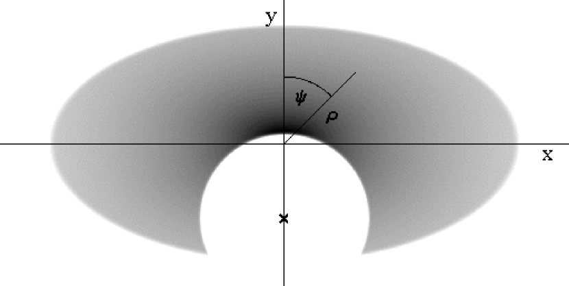
Figure 15: The surface brightness of the scattered emission in the plane of the sky (specified by $x$ and $y$ or $\rho$ and $\psi$) produced by a fully illuminated gas disk of constant mass surface density $10\,000$ years after the central source has turned off. The inclination angle of the disk is $i=60^{\mathrm{o}}$. The physical radius of the disk is 16 kpc. The center of the circle (marked by a cross) which marks the boundary between the illuminated and not illuminated parts of the disk moves with a velocity of $1.73c$ in the direction given by $\psi=\pi$. Its radius has a size of about 6 kpc and grows with time at a rate $2c$.

If a galaxy is close enough to be resolved by the Chandra X-ray telescope then it is possible to map its scattered surface brightness as a function of position on the sky. The basic formula to compute this quantity along a given line of sight is Eq. 11. In this section we are using the paraboloid approximation (see Sunyaev & Churazov 1998 or Sec. 1) to compute the integration boundaries $s_{\mathrm{min}}(t)$ and $s_{\mathrm{max}}(t)$. The paraboloid approximation is valid in this case given the large distances of extragalactic objects.

In Fig. 15 we plot the surface brightness of the scattered emission produced by a gas disk with a central, isotropic radiation source of luminosity $L_{\mathrm{agn}}=10^{44}\,{\rm erg}\,{\rm s}^{-1}$ that turned off $10\,000$ years ago. The disk has an inclination of $i=60^{\mathrm{o}}$, with $i$ defined as the angle between the line of sight and the normal direction of the disk. The figure shows that a part of the disk is not bright, because it is not illuminated anymore. The boundary of this region, which is the projection of the intersection of the paraboloid at a time $t-t_{\mathrm{o}}$ with the disk onto the plane of the sky, is a circle. As time progresses this boundary moves radially outwards from the nucleus with an apparent velocity

$$\dot{\rho}(\psi)=\frac{c\cos i}{1+\cos\psi\sin i}.$$ (24)

This velocity depends upon the position angle $\psi$, which is defined in Fig. 15. The maximum velocity of $c\cos i/(1-\sin i)$ is given for $\psi=\pi$ and the minimum velocity of $c\cos i/(1+\sin i)$ for $\psi=0$. This “motion” has the effect that the center of the circle (marked by a cross in Fig. 15) moves in the direction $\psi=\pi$ while it is growing in size. The velocity of its center is given by $v_{\mathrm{o}}=(\dot{\rho}(\pi)-\dot{\rho}(0))/2=c\,\tan i$, which is superluminal for inclination angles larger than $45^{\mathrm{o}}$. For an inclination of $i=60^{\mathrm{o}}$ this velocity is $v_{\mathrm{o}}\approx 1.73c$. The radius of the circle grows with time as $c\,t/\cos i$.

The motion of this circle and the boundary between the illuminated and not illuminated parts of the disk is an example of apparent superluminal motion produced by scattering on suitable shaped screens. This subject has been discussed in the literature by e. g. Blandford et al. (1977).

Figure 16: The scattered X-ray surface brightness as a function of projected distance from the nucleus along a fixed position angle of $\psi=\pi/2$. The solid line marks the surface brightness for the fully illuminated disk. The other lines mark the switch off (Fig. 15) and the 1000 year flare case (Fig. 19) 5000 (dot-dashed), $10\,000$ (dashed) and $20\,000$ (dotted) years after the end of the nuclear activity. The switch off case corresponds to the curves which show no brightness below a certain distance and then join on to the solution for the fully illuminated disk. The increase in surface brightness between 4 and 6 kpc is due to the molecular ring which is located at these radii. The $\rho^{-2}$ dependence described by Eq. 25 is visible.

For a face on disk ($i=0^{\mathrm{o}}$) with a constant mass surface density it is easy to see from Eq. 11 that the surface brightness drops with distance from the nucleus as $\propto\rho^{-2}$. This is still valid in the case of an inclined disk. In the limit of a uniform disk with a constant mass surface density restricted by $r=r_{\mathrm{max}}$ one can derive an analytic solution for the surface brightness of the illuminated parts of a disk with inclination $i$. It is necessary to express the factor $(1+\cos^{2}\theta_{\mathrm{sc}})/r^{2}$ appearing in Eq. 11, where $\theta_{\mathrm{sc}}$ is the scattering angle and $r$ the physical distance from the nucleus, as a function of the projected radius $\rho$, the position angle $\psi$ and the inclination angle $i$ which yields

$$I_{\nu}=\,\frac{\Sigma_{\mathrm{HI}}}{\cos i}\,\frac{L_{\mathrm{agn}}}{4\pi\rho^{2}}\,\frac{3\sigma_{\mathrm{T}}}{16\pi}\,\frac{1+2\cos^{2}\psi\tan^{2}i}{(1+\cos^{2}\psi\tan^{2}i)^{2}}.$$ (25)

As visible from Fig. 15, beyond a certain position angle the scattered surface brightness cuts off because these parts of the disk are not illuminated anymore by the central source. This angle is given by:

$$\psi_{\mathrm{max}}=\arccos\left(\frac{c^{2}t^{2}-\rho^{2}}{2\,ct\rho\tan i}\right).$$ (26)

Figure 17: The scattered X-ray surface brightness as a function of position angle at a fixed projected distance of 2 kpc from the nucleus. The different lines mark different inclination angles of the disk for the fully illuminated disk and 5000 years after switch off: $i=0^{\mathrm{o}}$ (dotted), $i=30^{\mathrm{o}}$ (dashed), $i=60^{\mathrm{o}}$ (dash-dotted) and $i=80^{\mathrm{o}}$ (solid). The switch off leads to to disappearance of the illuminated region at large position angles.

Besides this more qualitative picture we present in Figs. 16, 17 and 18 the surface brightness along several cuts of the partly illuminated disk shown in Fig. 15. These figures confirm the validity of the above formulae, Eqs. 25 and 26.

In Fig. 16 we plot the scattered surface brightness as a function of projected radius $\rho$ for a fixed position angle of $\psi=\pi/2$. The curve for the fully illuminated disk shows the $\rho^{-2}$ dependence of the surface brightness given by Eq. 25. Note that in this computation we have included a molecular ring with a two times larger mass surface density between about 4 and 6 kpc, which causes the bump between these radii. The surface brightness cuts off beyond the maximal disk radius of 16 kpc. Furthermore plotted in this figure are the surface brightness for the switch off (full picture given in Fig. 15) and the flare scenario (full picture given in Fig. 19) at different times after the end of the nuclear activity. The curves showing the surface brightness for the the flare scenario move with a velocity of about $c$ to larger projected distances as given by Eq. 24 for a position angle of $\psi=\pi/2$.

Figs. 17 and 18 show the scattered surface brightness at a fixed projected distance of $\rho=2\,{\rm kpc}$ from the nucleus as a function of position angle. For clarity no molecular ring was assumed in these two plots.

In Fig. 17 we plot the surface brightness of the scattered emission for different inclinations of the disk for the fully illuminated and the switch off case. The brightness contrast for large inclinations of the disk mainly comes about because the same projected distance at position angles $\psi=0$ and $\psi=\pi/2$ corresponds to physical distances from the nucleus differing by a factor of $(\cos i)^{-1}$. Furthermore the average scattering angle for material at a position angle of $\psi=0$ is $\theta_{\mathrm{sc}}\approx\pi/2+i$ compared to $\theta_{\mathrm{sc}}\approx\pi/2$ for a position angle of $\psi=\pi/2$. The angular dependence of the curves presented in Fig. 17 is well described by Eq. 25.

Fig. 18 shows the same quantities plotted for one disk with a large inclination of $i=80^{\mathrm{o}}$ at different times after the switch off of the central source. With increasing time the not illuminated part of the disk “works” its way towards smaller position angles. The angle where the brightness cuts off is given by Eq. 26.

Figure 18: The scattered X-ray surface brightness as a function of position angle at a fixed projected distance of 2 kpc from the nucleus. The inclination of the disk is $i=80^{\mathrm{o}}$. We plot the surface brightness for the fully illuminated disk (solid line) and 1000, 3000, $10\,000$, $30\,000$ and $50\,000$ years (dotted lines from right to left) after the switch off of the central radiation source.

In Fig. 19 we show how structure in the same disk as in the previous figures is probed by a flare of the nucleus. This case might be relevant for spiral galaxies like Andromeda, where the neutral gas is very concentrated in a ring. We map the surface brightness of the scattered emission produced by a gas disk with a 2 kpc broad molecular ring at 5 kpc, with a mass surface density two times larger than the other parts of the disk, illuminated by a flare of the central source of $1000$ years duration at different times after the end of the flare. The velocity of the light front behind (or above) the nucleus is much smaller than the superluminal one in front (or below) of the source. As time progresses the light front scans along the molecular ring. GMCs will lighten up and and produce flares in the response. With the spatial resolution of Chandra one should be able to resolve these clouds in a galaxy up to a distance of about 10 Mpc. The characteristic time of these events is rather short.

At a certain point the lower, faster light front reaches the edge of the gas disk. The “ring” will start to break up and a luminous arc travels upwards, slowly fading away as it reaches larger distances.

Obviously a flare due to the tidal disruption of a star in the nucleus with a duration of the order of a few years will produce a feature in the scattered surface brightness distribution of smaller width than the one shown in Fig. 19. If the tidal disruption rate is large enough, of the order of $10^{-4}\,{\rm year}^{-1}$, one might find several of these arcs per galaxy.

5.2 Scattered X-ray luminosity

For a source too distant to be resolved by X-ray telescopes the measurable quantity is the scattered flux from which one can derive a scattered luminosity. In this section we compute the scattered luminosity of a spiral galaxy with the same neutral gas distribution as our Galaxy in response to the above assumed forms of activity of its nucleus.

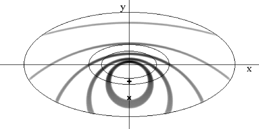
Figure 19: The surface brightness of the scattered emission produced by a gas disk with a 2 kpc broad molecular ring at 5 kpc illuminated by a flare of the central source of $1000$ years duration having occured $5000$, $10\,000$, $20\,000$, $40\,000$ and $60\,000$ years ago. The edges of the gas disk at 16 kpc and the the molecular ring at 4 and 6 kpc are marked by solid ellipses. The inclination angle of the disk is $i=60^{\mathrm{o}}$. The centers of the “rings” $5000$ and $10\,000$ year after the end of the flare have been marked by a plus sign and a cross. Note how with progressing time the flare scans along the molecular ring. The highest surface brightness regions, besides the one close to the nucleus, are where the flare intersects with the molecular ring.

Fig. 20 shows the scattered luminosity after the AGN has switched off as a function of time for different inclinations of the disk. As parameters we choose as before $L_{\mathrm{agn}}=10^{44}\,{\rm erg\,s}^{-1}$ and a constant HI distribution $\Sigma_{\mathrm{HI}}=4\,M_{\odot}\,{\rm pc}^{-2}$ up to 16 kpc.

The different luminosities for different inclinations at times $t-t_{\mathrm{o}}\leq 0$, when the whole disk is illuminated, come about because of the angular dependence of the differential scattering cross-section. For a face on disk $i=0^{\mathrm{o}}$ the scattering angle is obviously $\pi/2$. Because the differential cross-section for Thomson scattering is minimal for an angle of $\pi/2$ the face on disk has the smallest scattered luminosity. The much stronger differences at larger times are due to the superluminal motion of the light front. It leads to the strong effects in the low luminosity tail. Note the similarity of these curves with the ones of the scattered flux produced by the Galactic HI distribution in response to a switch off or a flare of Sgr A^∗ (Figs. 11 and 12). The edge on case ($i=90^{\mathrm{o}}$) is similar to the case of the observer located inside the Milky Way looking at small Galactic longitudes. The X-ray binary population of the Milky Way produces a luminosity of about $2\times 10^{39}\,{\rm erg}\,{\rm s}^{-1}$ in the 2-10 keV range (Grimm et al. 2001). It will be therefore difficult to detect the scattered signal below this limit.

Figure 20: The scattered X-ray luminosity observable at a time t produced by a spiral galaxy with the HI distribution of the Milky Way in response to its central radiation source switching off at a time $t_{\mathrm{o}}$. The assumed luminosity of the AGN is $10^{44}\,{\rm erg}\,{\rm s}^{-1}$. The different curves are for an inclination angle of the disk of $90^{\mathrm{o}}$ (solid), $60^{\mathrm{o}}$(dot-dashed), $30^{\mathrm{o}}$ (long dashed) and $0^{\mathrm{o}}$ (dashed). The dotted line marks the Galactic luminosity produced by X-ray binaries.

For the face on disk ($i=0^{\mathrm{o}}$) one can derive a simple analytic solution for the scattered luminosity as a function of time. In this case the illuminated and not illuminated parts are concentric disks (switch off or switch on scenario) or annuli (flare scenario). The problem therefore is axially symmetric and the projected distance $\rho$ is equivalent to the physical distance $r$ from the nucleus. Imagine the disk to made up of small mass elements ${\rm d}M=\Sigma(\rho)\,{\rm d}A=\Sigma(\rho)2\pi\rho{\rm d}\rho$. If the mass element is illuminated it contributes a fraction ${\rm d}L\propto{\rm d}M/\rho^{2}$ (Eq. 14) to the scattered luminosity. The total scattered luminosity at a time $t$ is just the integral over all the illuminated mass elements

$$L_{\mathrm{sc}}(t)=\int{\rm d}L\propto\int_{a(t)}^{b(t)}\frac{\Sigma(\rho)\,{\rm d}\rho}{\rho}.$$ (27)

For a constant mass surface density $\Sigma(\rho)=\Sigma_{\mathrm{HI}}$ one obtains the simple solution

$$L_{\mathrm{sc}}(t)=L^{\mathrm{sc}}_{\mathrm{o}}\ln\frac{b(t)}{a(t)},$$ (28)

with

$$L^{\mathrm{sc}}_{\mathrm{o}}=2\times 10^{39}\,{\rm erg\,s}^{-1}\,\left(\frac{L_{\mathrm{agn}}}{10^{44}\,{\rm erg\,s}^{-1}}\right)\left(\frac{\Sigma_{\mathrm{HI}}}{4\,M_{\odot}\,{\rm pc}^{-2}}\right).$$

For the face on disk the ellipsoids travel with the velocity of light radially outward and the the inner and outer radius for the flare scenario can be be described as $a(t)=ct$ and $b(t)=c(t+\Delta)$. For the switch off scenario one has $b(t)=\rho_{\mathrm{max}}$ and for the switch on case $a(t)=0$. This simple analytic formula helps to understand the behaviour of the curves presented in Fig. 21, which are the results of our numerical integration. For large times the flare solutions join with the switch off solution. This happens when only the outer parts of the disk of size corresponding to the flare duration are still scattering.

Figure 21: The scattered X-ray luminosity observable at a time t produced by a face on disk ($i=0^{\mathrm{o}}$) with the HI distribution of the Milky Way in response to flares of the central radiation source of different durations ending at a time $t_{\mathrm{o}}$: $1000$ years (dashed), $3000$ years (long dashed) and $10\,000$ years (dot-dashed). The solid line shows the switch off case. The assumed luminosity of the AGN is $10^{44}\,{\rm erg}\,{\rm s}^{-1}$. The dotted line marks the Galactic luminosity produced by X-ray binaries.

5.3 Fluorescent iron K_α-line luminosity

Scattering of X-rays produced by a powerful AGN is accompanied by X-ray photo absorption by heavy elements and emission in the narrow fluorescent K_α-lines. The iron K_α-line at 6.4 keV is the brightest spectral emission feature in the scattered radiation. Its equivalent width in the scattered X-ray flux is close to 1 keV for a normal cosmic abundance of iron (Vainshtein & Sunyaev 1980). The time dependence of the K_α-line luminosity should repeat that of the scattered continuum. The main difference is that scattering in the K_α-line is isotropic. The results for the K_α-line fluorescence line should therefore differ by a factor of two or less and follow similar trends as presented in the previous figures. For example if we would plot the luminosity in the K_α-line in Fig. 20 the differences for times before the switch off would disappear and one would get the same luminosity for all disks independent of inclination. Since the narrow K_α-line originating in Galactic X-ray binaries has a very low equivalent width, observations of the fluorescent, iron K_α-line are a more promising way to detect the scattered radiation produced by a faded flare of Sgr A^∗.

6 Discussion

In this paper we have presented upper limits on the hard X-ray luminosity of Sgr A^∗ in the recent past. As the scattering material we have considered molecular and neutral atomic hydrogen present in the Galactic Disk. The CO and X-ray data we had access to, have allowed us to derive limits for the 4-10 keV luminosity of Sgr A^∗ down to about $8\times 10^{40}\,{\rm erg\,s}^{-1}$ at certain times. For other times the limits are of the order of $10^{41}-10^{42}\,{\rm erg\,s}^{-1}$. Now we want to briefly address a few points which demand some further discussion:

• In simulating the activity of the GC we made the assumption that the emission of Sgr A^∗ was isotropic. Studies of AGN show that their radiation field is often anisotropic due to the presence of a relativistic jet or as a result of shielding by a molecular torus. A jet produced by Sgr A^∗ would probably point away from the Galactic plane. This would make our derived limits weaker.

• Ebisawa et al. (2001) have reported the results of a deep Chandra observation of a Galactic plane region ($l=28.45^{\mathrm{o}},b=-0.2^{\mathrm{o}}$), which is devoid of known X-ray point sources. The total X-ray flux in the 2-10 keV range is determined to be $\sim 1.1\times 10^{-10}\,{\rm erg}\,{\rm s}^{-1}{\rm deg}^{-2}$. About ten per cent of this flux is accounted for by point sources resolved by Chandra. These are extragalactic sources seen through the Galactic disk. 90 % of the observed flux is due to diffuse emission at the level of the sensitivity and the angular resolution of Chandra. This diffuse flux is within a factor of two of the ones measured by ASCA in nearby fields, which are of the order of $\sim 6\times 10^{-11}\,{\rm erg}\,{\rm s}^{-1}{\rm deg}^{-2}$ (Sugizaki et al. 2001). Unfortunately none of the GMCs listed in the SRBY87 sample lies in this field, but the HI column density in this direction is about $2\times 10^{22}\,{\rm cm}^{-2}$, similar to the one in the ASCA fields. Improvements might result from the spectral data obtained by XMM-Newton. If XMM-Newton will be able to detect the K_α-line of neutral iron in the same field this will open the possibility to separate the scattering contribution.

• The Trapezium region ($l=209.01^{\mathrm{o}},b=-19.38^{\mathrm{o}}$) of the Orion Nebula has recently been observed by Chandra (Schulz et al. 2001). An upper limit for the diffuse emission in the energy range 0.1-10 keV of $2\times 10^{28}\,{\rm erg}\,{\rm s}^{-1}{\rm arc\,sec}^{-2}$ is derived, which corresponds to a diffuse flux of $\sim 1\times 10^{-8}\,{\rm erg}\,{\rm s}^{-1}{\rm deg}^{-2}$. The distance towards the Orion nebula is $\approx 440$ pc, corresponding to a time delay of $\sim 2400$ years. The galactocentric distance of Orion is $R\sim 8.8$ kpc. The measured H₂ column density in this direction is $3.2\times 10^{22}\,{\rm cm}^{-2}$, which translates into an upper limit for the luminosity of Sgr A^∗ of $3\times 10^{41}\,{\rm erg}{\rm s}^{-1}$. So GMCs in our vicinity might give comparable limits to the ones derivable from GMCs located in the molecular ring, but their time delays will be only of the order of their distances.

An obvious next step would be to apply this method to constrain the luminosity of Sgr A^∗ in the past to GMCs and HI gas with still larger distances from the GC and thereby extending our time coverage. Because the scattered luminosity is proportional to $M_{\mathrm{gas}}/R^{2}$, there certainly will be a limit up to what distances we will obtain meaningful results with this method.

A reservoir of neutral gas which has the potential to scatter the radiation emitted by Sgr A^∗ at even larger distances and therefore longer time delays is the LMC. With a distance of $\sim 50$ kpc from the sun the time delay turns out to be $\sim 250\,000$ years. Unfortunately the existing data does not permit to obtain interesting limits upon the X-ray luminosity of Sgr A^∗. We therefore should wait for XMM-Newton observations of the iron K_α-line in the direction towards massive gas complexes in the LMC.

- (1) Alcock, C., & Hatchett, S. 1978, ApJ, 222, 456
- (2) Baganoff, F. K., Maeda, Y., Morris, M., Bautz, M. W., Brandt, W. N., Cui, W., Doty, J. P., Feigelson, E. D., Garmire, G. P., Pravdo, S. H., Ricker, G. R., & Townsley, L. K. 2001, astro-ph/0102151, ApJ in press
- (3) Blandford, R. D., McKee, C. F., & Rees, M. J. 1977, Nature, 267, 211
- (4) Binney, J., & Merrifield, M. 1998, “Galactic Astronomy”, Princeton University Press, Princeton
- (5) Blitz, L., & Williams, J. P. 1999, in “The Origin of Stars and Planetary Systems”, eds. Lada, C. J., Kylafis, N. D., p. 3
- (6) Couderc, P. 1939, Ann. d’Astrophys., 2, 271
- (7) Dame, T. M. 1993, in “Back to the Galaxy”, AIP Conference Proceedings 278, eds. Holt, S. S., Verter, F., p. 267
- (8) Dame, T. M., Hartmann, D., & Thaddeus, P. 2001, ApJ, 547, 792
- (9) Dickey, J. M., & Lockman F. J. 1999, ARAA, 28, 215
- (10) Ebisawa, K., Maeda, Y., Kaneda, H., & Yamauchi, S. 2001, Sciencexpress, 10.1126/science.1063529
- (11) Garcia, M. R., Murray, S. S., Primini, F. A., Forman, W. R., McClintock, J. E., & Jones, C. 2000, ApJ, 537, 23
- (12) Genzel, R., Eckart, A., Ott, T., & Eisenhauer, F. 1997, MNRAS, 291, 219
- (13) Ghez, A. M., Klein, B. L., Morris, M., & Becklin, E. E. 1998, ApJ, 509, 678
- (14) Gilfanov, M. R., Sunyaev, R. A., & Churazov, E. M. 1987, SvAL, 13, 233
- (15) Grimm, H.-J., Gilfanov, M. R., & Sunyaev, R. A. 2001, forthcoming paper
- (16) Kaaret, P. 2001, astro-ph/0106568, ApJ in press
- (17) Koyama, K., Makishima, K., & Tanaka, Y. 1986, PASJ, 38, 121
- (18) Koyama, K., Maeda, Y., Sonobe, T., Takeshima, T., Tanaka, Y., & Yamauchi, S. 1996, PASJ, 48, 249
- (19) Kormendy, J., & Gebhardt, K. 2001, astro-ph/0105230, to appear in “The 20th Texas Symposium on Relativistic Astrophysics”, eds. Martel, H., & Wheeler, J. C., AIP, in press
- (20) Lee, Y., Stark, A. A., Kim, H. G., & Moon, D. 2001, astro-ph/0101004, ApJ in press
- (21) Madau, P., Blandford, R. D., & Rees, M. J. 2000, ApJ, 541, 712
- (22) McKee, C. F., & Ostriker, J. P. 1977, ApJ, 218, 148
- (23) Morrison, P., & Sartori, L. 1969, ApJ, 158, 541
- (24) Morrison, R., & McCammon, D. 1983, ApJ, 270, 119
- (25) Murakami, H., Koyama, K., Sakano, M., Tsujimoto, M., & Maeda, Y. 2000, ApJ, 534, 283
- (26) Murakami, H., Koyama, K., Tsujimoto, M., Maeda, Y., & Sakano, M. 2001A, ApJ, 550, 297
- (27) Murakami, H., Koyama, K., & Maeda, Y. 2001B, astro-ph/0105273, ApJ in press
- (28) Nieten, C. 2001, PhD Thesis, University of Bonn
- (29) Pence, W. D., Snowden, S. L., Mukai, K., & Kuntz, K. D. 2001, astro-ph/0107133, ApJ in press
- (30) Peterson, B. M. 1993, PASP, 105, 247
- (31) Rees, M. J. 1988, Nature, 333, 523
- (32) Schulz, N. S., Canizares, C., Huenemoerder, D., Kastner, J. H., Taylor, S. C., & Bergstrom, E. J. 2001, ApJ, 549, 441
- (33) Shirey, R., Soria, R., Borozdin, K., Osborne, J. P., Tiengo, A., Guainazzi, M., Hayter, C., La Palombara, N., Mason, K., Molendi, S., Paerels, F., Pietsch, W., Priedhorsky, W., Read, A. M., Watson, M. G., & West, R. G. 2001, A&A, 365, 195
- (34) Shakura, N. I., & Sunyaev, R. A. 1973, A&A, 24, 337
- (35) Skibo, J. G., Johnson, W. N., Kurfess, J. D., Kinzer, R. L., Jung, G., Grove, J. E., Purcell, W. R., Ulmer, M. P., Gehrels, N., & Tueller, J. 1997, ApJ, 483, 95
- (36) Sofue, Y., & Kato, T. 1981, PASJ, 33, 449
- (37) Solomon, P. M., Rivolo, A. R., Barrett, J., & Yahil, A. 1987, ApJ, 319, 730 (SRBY87)
- (38) Solomon, P. M., & Rivolo, A. R. 1989, ApJ, 339, 919
- (39) Sugizaki, M., Mitsuda, K., Kaneda, H., Matsuzaki, K., Yamauchi, S., & Koyama, K. 2001, ApJS, 134, 77
- (40) Sunyaev, R. A. 1982, SvAL, 8, 175
- (41) Sunyaev, R. A., Markevitch, M., & Pavlinsky, M. 1993, ApJ, 407, 606
- (42) Sunyaev, R. A., & Churazov, E. M. 1996, Astro. Lett., 22, 648
- (43) Sunyaev, R. A., & Churazov, E. M. 1998, MNRAS, 297, 1279
- (44) Sunyaev, R. A., Gilfanov, M., & Churazov, E. M. 1998, in “Highlights in X-ray Astronomy”, eds. Aschenbach, B., Freyberg, M., p. 102
- (45) Sunyaev, R. A., Uskov, D. B., & Churazov, E. M. 1999, Astro. Lett., 25, 199
- (46) Vainshtein, L. A., & Sunyaev, R. A. 1980, SvAL, 6, 353
- (47) Valinia, A., & Marshall, F. E. 1998, ApJ, 505, 134
- (48) Williams, J. P., Blitz, L., & Stark, A. A. 1995, ApJ, 451, 252
- (49) Yang, Y., Wilson, A. S., & Ferruit, P. 2001, astro-ph/0108166, ApJ in press
- (50) Young, A. J., Wilson, A. S., & Shopbell, P. L. 2001, ApJ, 556, 6