Cluster Galaxy Evolution from a New Sample of Galaxy Clusters at 0.3 $<z<$ 0.9

Abstract

We analyze photometry and spectroscopy of a sample of 63 clusters at 0.3 $\leq z\leq$ 0.9 drawn from the Las Campanas Distant Cluster Survey to empirically constrain models of cluster galaxy evolution. Specifically, 1) by combining $I-$band photometry of 44 of our clusters with that of 19 clusters from the literature (Aragon-Salamanca et al. ; Smail et al. ; Stanford et al. ) we parameterize the redshift dependence of $M^{*}_{I}$ in the observed frame as $M^{*}_{I}=(-21.74\pm 0.12)-(0.88\pm 0.24)z-5\log h$ (rms deviation = 0.34) for $0.3\leq z\leq 0.9$ ($\Omega_{0}=0.2$, $\Omega_{\Lambda}=0$)); 2) by combining 30 of our clusters and 14 clusters from the literature (Aragon-Salamanca et al. ; Smail et al. ; Stanford et al. ) with $V$ and $I$ data we parameterize the redshift dependence of the $V-I$ color of the E/S0 red sequence in the observed frames as $V-I=(-0.24\pm 0.28)+(7.42\pm 1.03)z-(4.61\pm 0.91)z^{2}$ (rms deviation = 0.16) for $0.3\leq z\leq 0.9$; and 3) by combining 13 of our clusters with 15 clusters from the literature (Aragon-Salamanca et al. ; Stanford et al. ) with $I$ and $K^{\prime}$ data we parameterize the redshift dependence of the $I-$$K^{\prime}$ color of the E/S0 red sequence in the observed frames as $I-$$K^{\prime}$ $=(0.66\pm 0.65)+(9.50\pm 3.72)z-(14.72\pm 7.01)z^{2}+(8.72\pm 4.29)z^{3}$ (rms deviation = 0.18) for $0.3\leq z\leq 0.9$. Using the peak surface brightness of the cluster detection, $\Sigma$, as a proxy for cluster mass (Gonzalez et al. ), we find no correlation between $\Sigma$ and M${}^{*}_{I}$ or the location of the red envelope in $V-I$. We suggest that these observations can be explained with a model in which luminous early type galaxies (or more precisely, the progenitors of current day luminous early type galaxies) form the bulk of their stellar populations at high redshifts ($\gtrsim 5$) and in which many of these galaxies, if not all, accrete mass either in the form of evolved stellar populations or gas that causes only a short term episode of star formation at lower redshifts ($1.5<z<2)$. Our data are too crude to reach conclusions regarding the evolutionary state of any particular cluster or to investigate whether the morphological evolution of galaxies matches the simple scenario we discuss, but the statistical nature of this study suggests that the observed evolutionary trends are universal in massive clusters.

1. Introduction

High redshift clusters provide an excellent laboratory with which to study the evolution of galaxies in dense environments. By investing a modest amount of telescope time obtaining spectra of a handful of galaxies, thereby verifying the reality of the cluster and ascertaining its redshift, one is rewarded with the knowledge of distances to tens or even hundreds of galaxies. The spectral and photometric properties of these galaxies can then be used to constrain evolutionary models, whose differences usually become appreciable at high redshift, $z>0.5$ (cf. Bruzual & Charlot 1993; Kauffmann et al. 1998). Until recently, such efforts have been hampered by the small number of known high redshift clusters. Published work in this field relies upon the examination of the same $\sim$dozen clusters, drawn primarily from two optical surveys. Both of these surveys (Gunn, Hoessel, & Oke 1986, hereafter GHO; Couch et al. 1991, hereafter C91) selected objects on the basis of an overdensity of resolved objects. GHO’s efforts yielded 8 clusters with $z\geq 0.55$, while C91 yielded 3.

Because the number of known high redshift clusters is small, they have been studied in great detail by many authors. In particular, with the advent of the Keck telescopes and the Hubble Space Telescope (HST), detailed information regarding the cluster galaxies’ star formation rates and morphologies have complemented the more traditional ultraviolet, optical, and infrared photometry. As a result, a comprehensive picture of the formation and evolution of cluster galaxies has begun to emerge in which many, if not all, galaxies have experienced some recent star formation. The most active class of galaxies was first noted by Butcher & Oemler (1984, B-O). They studied 33 clusters of galaxies with 0.003$\leq z\leq$0.54 and discovered that the fraction of blue galaxies increased markedly with redshift. They interpret the rise in blue fraction as evidence for increased star formation in the past and this interpretation has subsequently been confirmed by spectroscopic studies (Dressler & Gunn 1982, 1983, 1992; Couch & Sharples 1987; Couch et al. 1994; Abraham et al. 1996; Fisher et al. 1998; Poggianti et al. 1999). Furthermore, morphological classifications using high resolution HST imaging show that the bulk of these star-bursting galaxies are disk dominated systems, a significant fraction of which show signs of interactions or mergers (Couch et al. 1994, 1998; Dressler et al. 1994, 1999; Oemler, Dressler, & Butcher 1997; Poggianti et al. 1999).

Cohabitating with these active galaxies, however, is a seemingly quiescent population. These galaxies are the cluster’s brightest and reddest, which lie along a very narrow locus in the cluster color-magnitude (CM) diagram referred to as the red envelope. Detailed morphological and spectroscopic studies of clusters at high redshift confirm that these galaxies are a subset of the cluster’s elliptical population (e.g. de Propris et al. 1999; van Dokkum et al. 1999). Evolution of the zeropoint, slope, and scatter about cluster CM relations all suggest that these ellipticals formed at a very high redshift ($z\gtrsim 5$) and have experienced little or no recent star formation (see Aragon-Salamanca et al. 1993, hereafter A93; Rakos & Schombert 1995, hereafter RS; Ellis et al. 1997; Stanford et al. 1998, hereafter SED98; Jones et al. 2000), while work on the evolution of the fundamental plane (Kelson et al. 2000) and on the evolution of absorption line indicies (Bender, Ziegler, & Bruzual 1996; Kelson et al. 2001) support this conclusion by placing a lower redshift limit of $\sim 2.5$ for the formation of the bulk of the stellar populations. Studies of the optical and infrared luminosity functions of cluster galaxies suggest a more moderate formation redshift for cluster ellipticals, $z\gtrsim 2$ (Smail et al. 1997, hereafter S97; de Propris et al. 1999). Despite this general consensus, the non-uniqueness of spectral synthesis models, against which the majority of these observations are compared, allows for the possibility that at least some of these galaxies are not completely quiescent. In fact, recent work by van Dokkum et al. (1999) suggests that a large fraction of these galaxies in the higher redshift ($\sim 1$) clusters are not relaxed systems. These authors studied MS1054-03 at $z=0.83$ using spectroscopy and HST high resolution imaging and found that 17% of the L$>$L_∗ cluster population is experiencing a major merger, most of which will probably evolve into luminous (2L_∗) elliptical galaxies. They estimate that $\sim$50% of the present-day cluster ellipticals were assembled in mergers since $z\sim 1$, assuming that the galaxy population of MS1054-03 is representative. While most of the mergers involve red early-type galaxies with no detected [OII] $\lambda$3727 emission, some do exhibit enhanced Balmer absorption indicative of a modest recent starburst. Consequently, the question of the evolutionary history of the brightest cluster ellipticals remains open.

As mentioned previously, all of the above work is hampered by the lack of statistically significant samples. General conclusions based on small samples rely critically on the assumption that this handful of clusters is representative of the entire high redshift cluster population. This assumption is particularly worrisome when (1) it is viewed in the context of a hierarchical clustering scenario which holds that structures of different mass scales form at different times and consequently have experienced different evolutionary histories, and (2) one realizes that the cluster properties play a significant role in their original identification. The need for a large, well-defined, high redshift cluster sample is evident.

In an attempt to resolve issues raised by small sample size, Postman et al. (1996) conducted the Palomar Distant Cluster Survey. This survey consists of optical/near IR imaging of a $\sim$5 deg² area using the 4-shooter CCD camera on the Palomar 5m telescope. Their cluster finding technique was more sophisticated than previous optical surveys by incorporating magnitude and color filters to minimize the contamination from line-of-sight projections. Their method relies upon resolving distant galaxies in two colors and thus requires the use of a large telescope under photometric conditions with good seeing, which limits the areal coverage of the survey. Their efforts yielded a large, well-defined cluster catalog that contains 35 clusters with estimated redshifts $\geq$0.5, plus 25 clusters from an inhomogeneous sample with estimated redshifts $\geq$0.5 (the PDCS includes clusters identified previously by GHO). Using these clusters to study galaxy evolution, their results to date provide more statistically significant confirmation of the trends observed with smaller samples. In particular, Lubin (1996) examined the location of the red envelope in the HST filters $V_{4}-I_{4}$ ($V_{4}$ = F555W and $I_{4}$ = F785LP) and found that the data are most consistent with the passive evolution of an elliptical galaxy that formed at high redshift. She also measured the fraction of blue galaxies, f_b, and found an increase in f_b with redshift, consistent with a high redshift extension of the Butcher-Oemler effect.

An alternative, efficient method for finding high redshift clusters was developed by Dalcanton (1996). This technique capitalizes on the idea that the total flux from a distant cluster in shallow images is dominated by the flux from unresolved sources. If one has an intrinsically uniform image, the flux from the unresolved sources produces a detectable low surface brightness fluctuation. Because the technique does not rely upon an overdensity of resolved objects, relatively shallow (but highly uniform) exposures are sufficient to identify distant clusters and a much larger area on the sky can be surveyed. Dalcanton et al. (1997) verified the ability of this technique to detect LSB objects to the required central surface brightness using existing scans from a $\sim 17.5$ deg² Palomar 5m survey (originally taken as part of the Palomar Transit Grism Survey for high redshift quasars; Schneider et al. 1994). This survey identified more than 50 northern hemisphere cluster candidates. In 1995, the authors conducted a 130 deg² drift-scan survey of the southern sky at the Las Campanas Observatory. The reductions and object identification is complete and the final cluster catalog contains over 1000 cluster candidates (Gonzalez et al. 2001). Not only does this catalog result in a tremendous increase in the number of known clusters at these redshifts, but because our cluster identification criteria is independent of those utilized in previous surveys, this catalog provides an independent, well-defined sample with which to compare the results of more traditional surveys.

In this paper, we present the first study of galaxy evolution using a subset of the Las Campanas Distant Cluster Survey. In addition to 54 southern clusters, we include 9 northern clusters drawn from the Palomar survey. The combined sample consists of 63 clusters, 17 of which are spectroscopically confirmed and 46 of which have photometrically estimated redshifts. We obtain deep follow-up imaging in $V$, $I$, and $K^{\prime}$ , although not every cluster is imaged in every band. We use these data, along with that of 19 clusters from the literature, to classify cluster candidates, photometrically estimate their redshifts, and study the luminosity and color evolution of cluster galaxies. In §2 we briefly describe the survey, including cluster candidate identification, and our follow-up observations. In §3 we present our three photometric redshift estimation techniques. In §4 we utilize our clusters with spectroscopic redshifts and those with photometric redshifts to trace the evolution of cluster galaxies in luminosity and color. Specifically, we examine the evolution of M${}^{*}_{I}$ and the location of the red envelope in $V-I$ and $I-$$K^{\prime}$ . We investigate cluster selection biases and their effect on our empirically measured galaxy evolution in §4.4. In §4.5 we combine our results with those from the recent literature and suggest a picture of cluster galaxy formation and evolution. Finally, we summarize our results and conclusions in §6.

2. The Data

Our data originate from a variety of telescopes and instruments. The candidate galaxy clusters are identified using drift scan images and techniques described briefly below for context, but in full detail by Gonzalez et al. 2001. We then describe the follow-up spectroscopy and photometry of subsamples of candidate galaxy clusters that constitute the core dataset for this study.

2.1. Cluster Identification

Our candidate clusters are drawn from two optical drift scan surveys. The first is a $\sim 17.5$ deg² Palomar 5m survey using the 4-shooter camera (Gunn et al. 1987) and the F555W “wide $V$” filter described by Dalcanton et al. (1997). Dalcanton et al. made use of existing scans (originally taken as part of the Palomar Transit Grism Survey for high redshift quasars; Schneider et al. 1994) to verify the low surface brightness (LSB) technique for detecting LSB objects to the required central surface brightness first proposed in detail by Dalcanton (1996). This survey identified more than 50 northern hemisphere cluster candidates. The second is a 130 deg² survey of the southern sky conducted at the Las Campanas Observatory 1m telescope over 10 nights by the authors using the Great Circle Camera (Zaritsky, Shectman, & Bredthauer 1996) and a wide filter, denoted as $W$, that covers wavelengths from 4500 Å to 7500 Å. This survey was specifically designed to study LSB galaxies and high redshift galaxy clusters. Scans are staggered in declination by half of the field-of-view (24 arcmin) so that each section of the survey is observed twice, but with a different region of the detector. Exposure times are limited by the sidereal rate, which at the declination of the survey ($-10^{\circ}$ to $-12^{\circ}$) is $\sim$97 sec. The pixel scale is 0.7 arcsec/pixel with a typical seeing of about 1.5 arcsec. The full region surveyed measures $\sim 85^{\circ}\times 1.5^{\circ}$ and is embedded within the area covered by the LCRS (Shectman et al. 1996). The result of iterative flatfielding, masking, filtering, and object detection is a catalog of $\sim$ 1000 cluster candidates (a full description of the method and catalog are provided by Gonzalez et al. 2001).

The focus of this study is the photometry and spectroscopy of subsamples of candidate clusters obtained to test cluster identification algorithms and study the clusters’ galaxy populations. Keck spectroscopy, optical ($V$- and $I$-band) photometry, and IR ($K^{\prime}$-band) photometry are presented, although not all types of data are available for every candidate. Table 1 contains information only about those candidates that we determine to be bonafide clusters, rather than all observed candidates. The name of the cluster is listed in the first column. RA and DEC (2000.0) are in the next column, where the center of the cluster is taken to coincide with the centroid of the low surface brightness fluctuation. The last six columns contain the exposure time and seeing for each of the three photometric bands, $V$, $I$, and $K^{\prime}$ . In summary, 97$\%$ of our clusters are imaged in $I$, $54\%$ in $V$, $33\%$ in $K^{\prime}$ , and $29\%$ have spectroscopy. Some clusters were imaged twice in various photometric bands. Because objects were observed on different runs (sometimes with a different camera and/or telescope) and calibrated using different sets of standard stars, they often have two completely independent sets of photometry. We use both sets independently in the calibration of our photometric redshift estimators and subsequent analysis.

These data provide a set of confirmed clusters with which to develop a set of quantitative statistical descriptors to use for cluster selection and a statistical sample of clusters with which to study galaxy evolution in clusters. Because we were testing our cluster selection algorithms, the cluster subsample is heterogeneous. It includes both some of our best and some of our worst candidates. Because our selection criteria evolved during this study, some of the confirmed candidates presented here will not be in our final cluster catalog. No biases in galaxy properties, except those that possibly correlate with cluster properties such as concentration and richness (parameters that factor into the cluster selection), are expected. This issue will be discussed in more detail in §4.

2.2. Spectroscopy

Two critical cluster parameters for any subsequent study of our catalog are the cluster redshifts and the masses (or alternatively to mass, richness, X-ray luminosity, or velocity dispersion, albeit with different caveats). With a catalog of $\sim$ 1000 cluster candidates, it is not feasible to obtain spectroscopy or deep follow-up photometry for every candidate. Consequently, it is imperative to develop efficient observational estimators of these parameters. We present and evaluate several redshift estimators.

In December 1995, we began an observing program that combines long-slit spectroscopy obtained using the Keck telescopes and optical and infrared photometry obtained using the Las Campanas 2.5m and 1m telescopes, the Palomar 1.5m, and the Lick 3m. Our basic goal is to identify and calibrate photometric redshift estimators. These data have two additional functions: 1) they enable us to confirm candidate clusters and tune our selection criteria, and 2) they enable us to study the clusters themselves and their galaxy populations.

Spectra were obtained using the Low-Resolution Imaging Spectrograph (Oke et al. 1995) on the Keck I telescope on 1995 December 20-21, 1997 March 14-15, 1998 April 4-5, and 1999 March 20-21. Due to weather and technical problems $\sim$ 40% of the time was usable. The deep imaging necessary to construct multi-object masks was generally not available so we used a single long slit with a 600 line mm^-1 grating. The slit was aligned, using the guider image, to include as many individual galaxies as possible (generally 2 to 3 with m${}_{R}\lesssim 22$) and to lie across the position of the LSB feature detected in the scans. As an interesting aside, the Keck guider images are deeper than the drift scan images from which the candidates are selected. Typical spectroscopic exposure times were 30 minutes to one hour. Preliminary results from this work are discussed by Zaritsky et al. (1997).

The reduction of these spectra is standard. Images are rectified and calibrated using calibration-lamp exposures and night sky lines (see Kelson et al. 1997 for details). Velocities are measured using a cross-correlation technique or by measuring centroids of emission lines. The rms redshift difference between redshifts measured from different emission lines in the same spectra is 0.0033 (typically less than 0.0005). In cases where only one emission line is observed, we attribute it to H$\beta$. Little ambiguity exists between H$\beta$ and [OII] because the [OII] emission line is a resolved doublet (3726 and 3729 Å).

The distribution of galaxy redshifts is shown in Figure 1 for all 28 fields observed. We consider a candidate object to be a real cluster if at least three galaxies cluster within 1000 km s^-1 of their mean redshift. A valid concern is that “successful” candidates in this scheme may arise randomly in lines-of-sight through large-scale structures. If random large scale structures appeared in 19 of 28 fields (60%), then we would expect to find two coherent structures in 13 of our fields. Only one such field exists, and so it is evident that random redshift associations are not the dominant cause of the redshift associations. However, to test whether random redshift associations are significant, we use published Keck LRIS spectroscopy (Guzman et al. 1997; Lowenthal et al. , 1997; Phillips et al. 1997; Vogt et al. 1997; Cohen et al. 2000) out to $z=1.1$ to estimate the likelihood of chance redshift associations. The use of data from the same instrument as used in this study ensures that the data are of comparable quality and have similar systematic problems (sky lines, fringing) over the same redshift range. The joint catalog contains coordinate positions and redshifts for 686 galaxies at $0.3<z<1.1$ (a redshift range chosen to match that of our sample). We then randomly select fields with the same distribution of galaxies per field as seen in Figure 1. The number of pairs of galaxies within 1000 km sec^-1 predicted for our sample from 10,000 simulations is 9.9 (we observe 7, which is within the 1$\sigma$ Poisson fluctuation). The number of triplets predicted is 1.3 (consistent with the one system in which two structures are seen, although this is not necessarily the spurious system). Only four of our successful 19 cluster candidate have the minimum three members. The number of quadruples predicted in this sample is 0.2 (we observe 15). We conclude that systems with three or more galaxies within 1000 km sec^-1 are overwhelmingly not the result of random lines of sight through large-scale structures. This conclusion will later be confirmed by the independent correspondence of the magnitude of the brightest galaxy in each cluster candidate, the mean spectroscopic redshift of the galaxies in the overdensity, and the concentration of galaxies at the position of the original LSB detection. We conclude that our success rate for identifying true clusters is $\gtrsim$ 60%, and that perhaps it is substantially greater. This success rate will be confirmed independently by other means below.

2.3. Optical Photometry

$V$- and $I$-band images, which straddle the Ca II H & K break for galaxies at redshifts of $0.3\lesssim z\lesssim 0.9$, provide a measure of the stellar populations in these galaxies. Because the majority of our photometry was completed before the cluster finding algorithm was fine-tuned (indeed it was necessary to help train the algorithm), we imaged some candidates only in $I$, to provide more images of potential clusters at the expense of color information. Optical photometry in the Johnson $V$-band and Cousins $I$-band for the northern hemisphere clusters was obtained at the Palomar 1.5 m telescope during 1996 May 9-14. Conditions during this run were rather poor due to intermittent cirrus with seeing ranging from 2^′′ to 3^′′. Typical exposure times were between 0.5 and 1.5 hr. The southern hemisphere clusters were imaged in $V$ and $I$ at the Las Campanas Observatory using the 1 m (1997 February 26-28 & March 1-7, 1998 March 27-31 & April 1) and 2.5 m (1996 March 24-26, 1997 April 11-15, and 1998 March 28-29) telescopes. Conditions during these runs varied, but were predominantly photometric with seeing typically $\sim$1^′′ (often sub-arcsecond) on the 2.5 m and $\sim$1.3^′′ on the 1 m. Exposure times ranged between 0.75 and 1.5 hr on the 1 m and 0.3 and 1 hr on the 2.5 m.

Data reduction is once again fairly standard. Individual frames are bias subtracted, flatfielded with either twilight or dome flats, and combined with appropriate high and low sigma clipping to remove cosmic rays and dead pixels. Calibration is done using Landolt’s (1983, 1992) standard fields. All fields observed at Las Campanas were observed at least once during photometric conditions. Although the nights during the Palomar run were generally not photometric and bootstrapping photometric exposures are not available, the solutions for the standards taken during the run show only modest scatter (0.06 mag) that suggests the conditions were reasonable. Nevertheless, those data should be viewed with caution.

Galaxy magnitudes are measured using SExtractor’s (Bertin & Arnouts 1996) “best” total magnitudes. For uncrowded objects, this is the automatic aperture magnitude, which misses less than 6% of the light from a galaxy. The corrected isophotal magnitude, which misses less than 15% of the galaxy’s light but is more robust than the automatic aperture magnitude, is used for crowded objects. Although the internal uncertainties in the SExtractor photometry almost always dominate, we include the uncertainty from the photometric solutions in determining the uncertainty in the final magnitudes. Galaxy magnitudes are corrected for extinction using the dust IR emission maps of Schlegel et al. (1998), but are not K-corrected.

2.4. IR Photometry

We image a subset of clusters in the infrared $K^{\prime}$ band (2.16$\mu$m) to probe the older, underlying stellar populations. A related advantage is that K-corrections are smaller than for the optical passbands, simplifying translations to the rest frame magnitudes. The principal disadvantage is decreased efficiency due to the bright sky background at $K^{\prime}$.

Once again, we used several telescopes to collect the data. The northern hemisphere clusters and a few southern hemisphere clusters were observed at the Palomar 1.5 m telescope (1996 January 7-12), and the Lick 3 m telescope (1996 April 26-29 and 1998 March 6-9). A majority of the nights were photometric, although the seeing was rather poor (1^′′ to 2^′′). Exposure times, on object, were typically 1 to 2 hr at Palomar and 0.6 to 1 hr at Lick. We observed the bulk of the southern clusters at the Las Campanas 2.5 m telescope during 1996 March 31 and 1996 April 1-2. Every night of this run was photometric with excellent seeing (0.6^′′ to 1^′′). Typical exposure times were 0.5 to 0.75 hr on object. The telescope was always dithered to nearby blank fields at frequent intervals to monitor the rapidly changing sky.

Data reduction follows the standard IR procedure. We subtract the dark current from individual images, flatfield using either twilight or dome flats, and subtract the sky. Images are aligned and combined with an appropriate sigma clipping to remove cosmic rays, and hot or dead pixels that were not masked. Every cluster with IR photometry was observed at least once during photometric conditions. Calibration was performed using the HST faint near-IR standards (Persson et al. 1998). The photometric solutions for the standards taken during the 1996 Lick run show large scatter (0.1 mag) either because the nights were not photometric or because only a few observations of standard stars were made. Consequently, the photometric solutions are not sufficiently well determined that one or two outliers can be confidently removed. $K^{\prime}$ magnitudes were measured using SExtractor’s (Bertin & Arnouts 1996) “best” total magnitudes (see above for a description). As with the optical photometry, the uncertainty in the final magnitudes is determined by folding in the error in the photometric solutions with SExtractor’s internal photometric uncertainty. Again, the galaxy magnitudes are corrected for extinction (Schlegel et al. 1998), but are not K-corrected.

3. Photometric Redshifts

The first step in any potential study of the galaxy cluster candidates is to obtain redshift measurements. Obtaining spectroscopic redshifts for a sample as large as ours is not feasible, so we must construct a reliable, but efficient photometric redshift technique. We develop and test three techniques. First, we use the observed magnitude of the brightest cluster galaxy (BCG) measured on our drift scan images to obtain $z_{BCG}$. Second, we use the $I-$band luminosity function measured from the deeper $I$-band follow-up observations to obtain $z_{lum}$. Third, we use the location of the “red envelope” in the cluster color-magnitude (CM) diagram measured using the $V$- and $I$-band follow-up observations to obtain $z_{col}$. We empirically calibrate all three methods using a subset of our clusters with spectroscopic redshifts. In addition, we include 19 clusters taken from the literature (A93; S97; SED98) in the calibration of $z_{lum}$ and $z_{col}$. An empirical calibration is advantageous because the estimated redshifts are independent of assumptions of cosmology or galaxy evolution. Recall that several of our clusters were observed twice in various bands on different runs. Because they have independent calibration and photometry, we use both data sets in our calibration.

The methods vary in robustness and efficiency. The most observationally efficient is $z_{BCG}$ because no follow-up observations are necessary (aside from those required to calibrate the method). We can measure the magnitude of the BCG directly from the drift scan images out to $z\sim 0.8$. Consequently, this is the only redshift indicator that we have for all of our cluster candidates with $z\lesssim 0.8$. However, it would appear to be the least robust option because it depends on the proper identification of one galaxy and on the homogeneity of BCG luminosities at a given redshift. Fitting the galaxy luminosity function of each cluster and using M${}^{*}_{I}$ as a standard candle circumvents issues related to small number statistics and the proper identification of the BCG. Unfortunately, other difficulties arise. The cluster galaxy catalog must be corrected for contamination from interlopers by statistically subtracting the background galaxies, which introduces a significant source of uncertainty. Furthermore, the method is intrinsically less efficient because it requires follow-up imaging of each cluster. The third method, which utilizes the location of the red envelope, does not require background subtraction because the red ellipticals in the cluster are typically the reddest objects in the field, but requires follow-up observations in two separate filters. Although no method appears perfect, they provide multiple cross checks against each other, and against the spectroscopic redshifts. As we show next, they all work remarkably well.

3.1. Estimating Redshifts Using BCGs

BCGs are excellent standard candles at low redshift, $z\lesssim$0.05, with absolute magnitude dispersion of 0.30 mag in $V$ and 0.24 mag in $R$, when corrections based on environment are applied (e.g. Sandage & Hardy 1973; Hoessel, Gunn & Thuan 1980; Hoessel 1980; Schneider, Gunn, & Hoessel 1983a, 1983b; Lauer & Postman 1992; Postman & Lauer 1995). More recently, their near constancy in luminosity has been shown to extend to $z\sim$1 in the $K$-band (A93; Aragon-Salamanca et al. 1998; Collins & Mann 1998). Because of this stability, their large intrinsic luminosity, and the fact that we can measure their magnitudes directly from the drift scan images, they are the most accessible photometric redshift indicator available to us.

We define the BCG to be the brightest galaxy within 15^′′ of the candidate cluster center. A fundamental concern is that BCGs may not necessarily lie coincident with the galaxy luminosity centroid measured by our LSB technique. Although this is a valid concern, the overall success of the method argues that while any particular cluster may be affected, it is not a general problem. (This issue is discussed in more detail by Nelson et al. 2001.) To obtain the BCG magnitude, we measure the light within a 5^′′ aperture using SExtractor. A second valid concern is that a fixed angular aperture, which will correspond to different physical scales at different redshifts, is used to determine the magnitude. However, because we calibrate the magnitude-redshift relation empirically, we are only assuming that at each redshift the population is uniform (any bias introduced by using different metric apertures at different redshifts will calibrate itself out of the relation).

We use a subset of 17 clusters with spectroscopic redshifts from our survey to calibrate the magnitude-redshift relation, shown in the upper panel of Figure 2. We model this relationship with a function that includes both luminosity evolution and a second-order correction term based on the surface brightness ($\Sigma$) of the cluster in the detection data (see Gonzalez et al. 2001) to constrain the function to have the generally understood behavior of distant BCGs. Specifically, we parameterize the magnitude-redshift relation as

$$m_{obs}=M+5\log_{10}(D_{L}/10{\rm pc})-A\log 10((\frac{\Sigma}{10^{-2}})(\frac{1+z}{1.5}))^{\alpha}+Bz^{\gamma}.$$ (1)

The third term is the surface brightness correction which decreases the scatter by a factor of $\sim$2. The last term parameterizes evolution and is based on results from Bruzual & Charlot models (Bruzual & Charlot 1993). Because the magnitude changes nearly linearly with redshift, the nature of the parameterization is not critical (a linear function of $z$ is on average only different by 0.01 mag from our adopted relation). Here, and throughout this work, we work in the observed frame, not the rest-frame, and as such, any “evolution” will include both real evolution in the stellar populations plus K-corrections. The free parameters in this fit are $A$, $B$, $\alpha$, and $\gamma$ (see Gonzalez et al. 2001 for a full discussion). We fix the cosmological parameters $\Omega_{M}=$0.3 and $\Omega_{\Lambda}=0.0$ for computing $D_{L}$. This choice of cosmology has no impact on the results, as we are only interested in using this empirically calibrated relation to estimate redshifts within the redshift range spanned by the calibration data.

This parameterization of the relationship works well. A comparison between $z_{BCG}$ vs. $z_{spec}$ is presented in the lower panel of Figure 2. The rms about the 1:1 line is 0.05. Because the errors in $z_{spec}$ are negligible in comparison to those in $z_{BCG}$, we adopt $\sigma_{z_{BCG}}=$0.05. In addition to our high redshift cluster sample, there are three previously known clusters that fall within our survey area and have published redshifts. We measure their BCG magnitudes from the drift scans (open circles in Figure 2) and find that they are in remarkably good agreement with our parameterization of the m_BCG vs. $z$ relation, even though they lie outside the redshift calibration range. For all of our cluster candidates with detected BCGs, we invert this relation to estimate a cluster redshift. Uncertainties due to misidentification of the BCG or on the the measurement of $\Sigma$ are discussed by Gonzalez et al. (2001) who conclude that $\sigma_{z_{BCG}}$ is 0.08. The quoted uncertainties on the photometric redshift indicators may be underestimates of the uncertainties for the catalog as a whole, because the spectroscopic clusters are generally richer cluster candidates, which may have more homogeneous BCGs.

3.2. Estimating Redshifts Using the Cluster Galaxy Luminosity Function

The galaxy luminosity function can be characterized using a Schechter (1976) function, with two free parameters m${}^{*}_{I}$ and $\alpha$. Our photometric redshift estimation technique relies on $\chi^{2}$ minimization of this functional form to our $I$-band data to measure m${}^{*}_{I}$ . The $I$-band data are less sensitive to stellar population differences among galaxies than bluer optical bands, and much more observationally efficient than IR bands. Because our data at best reach only a few magnitudes below m${}^{*}_{I}$ , we fix the slope of the faint end of the luminosity function at $\alpha=-1.25$ (Lugger 1986) and only use galaxies with m${}_{I}\lesssim 23$ in the fit.

To generate the cluster luminosity function, we define a cluster center and radius, and remove contamination due to projected stars and interloping galaxies. The initial cluster center is taken to coincide with the centroid of the LSB fluctuation in the drift scan detection. The centroid of the positions of the 30 galaxies closest to the initial cluster center is used as the final center. The overall shift from initial to final center is typically less than 20 pixels ($\lesssim 10^{\prime\prime}$). We fit the surface number density of galaxies within 700 pixels of the cluster center with a radial profile of the form $C_{1}+C_{2}/(1+r)^{2}$. The surface number densities for our 12 spectroscopically confirmed clusters with $I$-band luminosity functions are shown in Figure 3. The initial cluster radius is defined to be the radius at which the surface density of galaxies is 10% greater than the background surface density, where the background is defined at $r>r_{cl}+100$ pixels, and $r_{cl}$ is the cluster radius. Because our data are primarily sensitive to the bright cluster galaxies that lie in the central regions of the clusters, the radial fits yield a rather crude estimation of the cluster radius. Therefore, the initial cluster/background radius is incrementally increased by 10% until an increase in radius adds more background galaxies than cluster galaxies. We typically become dominated by background galaxies at $r_{cl}\sim 150-300h^{-1}$ kpc and consequently our luminosity functions are derived from central cluster galaxies only. Stars are removed from the object catalog using SExtractor’s star/galaxy separation index, CLASS_-STAR. To account for the effect of differing seeing conditions on the classification parameter, we examine the behavior of peak surface brightness of objects vs. CLASS_-STAR, magnitude vs. CLASS_-STAR, and magnitude vs. peak surface brightness. We find that objects with CLASS_-STAR $\gtrsim$ 0.95 are typically stellar-like based upon their locus in the magnitude vs. peak surface brightness diagram and a visual inspection of their isophotal shapes. (CLASS_-STAR $\rightarrow$ 1.0 are stars and CLASS_-STAR $\rightarrow$ 0.0 are galaxies). Because our clusters typically cover less than 2% of the total area of an image, we use individual images to statistically subtract background galaxies. By using our own images rather than published background counts, we sidestep such issues as differences in completeness and variations in counts due to projected large-scale structures.

We vary m${}^{*}_{I}$ and search for the minimum $\chi^{2}$ to find the best fitting Schechter function. We apply this procedure using two different cumulative luminosity distributions. The first distribution is the cumulative number of galaxies as a function of magnitude, while the second is the cumulative luminosity of galaxies as a function of magnitude. The first distribution weights the faint end more heavily (there are more faint galaxies and therefore necessarily more bins and more weight at the faint end) and is consequently less affected by statistical variations. The second distribution, on the other hand, weights the bright end more heavily where the errors in our photometry are small. The fitting begins at a magnitude corresponding to the brightest galaxy remaining after background subtraction (presumably the BCG). Defining the faint end of the fit is more difficult because each cluster has a different completeness limit. Rather than determining the completeness of each image, we exploit the fact that the fits to our two luminosity functions are separately more sensitive to the bright and faint ends. Therefore, changes in the faint end limiting magnitude affect one much more strongly than the other. The faint end limit is initially set to be m${}_{I}=23$ (none of our data is complete to this magnitude). This limit results in a severe underestimation of the redshift based on fits to the cumulative number of galaxies. Fits to the cumulative luminosity of galaxies also underestimate the redshift, but to a far lesser degree. We then decrease the faint end limiting magnitude until the two redshift estimates agree to better than 15%. The average of these two estimates is taken to be the redshift, $z_{lum}$, of that cluster. In Figure 4 we plot the cumulative number of galaxies as a function of magnitude for our 12 spectroscopically confirmed clusters with $I$-band data. The solid line is the best fitting Schechter function corresponding to $z_{lum}$.

We calibrate the m${}^{*}_{I}$ - $z$ relation using clusters with spectroscopic redshifts (upper panel of Figure 5). We parameterize the relation with a linear function, m${}^{*}_{I}$ $={\rm C_{1}}+{\rm C_{2}}z$, with best fitting parameters C${}_{1}=17.40\pm 0.11$ and C${}_{2}=3.28\pm 0.24$ (the rms about the fit is 0.28). The plotted error bars represent $\sigma_{mean}$ of the data binned in redshift intervals $\Delta z=0.1$, where the mean is taken to be the value of the fit corresponding to the center of the bin. The lower panel of Figure 5 compares $z_{lum}$ and $z_{spec}$. Because the uncertainties in $z_{lum}$ are much larger than those in $z_{spec}$, we adopt the rms scatter about the line, 0.06, as the uncertainty in $z_{lum}$.

3.3. Color Envelope

O’Connell (1988) defined the “red envelope” as the narrow locus of red galaxies in the color-magnitude diagrams of intermediate redshift clusters. Subsequently the existence of the red envelope has been confirmed for clusters extending to redshifts of $z\sim$1 (A93; Stanford et al. 1995; Lubin 1996; SED98; Kodama et al. 1998). Smail et al. (1998) studied 10 x-ray luminous clusters in the redshift range $z=0.22-0.28$ and found a small spread in the observed ($B-I$) colors ($\sim$0.04) for the brighter cluster ellipticals. These authors suggest that the location of the red envelope in clusters would be an efficient, albeit somewhat crude, indicator of redshift provided the relation could be calibrated with clusters spanning the redshift range of interest.

We exploit the small scatter in the CM relation and use the location of the red envelope in ($V-I$) as a redshift estimator, calibrating the relation with a subset of our clusters that have spectroscopic redshifts. The location of the red envelope is not significantly affected by contamination from non-cluster galaxies, so we include all galaxies within $350h^{-1}$ kpc projected radius of the cluster center. For clusters without spectroscopy, we use our estimated redshift from the luminosity function fitting, $z_{lum}$, to determine the projected physical radius. However, the resulting location of the color envelope is not sensitive to relatively small changes in radius, thereby providing an independent redshift indicator.

We define the location of the color envelope to correspond to the maximum change in the number of galaxies as a function of color. This technique can be misled by the presence of a tight clump of faint, blue galaxies in the CM diagram. To circumvent this possibility, and because the red envelope is dominated by bright ellipticals, we only consider galaxies with m${}_{I}<22$. The red envelope position is determined by an automated routine and subsequently checked by a visual inspection of the cluster’s CM diagram. Figure 6, upper panel, shows the location of the red envelope in ($V-I$) as a function of redshift for the subset of our clusters that have spectroscopic redshifts, along with clusters from A93, S97, and SED98. We fit the empirical relation with a parabolic function of the form $(V-I)=$C${}_{1}+$C${}_{2}z+$C${}_{3}z^{2}$, where the best fitting parameters are C${}_{1}=-0.56\pm 0.53$, C${}_{2}=8.50\pm 1.82$, and C${}_{3}=-5.44\pm 1.50$ (rms about the fit is 0.16). As for the m${}^{*}_{I}$ vs. $z$ relation, the error bars represent $\sigma_{mean}$ of the data binned in redshift intervals $\Delta z=0.1$, where the mean is taken to be the value of the fit corresponding to the center of the bin. At high redshift ($z\gtrsim 0.6$) there are only small differences in the $V-I$ colors of bright cluster ellipticals and the empirical relation flattens. Therefore, clusters with $z_{col}\gtrsim 0.6$ should be regarded as lower limits to the true cluster redshift. In the lower panel of Figure 10 we plot $z_{col}$ vs. $z_{spec}$. The uncertainties in $z_{spec}$ are negligible compared to those in $z_{col}$ and therefore we set $\sigma_{z_{col}}$ equal to the rms about the line, 0.07. However, because the bulk of the clusters used in this determination have $z_{spec}\lesssim 0.6$ where the empirical relation is steep, this error estimate does not apply to high redshift clusters whose value of $z_{col}$ is merely a lower limit. The small number of confirmed clusters at high redshift does not allow us to estimate the errors associated with the lower limiting values of $z_{col}$.

Color magnitude diagrams for all candidates with follow-up $V$ and $I$ data that we consider to be true clusters are shown in Figure 7. These diagrams include all galaxies within $350h^{-1}$ kpc and are not background subtracted. The clusters are shown in order of increasing redshift according to $z_{lum}$, if $z_{spec}$ is unavailable. The solid line shows the location of the red envelope as determined by the automated procedure described above. The dashed line corresponds to the expected location of the red envelope using our derived $(V-I)$ vs. $z$ relation and the cluster’s known or independently estimated redshift. For the majority of clusters, the agreement between the two estimates is excellent.

3.4. Classification of Cluster Candidates and Their Photometric Redshifts

Without spectroscopy of a number of galaxies per cluster field, the confirmation of candidate clusters is indirect. We use the following criteria as guidelines in the classification process: 1) the appearance of the background subtracted $I-$band luminosity function, in particular whether there is a well populated and defined bright end of the luminosity function, 2) the presence of a prominent red envelope in the ($V-I$) CM diagrams, and 3) a clear peak in the surface density of galaxies, in particular a high degree of spatial clustering of red galaxies on the image. Any cluster candidate that strongly satisfies any of these three criteria is considered a viable cluster. However, we do not require successful candidates to satisfy all three criteria for two reasons. First, we do not have the necessary data to evaluate every cluster equivalently. Second, we have confirmed clusters that do not strongly satisfy all three criteria (for example, high-z clusters generally do not have prominent red envelopes due to the combination of cosmological shifting of light out of the $V$-band and our modest exposure times).

Due to the heterogeneous nature of the data set and the intermediate stage of our cluster selection algorithms, we acknowledge that our classification procedure is subjective. However, we demonstrate that random fields and non-cluster detections (LSBs and spurious detections) do not yield well-defined luminosity functions nor prominent red envelopes. In Figure 8 (panels a-f) we plot luminosity functions of random fields on our images. Negative values are arbitrarily assigned a value of 0.04. The random centers are chosen to lie entirely outside the cluster region. The random cluster radius is determined from surface density profiles of the random fields in the same manner as for clusters. Because these fields do not contain sharply peaked overdensities of galaxies, their fitted radii are generally much larger than our typical cluster radii. Figure 8 clearly demonstrates that random fields do not produce sensible luminosity functions. Next we plot the luminosity functions of three candidates classified as either an LSB galaxy (panel g), a spurious detection (panel h), and a doubtful cluster (panel i). These three objects are typical of our non-cluster detections in that their luminosity functions are either very steep (leading to $z_{lum}\gtrsim 1$), noisy, or flattened (leading to $z_{lum}\lesssim 0.25$). The third object is a good illustration of a borderline case (Figure 8, panel i). The luminosity function is too uncertain to use as the sole criteria for classification as a cluster. Therefore, because this object lacks both color information and a strong clustering of galaxies near the LSB detection peak, we exclude it from our current analysis. Deeper follow-up imaging of this candidate is necessary to finalize its classification. Next, we examine the CM diagrams of random fields and non-cluster detections. For reference, we reproduce the CM diagram of cl1404$-$1216, a spectroscopically confirmed cluster at $z=0.39$ (Figure 9, panel a). We choose 5 random centers on the image that lie entirely outside the cluster region ($r>700~{}h^{-1}$ kpc) and consider all galaxies within $350h^{-1}$ kpc of the random center to generate CM diagrams of random fields (Figure 9, panels b-f). The solid line shows the maximum change in the number of galaxies as a function of color as determined by our automated procedure. The random fields do not show any coherent structure that might be mistakenly identified as a red envelope. Similarly there is no indication of the presence of a red envelope in the CM diagrams for three rejected cluster candidates (Figure 9, panels g-i).

Based upon our three criteria, Table 2 lists the 65 candidates that we classified as clusters, along with $z_{spec}$, $z_{lum}$, $z_{col}$, $z_{BCG}$, m${}^{*}_{I}$, the location of the red envelope in ($V-I$) and ($I-$$K^{\prime}$ ). Only the results using these clusters are presented in the photometric redshift calibrations previously discussed. Of our 65 clusters, 58 (92%) have $z_{lum}$, 36 (57%) have $z_{BCG}$, 30 (48%) have $z_{col}$, and 17 (27%) have $z_{spec}$. Figure 10 compares the estimated redshifts derived using the three photometric redshift estimation techniques: $z_{lum}$ vs. $z_{col}$ (left panel), $z_{lum}$ vs. $z_{BCG}$ (center panel), and $z_{col}$ vs. $z_{BCG}$ (right panel). All three techniques correlate with $>$99% confidence according to the Spearman rank test and have rms scatters about the 1:1 lines that are in agreement with the errors adopted for each photometric redshift estimator. Both of these factors convince us that these objects are bonafide clusters. Of the 112 cluster candidates for which we obtained follow-up imaging, we rejected 49 objects (44%). This relative success or failure rate is not indicative of the final cluster catalog, however, because we specifically tested the limits of our previous cluster selection algorithms by selecting some marginal candidates.

4. Discussion

We now reverse roles and use our various photometric measures to study cluster galaxy evolution. In comparison to other recent studies with superior data on individual clusters (eg. S97, SED98), we cannot study any of our clusters in similar detail. However, we provide an independent set of clusters and a significant enlargement of the sample size with the combined dataset. For example, in the study of the evolution of M${}^{*}_{I}$ , we increase the sample of clusters at these redshifts by 200% (see §4.2). Because we are searching for general trends, it is arguable that more clusters with less precise data may be a superior sample than fewer clusters with more precise data. Clearly, the two types of studies are complementary.

In such an endeavor, one is always uncertain whether the same class of object is being compared between high and low redshifts. We take complimentary approaches in this discussion to root out potential difficulties. We begin by examining the integrated population as characterized by the luminosity evolution of M${}^{*}_{I}$ as a function of redshift. Next we focus on the galaxies that occupy the very narrow locus in color in the cluster CM diagram characteristic of elliptical galaxies. While we cannot guarantee that galaxies do not move in and out of any one class of galaxies (in fact we will later suggest that they do), we can at least describe how that class evolves. Measurements of well-specified populations at the very least provide clear targets for simulations. Finally, because our survey is biased towards more massive clusters at high redshift, we search for correlations between these empirically measured cluster galaxy properties and cluster mass.

4.1. Luminosity Evolution

One way to characterize luminosity evolution in cluster galaxies is to parameterize changes in the value of M${}^{*}_{I}$ as a function of redshift. The value of m${}^{*}_{I}$ is a by-product of our luminosity function photometric redshift estimation technique. If an independent determination of redshift is available, m${}^{*}_{I}$ and $z$ can be used to constrain evolution in M${}^{*}_{I}$ . The left panel of Figure 11 shows the derived value of M${}^{*}_{I}$ both for clusters with spectroscopic redshifts and those that have either $z_{BCG}$ or $z_{col}$. For clusters with both $z_{BCG}$ and $z_{col}$, we use $z_{BCG}$ because the associated uncertainties are smaller and because $z_{BCG}$ is less likely than color to be directly tied to the overall evolution of the bright end of the galaxy luminosity function. There is a slight tendency for our spectroscopic clusters to have a brighter M${}^{*}_{I}$ than our non-spectroscopic sample, although we find that the difference is statistically insignificant. The galaxy magnitudes are corrected for Galactic extinction, but are not K-corrected. Although there is considerable scatter in M${}^{*}_{I}$ at any $z$, a correlation exists between M${}^{*}_{I}$ and $z$ at the $>$99% confidence level according to a Spearman rank correlation test. We parameterize the full data set with a linear function of the form (M${}^{*}_{I}$ $+5\log h)={\rm C_{1}}+{\rm C_{2}}z$, with best fit parameters of C${}_{1}=-21.74\pm 0.12$ and C${}_{2}=-0.88\pm 0.24$ (rms about the fit is 0.34). The error bars in Figure 11 represent $\sigma_{mean}$ for clusters binned in $\Delta z=0.1$, where the mean is taken to be the value of the fit corresponding to the center of the redshift bin. This parameterization is valid over 0.3$\leq z\leq$0.9, the redshift range probed by our sample, and for $\Omega_{0}=0.2(\Omega_{\Lambda}=0)$. We conclude that the luminosity in the observed $I$ frame of a characteristic cluster galaxy is $0.53\pm 0.28+5\log h$ mag brighter at $z=0.9$ than at $z=0.3$.

We test for possible systematic errors in a variety of ways. First, this result is consistent with that obtained using only clusters with spectroscopic redshifts (for which M${}^{*}_{I}$ is $0.59\pm 0.17+5\log h$ mag brighter over the same redshift range), which argues against the influence of potential problems with the photo-z measurements. Second, the result is consistent with that obtained using only the literature clusters, which again argues against the influence of problems with either our photometry, the fitting of m${}^{*}_{I}$, or the photo-z’s. Lastly, we find that our measurement of m${}^{*}_{I}$ is independent of the limiting magnitude of the observations, where we estimate the completeness limit of each field using the color-magnitude diagrams and identifying the $I$ magnitude at which the red sequence is lost. There is no evidence that the magnitude limit affects our determination of m^∗ (Figure 12).

How much of this apparent evolution is due to K-corrections and how does our observed evolution in M${}^{*}_{I}$ compare to theoretical predictions? A direct comparison requires detailed modeling of the formation and evolution of the cluster galaxy population as a whole and is beyond the scope of this paper. We take a simpler approach and compare the evolution of M${}^{*}_{I}$ to the expected luminosity evolution of both a spiral and an elliptical galaxy. We caution that due to the various complications involved in the interpretation of evolution of the luminosity function, principally that we are studying the full wide range of morphological classes present at these magnitudes, any conclusions drawn must be viewed as merely suggestive. In particular, the error bars do not include uncertainties in the relative normalization of the models and assume that the scatter in the measurements is Gaussian about a single true value.

The right panels of Figure 11 compare our observations of M${}^{*}_{I}$ vs. $z$ to spectral synthesis model predictions obtained using the GISSEL96 code (Bruzual & Charlot 1993). Because parameterizing data involves some arbitrariness in the selection of the functional form, we choose to compare directly to the data, binned in redshift intervals of $\Delta z=0.1$. The associated error bars are $\sigma_{mean}$ of the binned data. We consider two types of star formation histories: 1) an initial 10⁷ Gyr burst of star formation (elliptical-like; upper panel), and 2) an exponentially declining star formation rate such that $\mu$ is the fraction of the galaxy’s mass converted into stars and is given by $1-e^{-1/\tau}$, with $\mu=$0.1 and $\tau$ in Gyr (spiral-like; lower panel). All models have Salpeter initial mass functions for masses between 0.1${\rm\,M_{\odot}}$ and 100${\rm\,M_{\odot}}$. The models are normalized to the data at $z=$0.45, which corresponds to the center of the redshift bin that has the greatest number of spectroscopically confirmed clusters. The models are computed in the observer’s frame and thus can be directly compared to our observations.

The most immediate conclusion is that no model using a spiral galaxy SED fits the data. No evolution and passive evolution models predict roughly the same luminosity evolution for a spiral, regardless of $z_{form}$, and therefore only two representative cases are plotted. The model spiral galaxy’s luminosity remains roughly constant over the redshift range $0.3\leq z\leq 1$ and is inconsistent with the observed brightening of M${}^{*}_{I}$ . Turning to the elliptical galaxy evolution models, we find that the no evolution model is ruled out. Also, passive evolution models with $z_{form}>2$ are poor fits to the data. In these models, a M${}^{*}_{I}$ galaxy formed at a sufficiently early epoch that appreciable star formation ceased well before $z\sim$1, so the galaxy is not evolving sufficiently over the redshift range probed by our sample to counter the K-correction. In both of these cases, M${}^{*}_{I}$ actually dims with increasing redshift due to the cosmological shifting of light out of our observed passband. Our observations of M${}^{*}_{I}$ agree best with passive evolution models with a relatively low $z_{form}\sim 1.7$. In these models, a M${}^{*}_{I}$ galaxy underwent its burst of star formation rather recently, and we are simply tracking the decline in luminosity due to the passive aging of the stellar populations. These models do not include mergers or accretion, so we only infer from this result that the luminous galaxies in these clusters are somewhat brighter than expected hat they had formed at high redshifts and since been quiescent.

In contrast to some earlier studies that focus on the reddest optical bands or even extend into the near-IR wavelengths (e.g. de Propris et al. 1999) to avoid the difficulty in modeling the rest-UV spectral energy distribution of galaxies, or that use different passbands for different cluster redshifts to minimize K-corrections (e.g. SED98), we have used primarily $V$ and $I$ (and $K^{\prime}$ for a smaller fraction of clusters) in the observed frame. We consider the use of relatively blue rest-frame optical data an important complement to existing data. Before comparing our conclusions to those of previous studies, we discuss whether our approach compromises our study. The disadvantage of using $V$ and $I$ is that it places greater demands on the models because the rest-frame UV must be modeled well (observed $V$ corresponds to rest-frame 2900Å at $z=0.9$). The advantage is that it probes the spectral range that is most sensitive to recent star formation. The models may be more robust at redder wavelengths, but the effect of recent star formation is more subtle. If our results agree with previous studies, then we can conclude that the theoretical models are working in the $U$-band and that the previous conclusions regarding the evolution of cluster galaxies hold. If our results disagree with previous studies, then we can conclude either 1) that the models may have problems in the $U$-band, 2) that our clusters are different than those studied previously, 3) that evolution beyond simple passive evolution is fairly subtle and only detectable at bluer wavelengths, or 4) that there are systematic errors in either our data or previous data (or both).

Our findings are in qualitative agreement with previous studies of luminosity evolution. Using WFPC2 images of Cl0939 ($z=0.41$) and ground-based $R$-band images of Coma, Barrientos et al. (1996) measured the luminosity-effective radius relation for bright ellipticals and determined that passive evolution models with $z_{form}\sim$1.2 provided the best fit to their data. S97 measured composite luminosity functions for early and late-type galaxies in 10 clusters at 0.37 $\leq z\leq$ 0.56 from WFPC2 images. The ellipticals show a modest, but significant, brightening of M${}^{*}_{V}$ consistent with passive evolution and $z_{form}\sim 3$. In contrast, the late type galaxies show no evidence for a brightening in M${}^{*}_{V}$ over the same redshift range. Although our luminosity functions consist of the entire range of morphological classes, we are limited to the bright galaxies, which are presumably ellipticals. While S97’s luminosity evolution best matches passive evolution with a slightly higher $z_{form}$ than our observations, their sample only probes out to $z=$0.56. The upper right panel of Figure 11 demonstrates that significant differences in passive evolution models do not appear until $z>0.6$ and thus we conclude that we are not in disagreement with S97. Additionally, we are in agreement with de Propris et al. (1999) who find that M${}^{*}_{K}$ departs from no-evolution model predictions at $z>0.4$ and that this departure is consistent with passive evolution with intermediate z_form. Again, because of many unquantifiable uncertainties we do not highlight minor discrepancies between the studies, rather we search for broad qualitative agreements or disagreements.

4.2. Red Envelope Evolution

The previous approach analyzes the evolution in the combination of galaxy populations, therefore the results are somewhat difficult to interpret. Alternatively, we can select a single galaxy population and study its evolution. We investigate a group of galaxies that inhabit a well-defined locus in the cluster CM diagram, the red envelope. We plot the location of the red envelope in $V-I$ versus redshift (Figure 13 left panel) and in $I-$$K^{\prime}$ (Figure 14, left panel). Again, we use clusters with independent photometric redshifts (in this case $z_{BCG}$ or $z_{lum}$) and clusters with spectroscopic redshifts to parameterize the relations. For $V-I$ we fit the observed relation with a parabolic function of the form $(V-I)=$C${}_{1}+$C${}_{2}z+$C${}_{3}z^{2}$, where the best fitting parameters are C${}_{1}=-0.24\pm 0.28$, C${}_{2}=7.42\pm 1.03$, and C${}_{3}=-4.61\pm 0.91$ (the rms about the fit is 0.16). For $I-$$K^{\prime}$ the observations are best fit with a quadratic function of the form $(I-$$K^{\prime}$ $)=$C${}_{1}+$C${}_{2}z+$C${}_{3}z^{2}+$C${}_{4}z^{3}$, where the best fitting parameters are C${}_{1}=0.66\pm 0.65$, C${}_{2}=9.50\pm 3.72$, C${}_{3}=-14.72\pm 7.01$ and C${}_{4}=8.72\pm 4.29$ (the rms about the fit is 0.18). Both parameterizations are valid over $0.3\leq z\leq 0.9$, the redshift range of our clusters. The error bars are $\sigma_{mean}$ for clusters binned in $\Delta z=0.1$, where the mean is taken to be the value of the fit corresponding to the center of the redshift bin. We summarize our empirically derived luminosity and color evolution parameterizations in Table 3.

The brightest, reddest galaxies, which are presumably the cluster’s oldest ellipticals populate the red envelope. We compare our measured color evolution in ($V-I$) (Figure 13, right panel) and ($I-$$K^{\prime}$ ) (Figure 14, right panel) with model predictions obtained using the GISSEL96 code (Bruzual & Charlot 1993) for an elliptical galaxy undergoing passive evolution or no evolution. The parameters of the models are the same as those given above. When comparing colors, in contrast to the magnitude comparisons of the previous section, no normalization is necessary. Because there is a certain amount of arbitrariness in parameterizing the data with a function, here we simply bin the data in intervals of $\Delta z=0.1$. The error bars are $\sigma_{mean}$ of the binned data. Turning first to the evolution in ($V-I$), at low redshift the data lie intermediate between no evolution and passive evolution models with a high formation redshift, $z_{form}>$5. However, at high redshift where the differences in model predictions increases, we find that the observations are inconsistent with the no evolution prediction. Our data are most consistent with models of elliptical galaxies with passive evolution and $z_{form}\gtrsim$5. Examining the color of the red envelope in $I-$$K^{\prime}$ , we find that no evolution models are completely ruled out. Such models predict colors that are too red compared to the location of the red envelope at all $z$. These data are most consistent with a passive evolution model with a high epoch of formation, $z_{form}\gtrsim 5$.

Similar conclusions have been reached by previous authors, using both optical and infrared-optical colors. RS measured galaxy colors in the rest-frame Stromgren u v b y filters and found a degree of blueing of their sample from $z\sim 0.4$ to 0.9 that implies a redshift of formation of $\sim 10$. From the PDCS using the WFPC2 bands $V_{4}$ (F555W) and $I_{4}$ (F785LP), Lubin et al. (1996) find the red envelope of their clusters is bluer in $V_{4}-I_{4}$ than no evolution predictions, and implying passive evolution with $z_{form}>2$. Using optical-infrared colors, both A93 and SED98 observe the blueing trend compared to no evolution model predictions. Their observations agree best with models in which galaxies form at $z\sim 2$ to 4 and passively evolve thereafter. We conclude that one can identify cluster galaxies that appear to have formed the bulk of their stars at $z\sim$ 5 by selecting galaxies on the red envelope.

4.3. Cluster Selection Biases

One concern that cannot yet be entirely addressed is that the comparison across a large redshift range incorporates clusters with different properties. We expect to detect only the richest, most massive systems at high redshifts and a wider range of systems at low redshifts. Because we do not have x-ray observations of our clusters, we cannot yet address this potential bias directly. However, an indirect cluster mass estimation technique indicates that indeed we only detect the most massive systems at high redshift (see Gonzalez et al. 2001). Using 17 known clusters with x-ray data for which we have drift scans, we find a correlation between the x-ray luminosity, L_x, and the peak surface brightness of our cluster detection, $\Sigma$. Using this correlation, we find that we detect clusters with a wide range in mass (groups to rich clusters) at low to intermediate redshift. However, at high redshift ($z\gtrsim 0.7$) we detect only the most massive systems (e.g. we can detect MS 1054$-$03 with L${}_{x}\sim 9\times 10^{44}$ ergs s^-1).

Whether the galaxy properties of these systems depends on the global characteristics of the cluster is not well determined. Recent work suggests that the color evolution of bright ellipticals and the evolution of M^∗ are not strongly affected by cluster mass. Stanford et al. (1995) studied an inhomogeneous sample of 19 clusters with $0<z<0.9$ drawn from a variety of optical, x-ray, and radio-selected surveys that span a wide range in cluster mass ($3.0\times 10^{43}$ ergs s${}^{-1}<$L${}_{x}<2.0\times 10^{45}$ ergs s^-1). They found the color evolution of the bright elliptical galaxies in these clusters does not depend strongly on either L_x or optical richness. Similarly, Smail et al. (1998) found $\lesssim$2% scatter in the rest-frame UV-optical colors of the bright elliptical sequence in 10 x-ray luminous ROSAT clusters at $0.22\leq z\leq 0.28$.

The evolution of M^∗ also does not seem dependent upon cluster mass. Using a heterogeneous sample of 38 clusters at $0.1<z<1$, de Propris et al. (1999) fit Schechter functions with a fixed $\alpha=-0.9$ to their K-band data. They found no statistically significant difference in the measured value of m${}^{*}_{K}$ as a function of $z$ when they divided their sample based upon x-ray luminosity or optical richness. A similar result is found in optical bands. Garilli, Maccagni, & Andreon (1999) studied a sample of 65 Abell and x-ray selected clusters at $0.05<z<0.25$ in the Gunn $g$, $r$, and $i$ bands. They constructed composite luminosity functions and found similar values of M^∗ in all three bands in both the Abell and x-ray selected samples and also between subsamples divided by optical richness.

We use our empirically derived correlation between the peak surface brightness of the cluster detection, $\Sigma$, and x-ray luminosity, L_x, and search for trends between cluster galaxy properties and cluster mass. In Figure 15, we compare $\Sigma(1+z)^{4}$ to (M${}^{*}_{I}$ $+5\log h)$ (left panel) and the location of the red envelope in $(V-I)$ (right panel). Neither of these quantities are significantly correlated according to the Spearman rank test. Although current work suggests that certain cluster galaxy properties are not strongly dependent upon cluster mass, this issue merits further study and requires large cluster samples such as that developed here. Better mass estimates for these clusters are critical in addressing this issue.

4.4. Cluster Galaxy Evolution

The various empirical results presented above, in conjunction with published results, present a rather complex picture of cluster galaxy evolution. First, the galaxies on the cluster E/S0 sequence appear to be evolving as elliptical galaxies with very large formation redshifts ($\gtrsim 5$). Second, the bulk of the luminous cluster galaxies (as described by the luminosity function) appear to be evolving similarly to elliptical galaxies with low formation redshifts ($\lesssim 2$). Are these two independent galaxy populations, or is there one process that explains all of them?

It is evident that there are some cluster galaxies, those on the red E/S0 sequence, that consist of very old stellar populations. The comparison of spectral synthesis models with the $V-I$ and $I-$$K^{\prime}$ data suggests that these galaxies have a dominant population that formed at $z\gtrsim 5$. Detailed morphological and spectroscopic studies of clusters at high redshift confirm that these galaxies are a subset of the clusters’ elliptical population (e.g. van Dokkum et al. 1999, SED98). However, because of the non-uniqueness of the spectral synthesis model, it is important to differentiate between a stellar population that is predominantly old and one that is entirely old. Although models with recent formation redshifts (i.e. galaxies with stellar populations that are entirely formed at $z<2$) do not fit the color envelope data, it is not evident from the previous discussion whether or not models with some recent star formation superposed on an older population fit the data.

The observed behavior of the luminosity function suggests significant evolution in the cluster galaxy population. Because of our relatively bright magnitude limit, this result pertains almost entirely to luminous galaxies ($L>L_{*}$) that primarily become (or have always been) elliptical galaxies in the cores of these rich clusters. Therefore, on the one hand we have a seemingly quiescent (although not necessarily quiescent) elliptical population and on the other an evolving population. Is it possible that the entire population is evolving? One solution is suggested by the observation of red mergers in MS1054$-$03 by van Dokkum et al. (1999). These galaxies will remain on the red sequence after the merger but $M^{*}$ will be affected.

Can mergers that do induce some star formation also account for the observations? In Figure 16 we compare the observed evolution of the red envelope in $V-I$ (left panel) and $I-$$K^{\prime}$ (right panel), and spectral synthesis models (Bruzual & Charlot 1993) of starburst episodes in elliptical galaxies. These models consist of a passively evolving elliptical galaxy that formed at $z_{form}=10$ and subsequently underwent a burst of star formation at low redshift, $z_{burst}=1.5$ (solid lines) and $z_{burst}=1$ (dashed lines). The duration of the burst is 10⁷ years and has strengths (amount of galaxy’s mass that is converted into stars) of 10% (thick lines) and 25% (thin lines). At the peak of the starburst, the bluening of the galaxy’s integrated light is dramatic ($\sim$2.5 magnitudes in $V-I$), but also short-lived. The bulk of the post-starburst period involves a moderate blueing of the galaxy ($\sim 0.2$-1 magnitude in $V-I$). The strength of the burst does not significantly affect the amount of blueing, but does affect its duration. It is evident that an elliptical galaxy returns fairly quickly to its standard location on the red E/SO sequence and that the galaxy appears similar to one that simply had a single burst of star formation at $z=10$. We stress that as galaxies evolution they may or may not be included in subpopulations like the red sequence, which leads to complicated evolutionary effects (see van Dokkum and Franx 2001 for a more complete discussion of such matters). It is generally thought that galaxies primarily move onto the red sequence from a bluer part of the color-magnitude space (cf. Kodama & Bower 2001 for a recent treatment), we simply note here that the flow may go both ways.

Detailed spectroscopic observations and analysis of one high-redshift cluster (MS1054-03 at $z=0.83$; van Dokkum et al. 1999) provides observational confirmation of this hypothesis. They demonstrate that 17% of the L $\gtrsim$ L_∗ cluster population is undergoing a major merger. Most of these galaxies will probably evolve into luminous ($\sim$2L_∗) elliptical galaxies. Assuming that the galaxy population of MS1054-03 is representative of clusters at that redshift, van Dokkum et al. (1999) estimate that $\sim$50% of present-day cluster ellipticals were assembled in mergers since $z\sim 1$. Most of the mergers involve red spheroidal galaxies with no detected [OII] $\lambda$3727 emission, but some do exhibit enhanced Balmer absorption indicative of a modest recent starburst. They measure the scatter in the rest-frame $U-V$ colors of morphologically selected ellipticals and S0s to be $0.027\pm 0.013$, while that of the combined sample of ellipticals and mergers is significantly higher, $0.054\pm 0.011$. Evolving the CM relation, the scatter of the combined sample drops to $\sim 0.035$ at $z=0.5$ and $\sim 0.015$ at $z=0$ which is consistent with the small scatter observed in the CM relation at low redshift (Bower, Lucey, & Ellis 1992; Ellis et al. 1997; Stanford et al. 1998; van Dokkum et al. 1998). Using the colors of the mergers they estimated their luminosity-weighted mean redshift of formation is $z_{form}\gtrsim 1.7$, which is in remarkable agreement with our $z_{form}$ derived from the evolution of M${}^{*}_{I}$ .

The triggering of star formation in otherwise red E/SO galaxies has a few consequences: 1) it will weaken or destroy the distinctiveness of the E/SO sequence in the CM diagram and 2) it will systematically brighten the population of ellipticals throughout the duration of the burst. Both of these trends are observed in our data, and in previous observations. Morphologically, the blue galaxies appear to be predominantly disky (Couch et al. 1994, 1998; Dressler et al. 1994, 1999; Oemler, Dressler, & Butcher 1997; Poggianti et al. 1999), but whether these are spirals evolving to S0’s and/or S0’s evolving to E’s is not addressed by our data. A further complication, whether these evolutionary processes are driven/influenced/terminated by the cluster environment, is again not addressable with our data because we have no proper field comparison sample.

Alternatively, one could hypothesize that a significant fraction of the galaxies on current-day E/S0 cluster sequences came not from previous early-type galaxies, but from some major morphological evolution of later types (i.e. spiral-spiral mergers). However, the tightness of the red sequence (cf. Smail et al. 1998) and the detailed analysis of galaxy spectra from a sample of nine clusters at $0.37\leq z\leq 0.56$ (Jones, Smail, & Couch 2000) demonstrate that these galaxies could not have experienced a major episode of star formation in their relatively recent past. The latter study concludes that the progenitors of early-type cluster galaxies are themselves early-type cluster galaxies.

In closing, our results do not drastically alter trends seen previously from smaller cluster samples. Instead, they provide better sampled data with which to measure evolutionary trends in cluster galaxies for redshifts from 0.3 to 0.9. The large sample provides confirmation that these trends are not dominated by a one or two “odd” clusters at high redshift. The empirical results are straightforward (albeit open to a range of interpretations) and provide tests of theoretical models.

5. Summary

We analyze photometry and spectroscopy of a sample of 63 clusters at 0.3 $\leq z\leq$ 0.9 drawn from the Las Campanas Distant Cluster Survey. Seventeen of our clusters have spectroscopically confirmed redshifts and the remaining 46 have photometrically estimated redshifts. Using deep $V$, $I$, and $K^{\prime}$ follow-up imaging we measure the luminosity and color evolution of cluster galaxies in order to empirically constrain models of cluster galaxy formation and evolution. Our primary results are:

1) We develop three photometric redshift estimation techniques based upon the magnitude of the brightest cluster galaxy measured directly from our drift scan images, the $I$- band luminosity function, and the location of the red envelope in both $V-I$ and $I-$$K^{\prime}$ . All three techniques work well with internally estimated errors of $\sigma_{z_{BCG}}=0.05$, $\sigma_{lum}=0.06$, and $\sigma_{col}=0.07$. These uncertainties are derived from the spectroscopic sample and may not represent the uncertainties for the entire catalog.

2) We find no systematic difference in the photometric properties (i.e. luminosity function, location of the red envelope, fraction of blue galaxies) of our spectroscopically confirmed clusters and the rest of the sample. Nor do we find any systematic differences between the properties of our clusters and those published in the literature. Both of these factors lead us to believe that our cluster finding algorithm and our cluster classification criteria are successful.

3) Using 44 of our clusters and 19 clusters from the literature (A93; S97; SED98) for which $I-$band data are available, we parameterize the redshift dependence of $M^{*}_{I}$ in the observed frame: $M^{*}_{I}=(-21.74\pm 0.12)-(0.88\pm 0.24)z-5\log h$ for $0.3\leq z\leq 0.9$,

4) By combining the $V$ and $I$ photometry of 30 of our clusters and 14 clusters from the literature (A93; S97; SED98) we parameterize the redshift dependence of the $V-I$ color of the E/S0 red sequence in the observed frame: $(V-I)=(-0.24\pm 0.28)+(7.42\pm 1.03)z-(4.61\pm 0.91)z^{2}$ for $0.3\leq z\leq 0.9$,

5) By combining 13 of our clusters with 15 clusters from the literature (A93; SED98) for which $I$ and $K^{\prime}$ data are available, we parameterize the redshift dependence of the $I-$$K^{\prime}$ color of the E/S0 red sequence in the observed frame: $(I-$$K^{\prime}$ $)=(0.66\pm 0.65)+(9.50\pm 3.72)z-(14.72\pm 7.01)z^{2}+(8.72\pm 4.29)z^{3}$

6) Using the peak surface brightness of the cluster detection fluctuation, $\Sigma$, as a proxy for cluster L_x, we find no correlation between $\Sigma$ and (M${}^{*}_{I}$ $+5\log h)$ or the location of the red envelope in $(V-I)$.

7) We speculate that all of these observations can be explained with a model in which luminous early type galaxies (or the progenitors of current day early type galaxies) form the bulk of their stellar populations at high redshifts ($\gtrsim 5$) and in which many of these galaxies, if not all, experience a short term episode of star formation at lower redshifts ($1.5<z<2)$.

This sample represents a significant increase in the number of known high redshift clusters. Although our data are too crude to verify if our proposed evolutionary scenario is correct, the statistical nature of this study provides convincing evidence that the observed trends are universal in massive clusters, not the result of a few outliers. The next step is to utilize the large sample to select several representative clusters of different masses and environments at various epochs to investigate in detail the morphologies and star formation rates of their member galaxies.

Acknowledgments: The authors wish to thank Caryl Gronwall for providing the GISSEL96 code and offering valuable advice on its implementation. We also thank Adam Stanford for generously providing us with his data. AEN and AHG acknowledge funding from a NSF grant (AST-9733111). AEN gratefully acknowledges financial support from the University of California Graduate Research Mentorship Fellowship program. AHG acknowledges funding from the National Science Foundation Graduate Research Fellowship Program and the ARCS Foundation. DZ acknowledges financial support from a NSF CAREER grant (AST-9733111) a David and Lucile Packard Foundation Fellowship, and an Alfred P. Sloan Fellowship. This work was partially supported by NASA through grant number GO-07327.01-96A from the Space Telescope Science Institute, which is operated by the Association of Universities for Research in Astronomy, Inc., under NASA contract NAS5-26555.

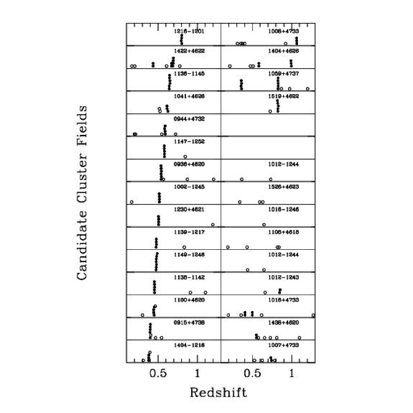
Figure 1.— The redshift distribution of galaxies in all cluster fields observed with LRIS on Keck. Each panel represents the results for one candidate cluster field. Each circle represents one galaxy redshift. Filled circles represent galaxies within 1000 km sec^-1 of another galaxy. Circles are stacked vertically within each panel to avoid overlap in the Figure. The two empty panels do not represent candidate cluster fields.

Figure 2.— upper panel: The derived BCG magnitude observed in the $W$ filter, m_W, vs. $z_{spec}$ for clusters from our survey (filled circles) and three known low redshift clusters that fall in our cluster survey area and have redshifts published in the literature (open circles). Error bars represent the photometric errors and errors due to the surface brightness correction term, summed in quadrature. The solid line is our parameterization of this relation (see text for details). lower panel: Comparison of $z_{spec}$ vs. $z_{BCG}$. The line is the expected 1:1 correlation of $z_{spec}$ and $z_{BCG}$. The data have an rms dispersion of 0.05.

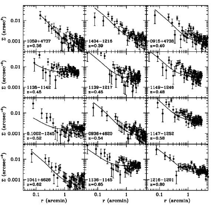
Figure 3.— The surface number density profiles for our spectroscopically confirmed clusters with $I$-band luminosity functions. All galaxies within 700 pixels of the cluster center are considered. We fit the profiles with a radial profile of the form $C_{1}+C_{2}/(1+r)^{2}$ (solid lines).

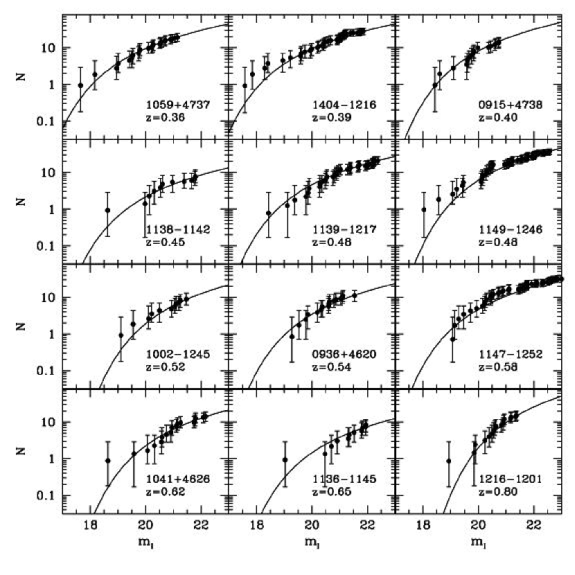
Figure 4.— The cumulative number of galaxies as a function of magnitude for our spectroscopically confirmed clusters with $I$-band data. Overlaid is the best fitting Schechter function (solid line).

Figure 5.— upper panel: The derived value of m${}^{*}_{I}$ vs. $z_{spec}$ for clusters from our survey, A93, S97, and SED98. The line is a linear fit to the data. The error bars are $\sigma_{mean}$ for clusters binned in $\Delta z=0.1$, where the mean is taken to be the value of the fit corresponding to the center of the redshift bin. lower panel: Comparison of $z_{lum}$ vs. $z_{spec}$. The line is the expected 1:1 correlation between the two redshifts indicators and has an rms dispersion of 0.06.

Figure 6.— upper panel: The location of the red envelope in ($V-I$) vs. $z_{spec}$ for clusters from our survey, A93, S97, and SED98. Error bars are $\sigma_{mean}$ for clusters binned in $\Delta z=0.1$, where the mean is taken to be the value of the fit corresponding to the center of the redshift bin. lower panel: Comparison of $z_{spec}$ vs. $z_{col}$. The line is the expected correlation of $z_{spec}$ and $z_{col}$ and has an rms dispersion of 0.07.

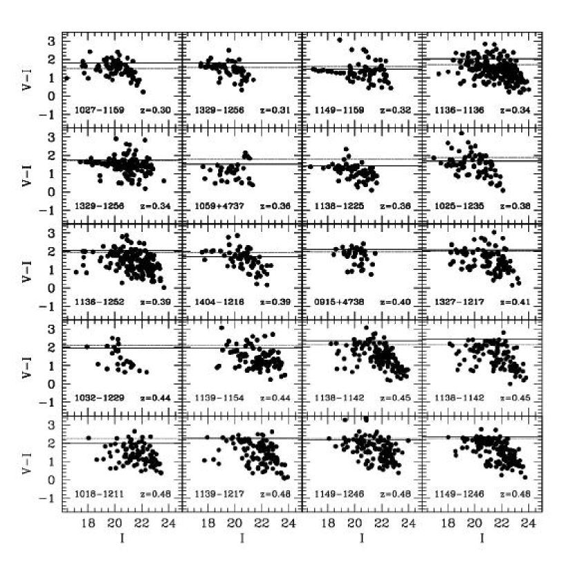
Figure 7.— Optical color magnitude diagrams for our clusters, ordered in increasing redshift ($z_{lum}$ is used if $z_{spec}$ does not exist). Solid lines are the location of the red envelope as determined by our automated procedure (see text for details). The dashed line corresponds to the expected location of the red envelope based on the cluster’s redshift and our $(V-I)$ vs. $z$ relation.

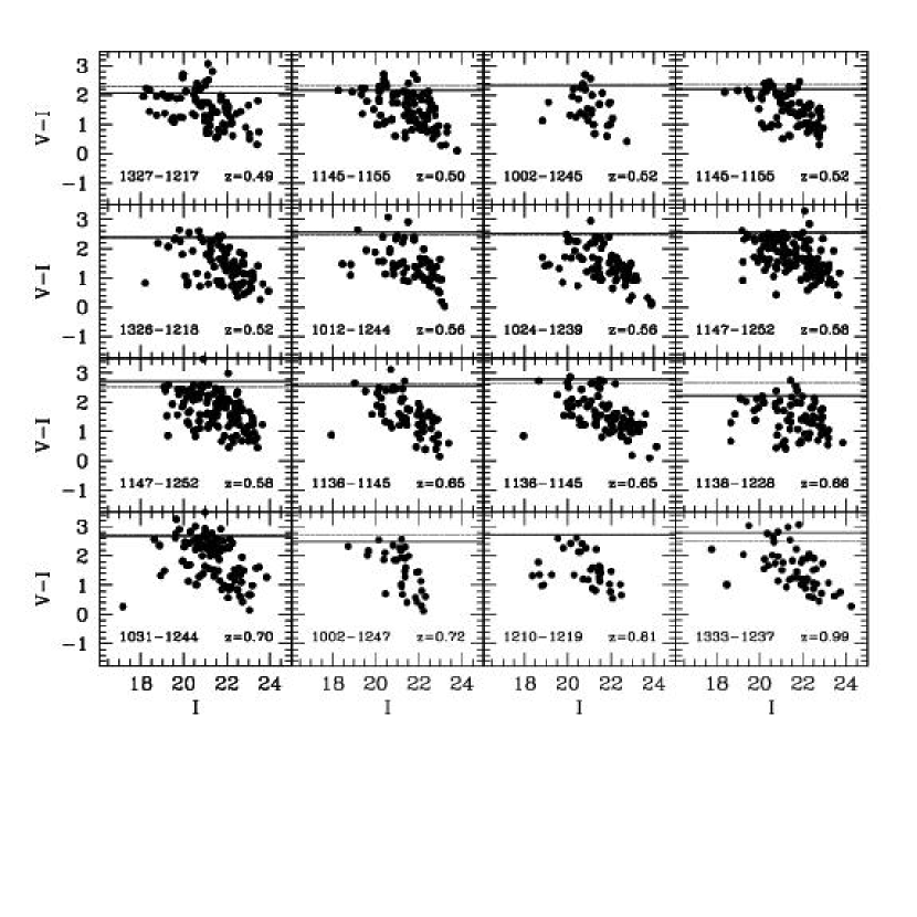
Figure 7.— continued.

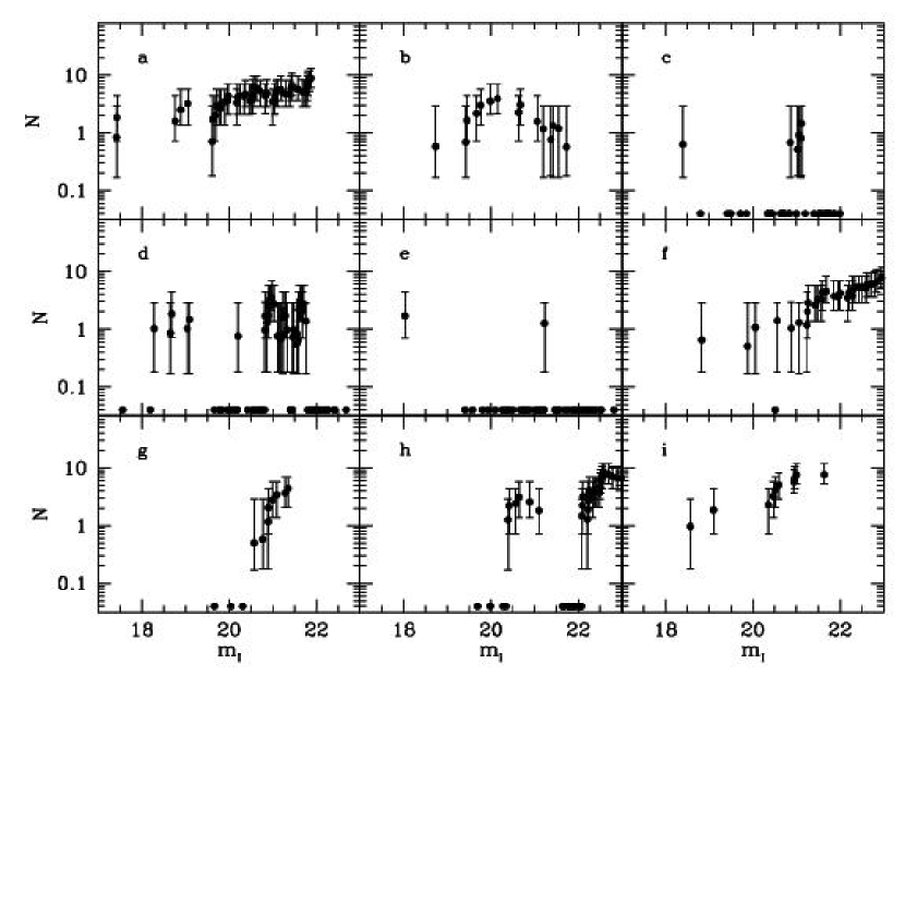
Figure 8.— Cumulative luminosity functions for random fields on our images (panels a-f) and non-cluster detections (panels g-i). See text for details.

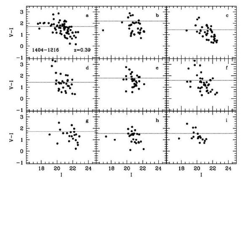
Figure 9.— Color-magnitude diagrams for random fields on our images (panels b-f) and non-cluster detections (panels g-i). We reproduce the CM diagram of cluster 1404$-$1216, a spectroscopically confirmed cluster at $z=0.39$, for reference (panel a). The location of the maximum change in the number of galaxies as a function of redshift as determined by our automated routine is indicated by solid lines.

Figure 10.— Comparison of the estimated redshifts derived using the three photometric redshift estimation techniques, $z_{lum}$, $z_{col}$, and $z_{BCG}$.

Figure 11.— left panel: The redshift dependence of M${}^{*}_{I}$ vs. $z$ (in the observed $I$ frame) for our clusters with spectroscopic and photometric redshifts. Also included are clusters from A93, S97, and SED98. Error bars are $\sigma_{mean}$ for clusters binned in $\Delta z=0.1$, where the mean is taken to be the value of the fit corresponding to the center of the redshift bin. right panel: Comparison of our observed values of M${}^{*}_{I}$ with the expected luminosity evolution of both an elliptical (upper) and spiral (lower) galaxy using spectral synthesis models from Bruzual & Charlot (1993). The data are binned in $\Delta z=$0.1 and have errors bars which are $\sigma_{mean}$ of the binned data. Both no evolution and passive evolution models are considered. The models are normalized at $z=$0.45 which corresponds to the center of the redshift bin with the greatest number of spectroscopically confirmed clusters.

Figure 12.— Comparison between the observational limiting magnitude and the measured m_∗.

Figure 13.— left panel: The location of the red envelope in $V-I$ vs. $z$ for our clusters with spectroscopic and photometric redshifts. Also included are clusters from A93, S97, and SED98. Error bars are $\sigma_{mean}$ for clusters binned in $\Delta z=0.1$, where the mean is taken to be the value of the fit corresponding to the center of the redshift bin. right panel: Comparison of the observed location of the red envelope in $V-I$ with the expected color evolution of an elliptical galaxy using spectral synthesis models from Bruzual & Charlot (1993). The data are binned in $\Delta z=0.1$ and have errors bars which are $\sigma_{mean}$ of the binned data. Both no evolution and passive evolution models are considered.

Figure 14.— left panel: The location of the red envelope in $I-$$K^{\prime}$ vs. $z$ for our clusters with spectroscopic and photometric redshifts. Also included are clusters from A93 and SED98. Error bars are $\sigma_{mean}$ for clusters binned in $\Delta z=0.1$, where the mean is taken to be the value of the fit corresponding to the center of the redshift bin. right panel: Comparison of the observed location of the red envelope in $I-$$K^{\prime}$ with the expected color evolution of an elliptical galaxy using spectral synthesis models from Bruzual & Charlot (1993). The data are binned in $\Delta z=0.1$ and have errors bars which are $\sigma_{mean}$ of the binned data. Both no evolution and passive evolution models are considered.

Figure 15.— The peak surface brightness of the cluster detection, $\Sigma(1+z)^{4}$, compared to (M${}^{*}_{I}$ $+5\log h)$ (left panel) and the location of the red envelope in $(V-I)$ (right panel). The values of L_x are inferred from our empirically determined correlation between $\Sigma(1+z)^{4}$ and L_x; they are not directly observed. Neither of the galaxy properties are significantly correlated with $\Sigma(1+z)^{4}$ according to the Spearman rank test.

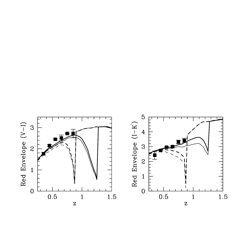
Figure 16.— The observed location of the red envelope in $V-I$ (left panel) and $I-$$K^{\prime}$ (right panel) compared to spectral synthesis models of Bruzual & Charlot (1993) for a passively evolving elliptical galaxy that includes a secondary burst of star formation. The data are binned in redshift intervals of $\Delta z=0.1$ and have errors bars which are $\sigma_{mean}$ of the binned data. In all models, the elliptical forms at $z_{form}=10$ and passively evolves until experiencing a secondary burst of star formation at $z_{burst}=1.5$ (solid lines) or $z_{burst}=1$ (dashed lines). We investigate burst strengths (the percentage of the galaxy’s mass that is converted into stars) of 10% (thick lines) and 25% (thin lines).

Table 1Observations

	RA	DEC	V	Seeing	I	Seeing	K′	Seeing
Cluster	(JD2000)	(JD2000)	(min)	(′′)	(min)	(′′)	(min)	(′′)
0915+4738	09:15:51.94	+47:38:19.9	50	1.8	33	1.9	56	2.0
0936+4620	09:36:06.28	+46:20:43.2	80	2.5	80	1.9	64	2.0
0944+4732	09:44:21.83	+47:32:42.6	…	…	…	…	40	2.0
1002$-$1245	10:02:01.47	$-$12:45:35.1	120	1.4	60	1.4	…	…
1002$-$1247	10:02:27.14	$-$12:47:13.1	120	1.4	60	1.4	…	…
1005$-$1147	10:05:43.60	$-$11:47:43.1	…	…	60	1.2	…	…
1005$-$1209	10:05:49.72	$-$12:09:36.5	…	…	45	1.4	…	…
1006$-$1222	10:06:29.25	$-$12:22:13.7	…	…	45	1.4	…	…
1006$-$1258	10:06:18.79	$-$12:58:12.5	…	…	68	1.1	…	…
1007$-$1208	10:07:42.60	$-$12:08:36.0	…	…	40	1.3	…	…
1012$-$1243	10:12:14.58	$-$12:43:10.9	…	…	45	0.8	32	0.8
1012$-$1245	10:12:44.35	$-$12:45:37.9	30	0.9	30	0.7	…	…
1014$-$1143	10:14:56.31	$-$11:43:08.1	…	…	45	1.2	…	…
1015$-$1132	10:15:19.47	$-$11:32:55.5	…	…	60	1.3	…	…
1017$-$1128	10:17:45.31	$-$11:28:07.8	…	…	60	1.1	…	…
1018$-$1211	10:18:46.45	$-$12:11:52.8	40	1.2	40	0.6	…	…
1023$-$1303	10:23:10.11	$-$13:03:52.0	…	…	30	0.6	…	…
1024$-$1239	10:24:44.94	$-$12:39:55.6	40	1.1	40	0.9	…	…
1025$-$1236	10:25:08.83	$-$12:36:20.0	90	1.5	115	2.7	…	…
1027$-$1159	10:27:26.31	$-$11:59:33.6	90	1.5	105	1.8	…	…
1031$-$1244	10:31:50.26	$-$12:44:27.2	40	1.0	60	0.8	…	…
1032$-$1229	10:32:04.91	$-$12:29:43.8	120	1.8	115	1.8	…	…
…	…	…	…	…	15	1.0	…	…
1041+4626	10:41:03.79	+46:26:36.3	40	2.5	60	2.2	118	2.0
1059+4737	10:59:38.03	+47:37:38.6	50	3.3	50	2.0	55	2.0
1100+4620	11:00:57.36	+46:20:38.3	…	…	…	…	88	2.0
1136$-$1136	11:36:31.95	$-$11:36:07.7	30	1.3	30	1.1	…	…
…	…	…	…	…	20	1.1	…	…
1136$-$1145	11:36:47.07	$-$11:45:33.3	13	1.1	20	0.9	44	0.8
…	…	…	40	1.0	40	0.8	…	…
1136$-$1252	11:36:33.54	$-$12:52:03.3	20	0.8	20	0.6	20	2.0
…	…	…	…	…	20	1.4	…	…
1138$-$1142	11:38:06.59	$-$11:42:10.3	20	1.1	30	0.7	32	0.8
…	…	…	60	1.3	60	1.2	…	…
1138$-$1225	11:38:14.24	$-$12:25:53.9	90	1.2	120	2.0	…	…
1138$-$1228	11:38:44.70	$-$12:28:25.4	30	0.7	20	0.8	…	…
1139$-$1154	11:39:30.47	$-$11:54:25.0	30	0.9	30	0.8	10	2.0
1139$-$1217	11:39:56.84	$-$12:17:19.8	20	0.7	20	0.8	32	0.8
1145$-$1155	11:45:22.36	$-$11:55:52.1	20	0.7	20	1.0	50	2.0
…	…	…	40	1.2	30	0.8	…	…
1147$-$1252	11:47:16.98	$-$12:52:04.7	20	1.0	20	0.9	32	0.8
…	…	…	40	1.2	30	0.7	…	…
1149$-$1159	11:49:22.14	$-$11:59:19.3	3	0.9	10	0.9	…	…
1149$-$1246	11:49:06.18	$-$12:46:06.3	20	0.9	20	0.8	32	0.8
…	…	…	40	1.0	40	0.7	…	…
1208$-$1151	12:08:26.67	$-$11:51:25.6	90	1.4	68	1.2	…	…
1210$-$1219	12:10:12.73	$-$12:19:06.9	60	1.4	60	1.4	…	…

Table 1Observations: Continued

	RA	DEC	V	Seeing	I	Seeing	K′	Seeing
Cluster	(JD2000)	(JD2000)	(min)	(′′)	(min)	(′′)	(min)	(′′)
1211$-$1220	12:11:04.16	$-$12:20:47.7	…	…	45	0.8	…	…
1215$-$1252	12:15:41.08	$-$12:52:59.7	…	…	68	1.1	…	…
1216$-$1201	12:16:45.10	$-$12:01:17.3	…	…	45	1.3	…	…
1219$-$1154	12:19:34.88	$-$11:54:22.9	…	…	60	1.3	…	…
1219$-$1201	12:19:44.49	$-$12:01:35.5	…	…	60	1.3	…	…
1221$-$1206	12:21:46.20	$-$12:06:12.7	…	…	45	1.2	…	…
1230+4621	12:30:16.26	+46:21:17.1	67	3.8	33	2.2	72	2.0
1326$-$1218	13:26:12.66	$-$12:18:22.5	40	0.9	50	0.9	36	0.8
1327$-$1217	13:27:57.33	$-$12:17:16.7	20	1.1	20	1.0	42	0.8
…	…	…	40	1.3	50	0.8	…	…
1329$-$1256	13:29:11.37	$-$12:56:22.0	90	1.6	95	1.4	20	2.0
…	…	…	45	1.1	30	1.0	…	…
1333$-$1237	13:33:01.92	$-$12:37:17.0	20	0.9	30	1.2	…	…
1404$-$1216	14:04:47.20	$-$12:16:21.4	90	1.5	60	1.3	…	…
1405$-$1147	14:05:11.38	$-$11:47:08.6	…	…	60	1.4	…	…
1406$-$1232	14:06:36.54	$-$12:32:39.7	…	…	45	1.4	…	…
1408$-$1209	14:08:17.86	$-$12:09:27.0	…	…	68	1.0	…	…
1408$-$1216	14:08:45.95	$-$12:16:08.8	…	…	68	1.0	…	…
1408$-$1218	14:08:50.62	$-$12:18:14.8	…	…	68	1.0	…	…
1412$-$1150	14:12:32.56	$-$11:50:16.2	…	…	8	1.2	…	…
…	…	…	…	…	30	0.8	…	…
1412$-$1222	14:12:25.92	$-$12:22:53.3	…	…	8	1.3	…	…
…	…	…	…	…	45	0.8	…	…
1412$-$1222.1	14:12:31.26	$-$12:22:15.8	…	…	45	0.8	…	…
1413$-$1244	14:13:08.59	$-$12:44:11.6	…	…	40	1.2	…	…
1416$-$1143	14:16:45.13	$-$11:43:40.0	…	…	40	1.3	…	…
1422+4622	14:22:24.18	+46:22:39.7	80	1.7	83	2.4	35	2.0
1519+4622	15:19:54.27	+46:22:20.4	…	…	15	2.3	45	2.0

Table 2Redshift Data

Cluster	zspec	zlum	$\sigma_{z_{lum}}$	zcol	$\sigma_{z_{col}}$	zbcg	$\sigma_{z_{bcg}}$	m${}^{*}_{I}$	$\sigma_{m^{*}_{I}}$	V$-$I	$\sigma_{V-I}$	I$-$K	$\sigma_{I-K}$
0915+4738	0.40	0.43	0.06	0.50	0.07	…	…	18.77	0.08	2.12	0.05	2.88	0.03
0936+4620	0.54	0.49	0.06	…	…	…	…	18.97	0.08	…	…	2.96	0.03
0944+4732	0.58	…	…	…	…	…	…	…	…	…	…	…	…
1002$-$1245	0.52	0.64	0.06	0.50	0.07	0.43	0.05	19.65	0.11	2.32	0.03	…	…
1002$-$1247	…	0.72	0.06	0.55	0.07	0.57	0.05	19.82	0.14	2.48	0.03	…	…
1005$-$1147	…	0.89	0.06	…	…	0.53	0.05	20.24	0.21	…	…	…	…
1005$-$1209	…	0.45	0.06	…	…	…	…	18.82	0.08	…	…	…	…
1006$-$1222	…	1.01	0.06	…	…	0.72	0.05	20.54	0.21	…	…	…	…
1006$-$1258	…	0.73	0.06	…	…	0.47	0.05	19.88	0.14	…	…	…	…
1007$-$1208	…	0.49	0.06	…	…	0.41	0.05	18.99	0.08	…	…	…	…
1012$-$1243	…	0.49	0.06	…	…	0.44	0.05	18.99	0.08	…	…	…	…
1012$-$1245	…	0.56	0.06	0.59	0.07	…	…	19.28	0.07	2.56	0.07	…	…
1014$-$1143	…	0.30	0.06	…	…	…	…	17.95	0.12	…	…	…	…
1015$-$1132	…	0.60	0.06	…	…	0.45	0.05	19.43	0.07	…	…	…	…
1017$-$1128	…	0.50	0.06	…	…	0.66	0.05	19.04	0.08	…	…	…	…
1018$-$1211	…	0.48	0.06	0.41	0.07	0.47	0.05	18.94	0.08	2.00	0.07	…	…
1023$-$1303	…	0.51	0.06	…	…	0.77	0.05	19.10	0.07	…	…	…	…
1024$-$1239	…	0.56	0.06	0.57	0.07	0.76	0.05	19.28	0.07	2.52	0.03	…	…
1025$-$1236	…	0.38	0.06	0.35	0.07	0.34	0.05	18.48	0.12	1.68	0.07	…	…
1027$-$1159	…	0.30	0.06	0.37	0.07	0.37	0.05	17.95	0.12	1.80	0.07	…	…
1031$-$1244	…	0.70	0.06	0.65	0.07	0.70	0.05	19.76	0.11	2.68	0.07	…	…
1032$-$1229	…	0.44	0.06	0.41	0.07	0.45	0.05	18.76	0.08	1.96	0.07	…	…
	…	0.50	0.06	…	…	…	…	19.04	0.08	…	…	…	…
1041+4626	0.62	0.61	0.06	…	…	…	…	19.45	0.11	…	…	3.04	0.07
1059+4737	0.36	0.33	0.06	0.28	0.07	…	…	18.18	0.12	1.52	0.07	3.00	0.07
1100+4620	0.46	…	…	…	…	…	…	…	…	…	…	…	…
1136$-$1136	…	0.34	0.06	0.42	0.07	…	…	18.20	0.12	2.04	0.05	…	…
	…	0.34	0.06	…	…	…	…	18.24	0.12	…	…	…	…
1136$-$1145	0.65	0.59	0.06	0.59	0.07	0.67	0.05	19.31	0.07	2.56	0.07	2.92	0.03
	…	0.67	0.06	0.77	0.07	…	…	19.68	0.11	2.80	0.21	2.96	0.03
1136$-$1252	…	0.39	0.06	0.42	0.07	0.37	0.05	18.49	0.12	2.04	0.05	…	…
	…	0.31	0.06	…	…	…	…	18.00	0.12	…	…	…	…
1138$-$1142	0.45	0.45	0.06	0.51	0.07	0.52	0.05	18.81	0.08	2.36	0.03	2.72	0.04
	…	0.46	0.06	0.54	0.07	…	…	18.86	0.08	2.44	0.03	…	…
1138$-$1225	…	0.36	0.06	0.30	0.07	0.36	0.05	18.34	0.12	1.44	0.07	…	…
1138$-$1228	…	0.66	0.06	0.48	0.07	…	…	19.63	0.11	2.24	0.05	…	…
1139$-$1154	…	0.44	0.06	0.41	0.07	…	…	18.76	0.08	1.96	0.07	…	…
1139$-$1217	0.48	0.44	0.06	0.49	0.07	…	…	18.70	0.12	2.28	0.05	2.72	0.04
1145$-$1155	…	0.52	0.06	0.47	0.07	0.44	0.05	19.13	0.07	2.20	0.05	…	…
	…	0.50	0.06	0.45	0.07	…	…	19.04	0.08	2.16	0.05	…	…
1147$-$1252	0.58	0.53	0.06	0.59	0.07	0.62	0.05	19.05	0.08	2.56	0.07	2.92	0.03
	…	0.49	0.06	0.69	0.07	…	…	18.93	0.08	2.72	0.03	3.00	0.07
1149$-$1159	…	0.32	0.06	0.31	0.07	0.23	0.05	18.09	0.12	1.48	0.07	…	…
1149$-$1246	0.48	0.45	0.06	0.47	0.07	0.48	0.05	18.85	0.08	2.20	0.05	2.72	0.04
	…	0.52	0.06	0.51	0.07	…	…	19.15	0.07	2.36	0.03	2.76	0.04
1208$-$1151	…	0.61	0.06	…	…	…	…	19.47	0.11	…	…	…	…

Table 2Redshift Data: Continued

Cluster	zspec	zlum	$\sigma_{z_{lum}}$	zcol	$\sigma_{z_{col}}$	zbcg	$\sigma_{z_{bcg}}$	m${}^{*}_{I}$	$\sigma_{m^{*}_{I}}$	V$-$I	$\sigma_{V-I}$	I$-$K	$\sigma_{I-K}$
1210$-$1219	…	0.81	0.06	0.68	0.07	0.74	0.05	20.06	0.14	2.72	0.03	…	…
1211$-$1220	…	0.89	0.06	…	…	0.52	0.05	20.24	0.21	…	…	…	…
1215$-$1252	…	0.39	0.06	…	…	…	…	18.49	0.12	…	…	…	…
1216$-$1201	0.80	0.92	0.06	…	…	0.80	0.05	20.33	0.21	…	…	…	…
1219$-$1154	…	0.83	0.06	…	…	0.68	0.05	20.13	0.14	…	…	…	…
1219$-$1201	…	0.56	0.06	…	…	0.55	0.05	19.28	0.07	…	…	…	…
1221$-$1206	…	0.34	0.06	…	…	…	…	18.20	0.12	…	…	…	…
1230+4621	0.51	…	…	…	…	…	…	…	…	…	…	3.08	0.21
1326$-$1218	…	0.52	0.06	0.53	0.07	…	…	19.12	0.07	2.40	0.03	2.72	0.04
1327$-$1217	…	0.41	0.06	0.43	0.07	…	…	18.60	0.12	2.08	0.05	2.80	0.04
	…	0.49	0.06	0.43	0.07	…	…	18.99	0.08	2.08	0.05	2.56	0.29
1329$-$1256	…	0.31	0.06	0.37	0.07	0.37	0.05	18.00	0.12	1.80	0.07	2.16	0.29
	…	0.34	0.06	0.36	0.07	…	…	18.20	0.12	1.76	0.07	2.12	0.29
1333$-$1237	…	0.99	0.06	0.77	0.07	…	…	20.50	0.21	2.80	0.21	…	…
1404$-$1216	0.39	0.34	0.06	0.35	0.07	0.47	0.05	18.28	0.12	1.72	0.07	…	…
1405$-$1147	…	0.96	0.06	…	…	0.64	0.05	20.42	0.21	…	…	…	…
1406$-$1232	…	0.96	0.06	…	…	…	…	20.43	0.21	…	…	…	…
1408$-$1209	…	0.34	0.06	…	…	0.48	0.05	18.19	0.12	…	…	…	…
1408$-$1216	…	0.60	0.06	…	…	…	…	19.43	0.07	…	…	…	…
1408$-$1218	…	0.60	0.06	…	…	0.55	0.05	19.43	0.07	…	…	…	…
1412$-$1150	…	0.66	0.06	…	…	0.71	0.05	19.63	0.11	…	…	…	…
	…	0.75	0.06	…	…	…	…	19.90	0.14	…	…	…	…
1412$-$1222	…	0.32	0.06	…	…	…	…	18.09	0.12	…	…	…	…
	…	0.31	0.06	…	…	…	…	18.00	0.12	…	…	…	…
1412$-$1222.1	…	0.58	0.06	…	…	…	…	19.32	0.07	…	…	…	…
1413$-$1244	…	0.81	0.06	…	…	0.63	0.05	20.06	0.14	…	…	…	…
1416$-$1143	…	0.54	0.06	…	…	…	…	19.20	0.07	…	…	…	…
1422+4622	0.69	…	…	0.32	…	…	…	…	…	1.56	…	…	…
1519+4622	0.82	…	…	…	…	…	…	…	…	…	…	…	…

Table 3Evolution Parametrizations

	Functional
Type	Form	Coefficients
Luminosity	(M${}^{*}_{I}+5\log h)={\rm C_{1}}+{\rm C_{2}}z$	C${}_{1}=-21.70\pm 0.04$
		C${}_{2}=-0.94\pm 0.09$
Color ($V-I$)	($V-I)~{}=~{}$C${}_{1}+$ C${}_{2}z~{}+~{}$C${}_{3}z^{2}$	C${}_{1}=-0.02\pm 0.11$
		C${}_{2}=6.73\pm 0.41$
		C${}_{3}=-4.09\pm 0.35$
Color ($I-K^{\prime})$	($I-K^{\prime})~{}=~{}$C${}_{1}~{}+~{}$C${}_{2}z~{}+~{}$C${}_{3}z^{2}~{}+~{}$C${}_{4}z^{3}$	C${}_{1}=-0.50\pm 0.76$
		C${}_{2}=15.1\pm 4.1$
		C${}_{3}=-23.2\pm 7.2$
		C${}_{4}=12.6\pm 4.2$

References

- a (96) Abraham, R.G., et al. 1996, ApJ, 471, 694
- a (99) Andreon, S., & Ettori, S. 1999, ApJ, 516, 647
- a (98) Aragon-Salamanca, A., Baugh, C.M., & Kauffmann, G. 1998, MNRAS, 297, 427
- a (93) Aragon-Salamanca, A., Ellis, R.S., Couch, W.J., & Carter, D. 1993, MNRAS, 262, 764 (A93)
- b (96) Barrientos, L.F., Schade, D., & Lopez-Cruz, O. 1996, ApJ, 460, L89
- bx (96) Bender, R., Ziegler, B., & Bruzual, G. 1996, ApJ, 463, L51
- by (96) Bertin, E. & Arnouts, S. 1996, A&AS, 117, 393
- b (92) Bower, R.G., Lucey, J.R., & Ellis, R.S. 1992, MNRAS, 254, 601
- b (93) Bruzual, G. & Charlot, S. 1993, ApJ, 405, 538
- b (84) Butcher, H. & Oemler, A. 1984, ApJ, 285, 426 (B-O)
- c (00) Cohen, J.G. et al. 2000, ApJ, 538, 29
- c (98) Collins, C.A., & Mann, R.G. 1998, MNRAS, 297, 128
- cx (98) Couch, W.J., Barger, A.J., Smail, I., Ellis, R.S., & Sharples, R.M. 1998, ApJ, 497, 188
- c (91) Couch, W.J., Ellis, R.S., MacLaren, I., & Malin, D. 1991, MNRAS, 249, 606 (C91)
- c (94) Couch, W.J., Ellis, R.S., Sharples, R.M., & Smail, I. 1994, ApJ, 430, 121
- c (87) Couch, W.J., & Sharples, R.M. 1987, MNRAS, 229, 423
- d (96) Dalcanton, J.J. 1996, ApJ, 466, 92
- d (97) Dalcanton, J.J., Spergel, D.N., Gunn, J.E., Schmidt, M., & Schneider, D.P. 1997, AJ, 114, 635
- dx (99) de Propris, R., Stanford, S.A., Eisenhardt, P.R., Dickinson, M., & Elston, R. 1999, AJ, 118, 719
- d (82) Dressler, A., & Gunn, J.E. 1982, ApJ, 263, 533
- d (83) Dressler, A., & Gunn, J.E. 1983, ApJ, 270, 7
- d (92) Dressler, A., & Gunn, J.E. 1992, ApJS, 78, 1
- d (94) Dressler, A., Oemler, A., Butcher, H., & Gunn, J.E. 1994, ApJ, 430, 107
- d (99) Dressler, A., Smail, I., Poggianti, B.M., Butcher, H., Couch, W.J., Ellis, R.S., & Oemler, A. 1999, ApJS, 122, 51
- e (97) Ellis, R.S., Smail, I., Dressler, A., Couch, W.J., Oemler, A., Jr., Butcher, H., & Sharples, R.M. 1997, ApJ, 483, 582
- f (98) Fisher, D., Fabricant, D., Franx, M., & van Dokkum, P. 1998, ApJ, 498, 195
- f (95) Fukugita, M., Shimasaku, K., & Ichikawa, T. 1995, PASP, 107, 945
- gr (99) Garilli, B., Maccagni, D., & Anfreon, S. 1999, å, 342, 408
- g (00) Gonzalez, A.H., Zaritsky, D., Dalcanton, J.J., & Nelson, A.E. 2001, ApJS, in press
- g (87) Gunn, J.E. et al. 1987, Opt. Eng., 26, 779
- g (86) Gunn, J.E., Hoessel, J.G., & Oke, J.B. 1986, ApJ, 306, 30 (GHO)
- gu (97) Guzman, R., et al. 1997, ApJ, 489, 559
- h (80) Hoessel, J.G 1980, ApJ, 241, 493
- hx (80) Hoessel, J.G., Gunn, J.E., & Thuan, T.X. 1980, ApJ, 241, 486
- j (00) Jones, L., Smail, I., & Couch, W.J. 2000, ApJ, 528, 118
- ky (98) Kauffmann, G., & Charlot, S. 1998, MNRAS, 297, L23
- k (00) Kelson, D.D., Illingworth, G.D., van Dokkum, P.G., & Franx, M. 2000, ApJ, 531, 184
- k (01) Kelson, D.D., Illingworth, G.D., Franx, M., & van Dokkum, P.G. 2001, ApJ, 552, L17
- k (97) Kelson, D.D., van Dokkum, P., Franx, M., Illingworth, G.D., & Fabricant, D. 1997, ApJ, 478, L13
- k (98) Kodama, T., Arimoto, N., Barger, A.J., & Aragon-Salamanca, A. 1998, A&A, 334, 99
- kx (01) Kodama, T. & Bower, R.G. 2001, MNRAS, 321, 18
- l (83) Landolt, A.U. 1983, AJ, 88, 439
- l (92) Landolt, A.U. 1992, AJ, 104, 340
- lx (92) Lauer, T.R. & Postman, M. 1992, ApJ, 400, L47
- lo (97) Lowenthal, J.D., et al. 1997, ApJ, 481, 673
- l (86) Lugger, P. 1986, ApJ, 303, 535
- l (96) Lubin, L.M. 1996, AJ, 112, 23
- n (00) Nelson, A.E., Gonzalez, A.H., Zaritsky, D., & Dalcanton, J.J. 2000 ApJ, in prep
- o (88) O’Connell, R., 1988, in Towards Understanding Galaxies at High Redshift, ed. Dordrecht (Erice: Kluwer Academic Publishers), 177
- o (97) Oemler, A., Dressler, A., & Butcher, H. 1997, ApJ, 474, 561
- o (95) Oke, J., et al. 1995, SPIE, 2198, 178
- p (98) Persson, S.E., Murphy, D.C., Krzeminski, W., Roth, M., & Rieke, M.J. 1998, AJ, 116, 2475
- p (97) Phillips, A.C. et al. 1997, ApJ, 489, 543
- p (99) Poggianti, B.M., Smail, I., Dressler, A., Couch, W.J., Barger, A.J., Butcher, H., Ellis, R.S., & Oemler, A. 1999, ApJ, 518, 576
- p (95) Postman, M. & Lauer, T.R. 1995, ApJ, 440, 28
- p (96) Postman, M., Lubin, L.M., Gunn, J.E., Oke, J.B., Hoessel, J.G., Schneider, D.P., & Christensen, J.A. 1996, AJ, 111, 615
- r (95) Rakos, K.D., & Schombert, J.M. 1995, ApJ, 439, 47 (RS)
- s (73) Sandage, A. & Hardy, E. 1973, ApJ, 183, 743
- s (76) Schechter, P. 1976, ApJ, 203, 297
- sy (98) Schlegel, D.J., Finkbeiner, D.P., & Davis, M. 1998, ApJ, 500, 525
- s (83) Schneider, D.P., Gunn, J.E., & Hoessel, J.G. 1983a, ApJ, 264, 337
- sx (83) Schneider, D.P., Gunn, J.E., & Hoessel, J.G. 1983b, ApJ, 268, 476
- s (94) Schneider, D.P., Schmidt, M., & Gunn, J.E. 1994, AJ, 107, 124
- s (96) Shectman, S.A., Landy, S.D., Oemler, A., Tucker, D.L., Lin, H., Kirshner, R.P., Schechter, P.L. 1996, ApJ, 470, 172
- s (97) Smail, I., Dressler, A., Couch, W.J., Ellis, R.S., Oemler, A., Butcher, H., & Sharples, R.M. 1997, ApJS, 110, 213 (S97)
- s (98) Smail, I., Edge, A.C., Ellis, R.S., & Blandford, R.D. 1998, MNRAS, 293, 124
- s (95) Stanford, S.A., Eisenhardt, P.R., & Dickinson, M. 1995, ApJ, 450, 512
- sx (98) Stanford, S.A., Eisenhardt, P.R., & Dickinson, M. 1998, ApJ, 492, 461 (SED98)
- v (01) van Dokkum, P. G. & Franx, M. 2001, ApJ, 553, 90
- v (99) van Dokkum, P.G., Franx, M., Fabricant, D., Kelson, D.D., & Illingworth, G.D. 1999, ApJ, 520, L95
- v (98) van Dokkum, P.G., Franx, M., Kelson, D.D., Illingworth, G.D.I., Fisher, D., & Fabricant, D. 1998, ApJ, 500, 714
- v (97) Vogt, N.P., et al. 1997, ApJ, 479, L121
- z (97) Zaritsky, D., Nelson, A.E., Dalcanton, J.J., & Gonzalez, A.H. 1997, ApJ, 480, L91
- z (96) Zaritsky, D., Shectman, S.A., & Bredthauer, G. 1996, PASP, 108, 104