Very high-energy $\gamma$-ray observations of the Crab nebula and other potential sources with the GRAAL experiment

Abstract

The “Gamma Ray Astronomy at ALmeria” (GRAAL) experiment uses 63 heliostat-mirrors with a total mirror area of $\approx$ 2500 m² from the CESA-1 field at the “Plataforma Solar de Almeria” (PSA) to collect Cherenkov light from air showers. The detector is located in a central solar tower and detects photon-induced showers with an energy threshold of 250 $\pm$ 110 GeV and an asymptotic effective detection area of about 15000 m². A comparison between the results of detailed Monte-Carlo simulations and data is presented.
Data sets taken in the period September 1999 - September 2000 in the direction of the Crab pulsar, the active galaxy 3C 454.3, the unidentified $\gamma$-ray source 3EG 1835+35 and a “pseudo source” were analyzed for high energy $\gamma$-ray emission. Evidence for a $\gamma$-ray flux from the Crab pulsar with an integral flux of 2.2 $\pm$ 0.4 (stat) ${}^{+1.7}_{-1.3}$ (syst) $\times$ 10^-9 cm^-2 sec^-1 above threshold and a significance of 4.5 $\sigma$ in a total measuring time of 7 hours and 10 minutes on source was found. No evidence for emission from the other sources was found.
Some difficulties with the use of heliostat fields for $\gamma$-ray astronomy are pointed out. In particular the effect of field-of-view restricted to the central part of a detected air shower on the lateral distribution and timing properties of Cherenkov light are discussed. Upon restriction the spread of the timing front of proton induced showers sharply decreases and the reconstructed direction becomes biased towards the pointing direction. This is shown to make efficient $\gamma$-hadron separation difficult.

1 Introduction - aims and plan of the paper

Measuring atmospheric Cherenkov radiation is presently the most effective way to detect cosmic $\gamma$-rays with primary energies between about 100 GeV and 1 TeV [1]. In order to reach low energy thresholds with techniques based on Cherenkov light, large mirror collection areas are needed. GRAAL is an experiment that employs the large mirror area of an existing tower solar-power plant for this purpose.
This paper briefly describes the GRAAL detector and reports results about the detection of $\gamma$-rays from cosmic sources. In addition some general lessons we learnt about the heliostat-field approach to $\gamma$-ray astronomy are reported. In section 2 the GRAAL detector is described and compared to other heliostat-field detectors for Cherenkov light. Section 3 describes the event reconstruction based mainly on the arrival time of signals at the central detector. Section 4 treats the Monte Carlo simulation of the experiment. Section 5 explains how the data set used for the analysis of this paper was chosen from the total set of all taken data. The data reduction procedures—and the fundamental problems besetting it—are explained in section 6 and the results are presented in section 7. Finally some concluding remarks are offered in section 8. A more detailed report about these results will be available in two theses[2, 3].

2 The GRAAL detector

2.1 The CESA-1 heliostat field at the PSA

CESA-1 is a heliostat field comprising of 300 steerable mirrors to the north of a central tower located within the “Plataforma Solar de Almeria”(PSA) a solar thermal-energy research centre operated by the Spanish CIEMAT. The PSA is located in the desert of Tabernas (37^∘.095 N, 2^∘.360 W) about 30 km from the city of Almeria and the sea, at the foothills of the Sierra-Nevada mountains (height a.s.l. of 505 m). The 63 heliostats used for GRAAL have a mirror area of 39.7 m² each and consist of 12 rectangular “facets” (sub mirrors) with a spherical curvature that are “canted” (adjusted relative to the overall frame) to a roughly spherical overall heliostat shape. The beam spread function of the heliostats has a RMS of about 0.25^∘. Each heliostat is individually steerable with stepping motors via a central PC. For the purpose of GRAAL a control program was developed that allowed to perform the special tracking needed for the use of the field for Cherenkov astronomy.
The heliostat focus the Cherenkov light of air showers from the direction of potential gamma-ray sources to software adjustable “aiming points” in the central tower (see fig.1). The so-called “convergent view”[4]—the pointing of the heliostats towards a point in the atmosphere corresponding to an atmospheric depth of 230 g/cm² in the general direction of the potential source of gamma rays—was always applied.
The relatively thin glass used for the heliostat mirrors (4 mm thickness) —leading to a low overall heat capacity—and the proximity of the ocean lead to frequent dew formation on the mirrors in the winter. To prevent micro drop formation, all mirrors were sprayed every second day with a tensid solution in the evening using a specially constructed spray cart. This procedure was found to work well after all mirrors had been cleand with sulfonic acid from traces of silicon gel—a common contaminant in glass production.

2.2 Detector setup

2.2.1 Secondary optics

Cherenkov light from four groups of heliostats (with 13,14,18,18 members, respectively) is directed onto four single non-imaging “cone concentrators” each containing a single large-area photomultiplier tube (PMT). The light collectors have the form of truncated Winston cones with an opening angle of 10^∘. Each cone has a front diameter 1.08 m and a length of 2.0 m. The cones are housed in a special enclosure that is fastened to the outside of the central tower at the 70 m level (see fig.2). Each cone is directed onto a point on the ground in the heliostat field and collects the light from all heliostats which are located within the ellipse projected by the cone opening angle on the ground (see fig. 3).
At the end of each cone, a six-stage 8 inch hemispherical PMT, optimized for operation under high background light levels (EMI 9352KB) is situated. The tubes were typically operated with about 1300 - 1600 V at a gain of about 8000. The signals were transmitted via AC coupling to one fast amplifier directly adjacent to the PMT and a second one near the data acquisition electronics within the tower. These amplifiers have a bandwidth of about 350 MHz and a gain of about 15 each. The final FWHM width of Cherenkov pulses is about 3.6 ns, and mainly determined by path length differences within the PMT.
The incoming light from an air shower consists of a train of pulses from the different heliostats, usually fully separated by pathlength differences. The arrival time and amplitude of each heliostat can thus be determined with a flash-ADC in a sequential mode (fig.4).

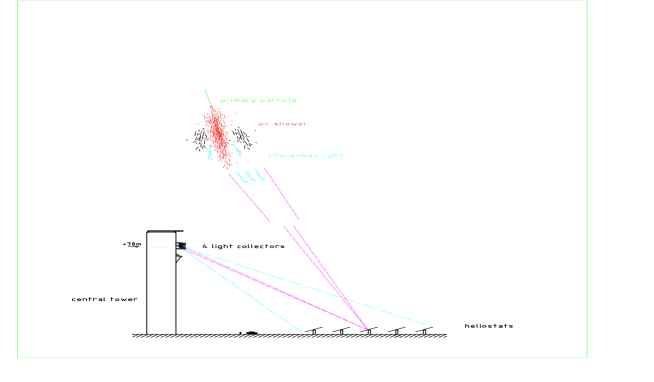
Figure 1: Scheme of the experiment seen from the side, north is to the right. The Cherenkov light of a schematic airshower (not to scale with respect to the field) is concentrated by the heliostats of the CESA-1 field to a focus at the central tower. A dedicated platform mounted at the outside of the tower at the 70 m level houses four Winston cones which receive light from 13 - 18 heliostats in the field. The data-acquisition electronics is located inside the tower.

Figure 2: Upper plot: Side view of the detector platform at the 70 m level of the central tower. Two of the four Winston cones pointing towards their respective heliostat subfields with the large-area PMTs at the ends are sketched. The wall of the central tower is at the left with a manhole to enter the platform. Lower plot: View from above, all four Cones are shown, the half circle is the wall of the central tower.

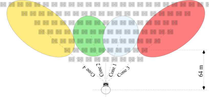
Figure 3: Scheme of the detection geometry seen from above, north is to the top of the page. The small circle is the tower, the tiled double square symbolize the heliostats of CESA-1 in the 2nd to 7th row from the tower. The light from one of the four groups of heliostats used in GRAAL - indicated by the ellipses - is concentrated into one of the four cones. The cone numbering indicated is used throughout the text.

Figure 4: The signal height in mV after amplification recorded in all four cones from one typical airshower is displayed as a function of time. The trigger occurs at 500 ns. The y-gain depends on amplitude, at 100 mV one mV corresponds to typically 0.25 photo electrons. Each peak corresponds to the Cherenkov-light flash of the shower reflected by a different heliostat. The distribution of light intensity on the ground within the field of view of the cones is very uneven, note the different y-scales.

2.2.2 Trigger logic

Two completely independent triggers are used. For the “sequence trigger” after a discriminated signal above 30 mV a gate of 40 ns length is opened after a delay of 20 ns. If a further signal is detected during gate duration, another gate of 40 ns is opened with a delay of 20 ns. If a third signal is detected in this second gate an event-trigger gate of 200 ns is opened. If the first and second cone have a coincident event-trigger the final event trigger is formed.
For the “charge(q) trigger” a timing-amplifier integrates the signal with an exponential time scale of 100 (200) ns for Cone 1+2 (3+4). The integrated signal is fed into a discriminator in all four cones and opens a coincidence gate of 200 ns duration if a preset threshold is surpassed (see also fig.16, where the Monte Carlo simulation of this trigger is discussed). The singles rate of this integrated signal is the “q-rate” (table 2 - 5). A majority coincidence requirement of “3 out of 4 cones” is required for the final event trigger.
Both triggers are always in a logical OR mode in data taking. The event rate of the “sequence trigger” depends sensitively on the incoming direction of the shower but is relatively insensitive on the level of night-sky background induced background light (NSB). The “charge trigger” is more strongly influenced by the NSB, but triggers on coincident signals independent of detailed hypotheses on the arrival-time structure.

2.2.3 Data readout

GRAAL achieves a good time resolution because there exist only four short cables that run exclusively within the platform enclosure from the photomultipliers to the data acquisition electronics. We register all four pulse trains in only one Digital Oscilloscope (Le Croy LC 564A) with a bandwidth of 1 GHz and a time bin of 500 ps. This ensures that the FWHM of individual pulses of about 3.6 ns is negligibly increased by electronics effects. The digital scope is read out in sequence mode over a GPIB interface into a PC, reaching a speed of about 260 “waveforms”/sec (i.e. 1000 time bins of 0.5 ns width with 1 byte each), which is sufficient for a dead time below 10 $\%$ for our master trigger rate which always remains below 5 Hz and is typically about 2-3 Hz (each trigger containing four waveforms).

2.2.4 Calibration

The time and amplitude calibration of our setup is performed using blue LEDs (Nichia NSPB 500, maximal output at 470 nm) with a calibrator module that is fastened at the window of the Winston cones. The amount of light emitted by the individual LEDs is determined with a Quantacon RCA C31000 (a photomuliplier yielding a well separated single photoelectron (p.e.) peak) that was previously calibrated by determining its single p.e. peak and fluctuation behaviour. The LED operating voltage is adjusted so that one LED pulse corresponds to about 100 p.e. These LED pulses are regularly used in each run to verify time and amplitude calibration. In addition a LED module with higher total light output shines onto the heliostat field. When the heliostats are brought into a “back reflection” position, the reflected LED pulses are used to verify the geometry and check the mirror quality.
The timing and gain properties of the electronics chain were calibrated on-line with a PC-controlled Phillips Scientific PS7120 charge injection module. Charge pulses with properties similar to PMT pulses and different amplitudes were injected directly after the PMT in each run.

2.2.5 Remote operation

All operations (like opening of the door, high-voltage control etc.) at the central receiver and the tracking of the heliostat field are under remote control via the internet. Various environmental parameters like humidity, ambient light, wind speed, rates etc. are checked by the data-acquisition computer. Under conditions that indicate some malfunction, a physicist on shift is phoned by the PC and can check all parameters and images of web cameras, remotely. For the operation of the heliostat field and emergencies only the regular night-operator of the PSA is on-site in all observation nights.

2.3 Differences of the basic “CELESTE” versus “GRAAL” central-receiver approach

After early tests for the use of heliostat fields for $\gamma$-ray astronomy [5] the basic idea of Tümer[6, 7] to image the Cherenkov light of one heliostat to a single photomultiplier has been worked out in technical detail in the proposal for the CELESTE experiment[4]. It was then proven technically at the Themis heliostat array [8]. Two other heliostat-field experiments “STACEE”[9, 10] and “Solar 2”[11] follow this basic design. Recently CELESTE[12] and STACEE[13] reported the detection of VHE $\gamma$ rays. The major differences between this well documented method to detect air showers with heliostat arrays and the “non-imaging” principle of GRAAL—which collects the light from 13-18 heliostats in a Winston cone onto a single large-area photomultiplier—are described in the following.
$\bullet$ The most important drawback of the non-imaging approach of GRAAL is that the night-sky background is higher roughly by the number of heliostats viewed by one cone. This results in a typical expected background of 8-10 p.e./ns in GRAAL, compared to 0.7 p.e./ns in CELESTE. The hardware energy threshold for the detection of $\gamma$-rays in principle achievable with the same mirror area used is about 4 times higher in GRAAL. For pulses far above threshold the performance of the two approaches is not expected to be very different because a similar amount of Cherenkov light is gathered by GRAAL and CELESTE.
$\bullet$ The advantage of the non-imaging approach is its greater simplicity leading to savings by about a factor 5-10 in hardware costs. The presence of only four data-acquisition channels makes automatization and remote control more feasible, leading to comparable savings in operation costs. In its present configuration GRAAL normally runs under remote control with only a PSA operator (who is present for maintenance of the facilities independently of GRAAL) on-site. The small number of channels allows to use flash-ADCs with a time resolution of 0.5 ns/bin, higher than any other Cherenkov experiment.
$\bullet$ In CELESTE the angular field-of-view in the sky of each PMT is designed to be constant at 10 mrad (full angle). In GRAAL this is impossible because the contributing heliostats’ distance from the collecting cone varies. This field-of-view therefore varies between 6.5 and 12.1 mrad. It is not easy to determine the “optimum” value for the field of view since it depends on several diverse factors. The total acceptance has to be derived from detailed Monte Carlo simulations even in case of a fixed acceptance. Therefore this difference seems of little importance.
$\bullet$ Because the non-imaging approach of GRAAL requires that groups of directly adjacent heliostats in the fields are chosen, its configuration is more compact. In GRAAL 63 heliostats that cover an area of about 160 $\times$ 80 m² are used, whereas CELESTE presently uses 40 heliostats that cover an area of 240 $\times$ 200 m², i.e. the sampling density is about a factor 5 lower. From the Monte-Carlo simulations it seems that with a restricted field of view the irregular structure of the light pool in hadronic showers tends to be more pronounced at large distance scales, so a more extended array tends to be advantageous for a possible $\gamma$-hadron separation.
$\bullet$ In the non-imaging approach it is impossible to avoid a temporal overlap of the signal from certain heliostats depending on the pointing direction. This reduces the number of times/amplitudes usable in the reconstruction by about 20$\%$. When the incident direction lies northward (this is the case for the source 3EG 1835+35 at the location of GRAAL), the overlap becomes stronger leading to a substantial decrease in the quality of reconstruction. On the positive side, calibration is easier when signals from several heliostats are measured in the same PMT.

Figure 5: Projections of the number of showers as a function of shower directions as reconstructed from the timing data. Shown is deviation of the reconstructed direction from the pointing direction on the elevation-axis (left two panels a. and c.) and azimuth-axis (right two panels b. and d.). The origin then corresponds to the pointing direction as determined by the orientation of the heliostats. Two components are apparent: a peak near the origin, and a “flat background” corresponding to events misreconstructed in direction (see text). The data sample comprises of 32 hours of ON-source time on the Crab pulsar (upper panels a. and b.) and an equal amount of OFF-source time (lower panels c. and d.) taken under variable weather conditions in the season 1999/2000. The “Gaussian plus linear function” fit is performed to each subsample. It is seen that the Gaussian - correspondig to successfully direction reconstructed events - is always centred within $<$ 0.05^∘.

3 Event reconstruction

3.1 Software-trigger threshold

The night-sky background (NSB) RMS fluctuation was estimated from a portion of the flash-ADC recorded traces that do not contain Cherenkov signals, for each event and cone individually. The arrival time of all detected signals with an amplitude exceeding n_t $\times$ $\sigma_{NSB}$ was determined from the recorded full pulse shape in the related flash-ADC. The parameter n_t was chosen to be typically between 5 and 7. These arrival times were corrected for path length differences in cables and within PMTs with the online-calibration (section 2.2.4) and were then used to reconstruct the timing shower front of the individual events. Arrival times closer to each other than 6 ns were excluded to avoid any bias from overlapping pulses. Signals that saturated any channel were also excluded from further analysis. Only the NREMAIN remaining signals were used in the further analysis.
Before further analysis a software-trigger threshold was applied. In order to allow a meaningful reconstruction of shower parameters NREMAIN $\geq$ 5 was required. n_t was chosen at a value as low as possible, before a large number of NSB induced “fake” signals were found to enter the sample. The lowest possible value of n_t was found to depend on the source position somewhat, due to the varying temporal overlap of signals in the trace. The final choice was: n_t=5(7,9,7) for the Crab (3C454, 3EG+1835, pseudo source) sample. This software threshold also equalized the effect of the NSB on the reconstruction. A higher level of NSB $\sigma_{NSB}$ leads to a correspondingly higher software threshold. This is expected to correct for the effect of a lower hardware trigger threshold and decreased reconstruction efficiency with higher NSB to first order. The choice of n_t in the analysis of MC data was different and is explained in section 4.3.

3.2 Reconstruction of incoming shower direction

The expected arrival times for all heliostats in each of the four cones were calculated and stored in a “library” for a 5 $\times$ 5 degree grid centred to a direction about 1 degree offset from the current pointing direction of the heliostats. The offset was chosen to avoid a bias towards “correct pointing”. This calculation was performed assuming a point-like shower-maximum at a penetration depth of 230 g/cm² (the mean penetration of showers induced by a photon of 100 GeV) in the pointing direction. A spherical timing-front was assumed to be emitted by this maximum. Tests with plane and parabolical timing fronts showed, that while the former leads to worse fits to the timing data, the latter does not improve the quality of the fit significantly. The shower core was fixed at the geometrical centre of the field as defined by the heliostats used.
We attempted to reconstruct the position of the shower-cores of individual showers on the ground using the recorded amplitude information. Different light-gathering efficiencies of heliostats due to different distances to the tower, mirror quality etc. were corrected via normalizing the amplitudes over many showers and then the centre-of-gravity of the light distribution was determined. It was verified that the mean of the centre-of-gravity over all detected showers lies at the geometrical centre of the field used within 1 m so that the assumption of a “fixed core” at this position introduces no bias. From the Monte-Carlo data it was found that—due to the rather compact size of our field—a shower core reconstructed for each individual shower from the amplitude information has a larger mean deviation from the true core location than the “fixed core”. Therefore we assumed that all shower cores lie at the ”fixed core” in the reconstruction algorithm.
The measured arrival times were compared to this “library”. We define the time difference TIMEDIFF

(1) $$\rm{TIMEDIFF=(measured\>arrival\>time)-(nearest\>expected\>time\>from\>the\>library)}$$

The direction yielding the smallest “${\rm lsq_{t}^{2}}$” defined as the least squares sum:

(2) $${\rm lsq_{t}^{2}}=\sum_{i}({\rm TIMEDIFF}_{i})^{2}$$

was chosen as the final reconstructed direction of the shower.
There is a possibility that spurious pulses induced by the night-sky background, after pulsing in the PMTs or due to cross talk between the subfields occur. These pulses do not fit into the correct timing pattern and bias the fit. Up to n TIMEDIFFs above 5 ns were therefore allowed not to be taken into account in the calculation of the ${\rm lsq_{t}^{2}}$ (n=5 was chosen for all analyses discussed in this paper).
This procedure was performed on a grid of 0.5 degree step width, the final direction was improved via a quadratic fit to ${\rm lsq_{t}^{2}}$ values of the four grid points adjacent to the one with smallest ${\rm lsq_{t}^{2}}$. Fig.5 shows projections of reconstructed directions in zenith and azimuth angle both for ON and OFF source directions for a large data sample. The origin corresponds to the pointing direction determined by the heliostat tracking. A combined fit is performed with a Gaussian for the events reconstructed near the centre and a linear function for the “smooth background” extending to large off-axis angles.
The directions of events in this “smooth background” were found to be systematically misreconstructed. The ${\rm lsq_{t}^{2}}$ of the timing fit of these events is found to be systematically lower than for the “central” events because the incorrect reconstructed direction allowed incorrect “heliostat - measured signal” assignments. Fig.6 compares the reconstructions for gammas and hadrons. It is seen that proton induced showers - presumably because of a systematically higher fluctuation in arrival times - are more prone to this misreconstruction effect and therefore populate the “smooth background” preferentially. This effect is used in the later analysis (section 6) to normalize the ON and OFF rates.
If the “misreconstructed” directions are excluded, the angular resolution $\sigma_{63}$ (the opening angle within which 63$\%$ of all events are contained) is 0.7^∘.

Figure 6: Monte Carlo simulation of angular reconstruction of events from a $\gamma$-ray point source (full line, zenith angle 10^∘, azimuth angle 45^∘) and diffuse source of protons (dashed line). Shown is the number of showers as function of angular distance from the pointing direction in degrees. It is seen that the relative fraction of showers with “misreconstructed directions” of the total data sample (“flat background” in fig.5) is much larger for protons (see text). The ratio r_io = (“events with angular deviation $<$ 0.7 degree”/ “all events”) is 0.45 and 0.29 for gammas and protons, respectively.

4 Monte Carlo simulation of experiment

Proton and $\gamma$-induced showers were simulated with the Monte-Carlo package Corsika 5.20[14]. A detector Monte Carlo simulated the reflection of the Cherenkov photons by the heliostats mirrors into the cones and the further processing of the signals in the PMTs and electronics. The heliostats were approximated as spherical mirrors in two rectangular sections of 6.75 $\times$ 3 m². Imperfections of the surface were simulated to give results in accordance with results on imaging of the sun onto a screen below the GRAAL receivers. PMT properties were simulated according to manufacturer specification. The properties of electronic components (amplifiers, active splitters etc.) were deduced from the charge injection measurements (section 2.2.4). A careful modelling was necessary here, because for example our fast preamplifiers have a strong nonlinearity, in particular their gain rises with amplitude and frequency (up to about 300 MHz).

4.1 Monte-Carlo data generation

All Monte-Carlo results reported in the present paper were obtained from a library of simulated showers initiated by both gamma-rays and protons. Primary energy ranged from 0.05 to 1 TeV for gamma-rays and from 0.2 to 4 TeV for protons. For both primaries the events were generated with a differential energy spectrum following a power law with index -1 instead of the real one. This procedure allows a reasonable statistics to be attained at high energy without having to produce a non-affordable number of events at low energy. For the calculation of all the detector parameters each shower was assigned a weighting factor in such a way that the corrected spectral index for protons was -2.7 and that of gamma-rays was -2.4. While gamma-rays were generated as incident from a point-like source in the observed direction, the incoming directions of protons were randomly generated around the observed direction with a maximum angular deviation of 4 degrees. The core position of the showers was randomly generated up to a maximum distance from the centre of the array of 300 m. For computing time reasons r has followed a probability law P(r)dr = Cdr and consequently the events have been assigned a weight proportional to r. As a further procedure which has been employed to maximize the usefulness of the CPU time, for every simulated shower the GRAAL response has been calculated for 5 different core positions following the above law. 8000 independent showers for each species were simulated for each of 6 incident directions.

4.2 Simulation of the night-sky background (NSB)

The signal generated by each shower in the four PMTs has been stored in histograms with a bin size of 0.5 ns. The NSB contribution has been added by injecting for each bin a signal waveform whose amplitude corresponds to a Poisson distributed number of photo-electrons. The mean value of this distribution (about 6 p.e.) was calculated for each PMT, adding up the NSB contribution of every heliostat with the detailed ray-tracing algorithm of the detector simulation using the known brightness on small angular scale of the night sky at the location of Almeria (1.8 $\times$ 10¹² photons m^-2 sec^-1 sr^-1 inferred from the wide-angle value measured by Plaga et al.[15]). For every simulated shower (and core position) a new (statistically independent) NSB has been generated.

4.3 Effective detection area

The weighted Monte-Carlo data sample was used to estimate the effective detection area for protons and gamma-rays at a zenith angle of 30^∘ and azimuth angle of 0^∘ as a function of primary energy (fig. 7). (The azimuth is counted from south towards the east in this paper). All showers passing the “software-trigger threshold” in the real data as defined in section 3.1 were counted as detected in this simulation.
We chose a parameter n_t=9 of section 3.1 (software-trigger threshold for single signal in units of night-sky background RMS), to obtain a proton induced rate of 4 Hz, in agreement with the typical experimentally observed value. Fig.7 was obtained with this value for n_t. The chosen value of n_t is somewhat higher than the one used for the experimental data (n_t = 5-9 (section 3.1)). This would imply that the experimental signals are somewhat smaller than the ones predicted by the MC simulation, relative to the level of the NSB. This is the reason why the threshold of GRAAL is higher than originally expected[16]. The disagreement between data and MC is most likely due to a combination of factors not taken into account in the Monte-Carlo simulation, like after-pulsing in the PMTs, a loss in light-collection efficiency due to in-operational heliostats, dust on the heliostat surfaces and in the air and imperfect canting conditions. A more precise procedure where the hardware trigger is simulated in detail gave similar results[2].
Because gamma-ray and proton induced showers were found to be very similar (see e.g. fig.11) $\gamma$-ray fluxes determined relative to proton fluxes (section 6) are expected to be biased negligibly by this somewhat unrealistic trigger simulation. Results obtained for a zenith angle of 10 degrees and azimuth angle of 45 degrees were very similar. The effective energy threshold for gamma-rays, defined as the maximum in a plot of differential flux versus primary energy, derived from the panel a. of fig.7 is 250 $\pm$ 110 GeV at 10^∘ zenith angle and 300 $\pm$ 130 GeV at 30^∘ zenith angle.

Figure 7: Effective detection area for gammas (upper panel a.) and protons (lower panel b.) incoming from a zenith angle of 30 degrees and azimuth angle of 0 degrees.

The areas in these diagrams were used to caluculate the expected total event-trigger rate. As stated above, the parameter $n_{t}$ was adjusted such that the resulting effective area for protons, combined with the known absolute differential flux of cosmic-ray protons $\phi_{\mathrm{r}ef}$[17], yielded a proton-induced shower rate of $r_{p}=4.0\>{\mathrm{H}z}$, corresponding to the measured value. The differential $\gamma$-ray flux from the Crab nebula above 500 GeV as determined by the Whipple collaboration[18] was used to estimate the gamma-induced shower rate of $r_{\gamma}=0.011\>{\mathrm{H}z}$.

4.4 Comparison of Monte-Carlo generated with experimental data

We compare the distribution of some basic measured parameters for protons and gammas simulated for an incident zenith angle of 30 degrees and azimuth angle of 0 degrees with data taken in the zenith angle range 25 - 35 degrees and an azimuth angle between 310 and 322 degrees. The threshold parameter n_t (section 3.1) was set to 6 for the Monte-Carlo data used for the construction of figures 8 - 12. This is slightly smaller than the value of 7 which was chosen for the comparison experimental data (taken on the source 3C 454.3 in all figures). The motivation for this decrease is that - as explained in section 4.3 - the experimental signals seem to be somewhat smaller than expected from the MC simulation. Some parameters of the reconstruction procedure were found to depend quite sensitively on the ratio signal/NSB in the Monte Carlo simualtions. We chose n_t=6 for the MC simulations in order to reproduce correctly the experimentally observed ratio r_io as defined in figure 6.

4.4.1 Number of heliostats with detected signal

A basic parameter is the number of Cherenkov flashes from individual heliostats that have been identified and are the input values for the reconstruction of the shower timing-front (called NREMAIN section 3). Fig.8 shows the distributions of NREMAIN. Some peaks cannot be identified as being due to a reflection from a given heliostat and are not used for the reconstruction of the timing front. The mean (RMS) of the distribution for proton MC is 19.6 (10.0) and for the experimental data 21.7 (10.3). Fig.9 shows the distribution of the “remaining” identified peaks that could be attached to individual heliostats and are actually used in the timing fit. The mean (RMS) of the distribution for proton MC is 16.3 (10.9) and for the experimental data 16.0 (7.4). From this, the fraction of identified peaks is 83$\%$ for protons in the Monte Carlo and 73$\%$ in the experimental data. The results of a $\chi^{2}$ test of the compatability of simulated $\gamma$-showers and experimental showers to simulated proton-induced showers are reported in table 1.

Table 1: Results of a comparison of the distributions of MC $\gamma$ versus MC proton-induced showers in fig.8 - 10. $\chi^{2}_{\rm red}$($\gamma$/p) lists the values from a comparison of $\gamma$ versus proton induced showers, and $\chi^{2}_{\rm red}$(data/p) a comparison of proton induced showers and data. $\chi^{2}_{\rm red}$ values that are acceptable on the 90$\%$ level for the given number of degrees of freedom n_dof are bold faced.

	$\chi^{2}_{\rm red}$($\gamma$/p)	$\chi^{2}_{\rm red}$(data/p)	ndof
Total number of peaks (fig.8)	1.05	3.09	70
Selected number of peaks (fig.9)	1.2	4.67	70
Squared time deviation (fig.10)	1.54	1.72	200

For the comparisons related to the number of peaks (figs.8,9) the $\chi^{2}$ values are compatible with identity of the distributions of MC protons and MC gammas for the number of degrees of freedom, but the proton- and data distribution differ significantly. This difference is due in both cases to a disagreement near threshold and for very large showers, whereas for the majority of intermediate showers - with a number of peaks between about 15 and 40 - the agreement is satisfactory. The reason for the discrepancy for very small showers is probably that the discrepancy between data and MC in the ratio if shower sizes and size of the NSB discussed in section 4.3 is not completely resolved by the choice of slightly higher n_t discussed in section 4.4. The discrepancy for very large showers is very likely due to the fact that at each time typically about 10 heliostats were inoperational.
In the lsq${}^{2}_{t}$ distribution, all $\chi^{2}$ values are incompatible with identical parent distributions. While a difference between gamma-rays and protons is expected (the former have slightly smaller deviations from a spherical front), the large deviation of experimental showers from a spherical front is very likely due to the effects of after pulsing (introducing additional peaks with large time deviations).

Figure 8: Number of showers with a given number of peaks identified in all four recorded timing traces. The full (dashed) line is for MC $\gamma$s (protons), and the dotted line for experimental data taken under similar incident angles. The total number of MC showers was normalized to the experimental data for comparison.

Figure 9: Number of showers with a given number of peaks that were attached to individual heliostats and were used in the final determination of the shower direction. The full (dashed) line is for MC $\gamma$s (protons), and the dotted line for experimental data taken under similar incident angles. The total number of MC showers was normalized to the experimental data for comparison.

4.4.2 Timing properties

The distribution of the ${\rm lsq_{t}^{2}}$ (eq. 2) of the timing fit for MC simulated and experimental showers is shown in fig.10. The distributions for MC simulated gamma s and protons are remarkably similar. The experimental data show a distribution with a mean which is a factor 2.2 larger and a RMS which is a factor 1.4 larger than the MC sample with proton-induced showers. To understand the similarity of $\gamma$ and proton showers better, fig.11 shows the deviation of pulse arrival time from the final spherical shower front for the optimal fitted direction. One notices that the central peak has practically the same width in Monte Carlo ($\approx$ 0.8 ns in Monte Carlo and 1.0 ns in the experimental data). The times are very close to the theoretical sphere, this is also true for simulated proton and experimental showers. At large time deviations experimental data have many more hits than MC data, presumably mainly due to after pulsing in the PMTs which was not simulated in the MC. It is mainly these tails that increase the mean of the experimental ${\rm lsq_{t}^{2}}$ distribution.

4.4.3 Total-charge spectrum

Fig.12 displays the “total charge” spectrum both in data and Monte Carlo. The “total charge” is determined by integrating the area under all peaks detected in the flash-ADC traces adding all four cones in one event. Far above threshold the experimental spectrum follows a power law with a differential index of about -1.6—which is much larger than that of the primary spectrum of -2.7. The reason for this is a very large scatter in the correlation of total charge and energy. The Monte Carlo simulated spectrum looks qualitatively similar to the experimental data but follows a slightly steeper index of about -1.9. One reason for this is that far above the threshold the cutoff in simulated proton energy at 10 TeV is already expected to have a steepening effect on the MC spectrum.

Figure 10: The distribution of ${\rm lsq_{t}^{2}}$. The full (dashed) line is for MC $\gamma$s (protons), and the dotted line for experimental data taken under similar incident angles. The total number of MC showers was normalized to the experimental data for comparison.

Figure 11: The deviation of measured arrival times from the final fitted spherical shower front for MC $\gamma$ s (full), protons (dashed) and experimental data (dotted). The visible sharp reduction of events with a time deviation somewhat smaller than 5 ns is due to the fact that the reconstruction program allows the exclusion of 3-5 peaks with a deviation from the shower front larger than 5 ns (see text) from the final fit.

4.5 Effects of the small field-of-view on reconstructed shower properties

To gain the advantage of using many large mirrors with only one central detector heliostats need to have a focal length about a factor 20 - 30 larger than those of the telescopes used for the imaging of VHE $\gamma$-ray showers. For space reasons in the central tower the light detector at the focus cannot be scaled up by such enormous factors. Moreover the construction of an imaging camera for each heliostat would be prohibitively expensive. These two factors force a crucial compromise in Cherenkov detectors using heliostat fields: the field-of-view has to be chosen about one to two orders of magnitude smaller in solid-angle than in traditional Cherenkov telescopes.
Our Monte Carlo simulations show that about 60$\%$ of the Cherenkov light of showers induced by gamma-rays with small energies (100 GeV) is collected in the GRAAL setup, a number that is acceptable when taking into account the large mirror area. Nevertheless, we find that the angular restriction has several disadvantageous effects.

4.5.1 Structure of timing front of proton induced showers

Figure 12: The number of showers as a function of “total integrated charge” in all 4 Cones in one shower. The dashed line are experimental data, the full line is from the MC simulation. The curves were normalized for the same number of showers. The x-axis is in units of summed flash-ADC amplitudes in mV.

It is well known that the arrival times in proton-induced showers have a much wider scatter around the mean arrival time than in gamma-induced showers due to their more irregular development in the atmosphere[19]. The experimental determination of this scatter has been proposed to be an efficient method for gamma/hadron separation[20]. Fig.13b. shows the structure of the shower front of a typical gamma, fig.14b. of a typical proton shower from the Monte Carlo simulation without simulation of the detector. The larger scatter of the proton shower is evident. In panel c. of these figures the shower front is shown with a restriction on the incident angle of the photon. Only photons with an incident angle different by less than 0.3^∘ from the direction pointing towards the shower maximum from a position on ground were retained. This restriction has a very similar effect to the small field of view dicussed above. Upon angular restriction the shower front narrows both for protons and gammas, but the effect is stronger for the protons. Panels a. of these figures demonstrate the cause of this behaviour. The restricted field of view mainly prevents the detection of Cherenkov photons emitted far below the maximum at about 11 km height. Deviations from the ideal spherical timing-front are mainly due to the deeply penetrating part of the shower. Protons are more penetrating and are therefore more affected by the angular restriction.
The total effect is that with a small field of view, protons and gammas have virtually identical, nearly spherical shower fronts, with very little scatter, displayed and compared with experimental data in fig.11. This makes efficient gamma/hadron separation with timing methods in heliostat fields all but impossible (see figs.11,15).

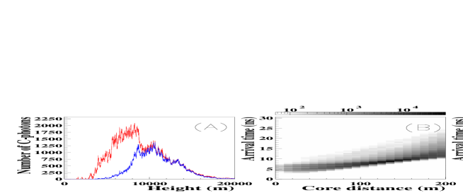
Figure 13: Time structure of a typical gamma-ray initiated shower. b. The arrival time as a function distance from the core in meters for a typical gamma shower. The shading is proportional to the Cherenkov-photon density. c. Same as b. but only those photons with an arrival direction within 0.3^∘ from the direction towards the shower maximum from a position on the ground are displayed for the same showers. a. Number of Cherenkov-photon emitting electrons in the shower as a function of height a.s.l.

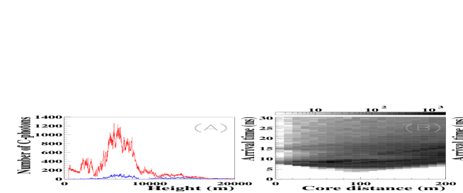
Figure 14: Time structure of a typical proton initiated shower. The panels show the same quantities as in the previous fig.13. Note that the proton emits a much smaller fraction of light within the restricted field-of-view because of its larger angular extension.

Figure 15: Sketch to illustrate the effect of a small-field of view - necessitated by the heliostat-field approach - on the determination of the timing structure. A gamma-ray induced shower is symbolized in the left part of the figure and a proton induced one with a slightly different incidence direction on the right. The proton shower is spatially more extended and symbolized as a collection of small sub showers. The restricted field of view “projects” out sub showers in the central part of the shower out of the more extended proton shower. Other more penetrating and laterally extended sub showers - that increase the fluctuation in the timing front - do not contribute to the light detected within the restricted field of view. One sub shower with an incidence direction biased towards the pointing direction (symbolized by the label “sub”) is preferentially detected and thus biases reconstructed directions towards the pointing direction.

4.5.2 Reconstructed direction of proton induced showers

Another important method to discriminate gamma- and proton induced showers is to exclude all showers that do not arrive from the source direction within the angular resolution as determined with a fit to the timing front. With a restricted field of view there is a bias of the shower direction reconstructed from timing information towards the source direction (see fig.15). The field-of-view “selects” a part of the shower which lies towards the shower maximum of a shower arriving from the source direction. The timing-fit then finds the direction of this subpart of the shower, which is biased towards the source direction. In Monte-Carlo simulations of proton induced showers we found that the mean difference between true shower direction and reconstructed shower direction is 0.71^∘ $\pm$ 0.002^∘ (statistical error), whereas the mean difference between source direction and reconstructed shower direction is only 0.44^∘ $\pm$ 0.002^∘ (statistical error). This bias decreases the fraction of proton showers which can be excluded due to their angular distance to the source direction.

4.5.3 Energy resolution

The restriction in the field of view decreases the energy resolution progressively for large showers, because the fraction of the shower image seen cannot be inferred. We find that near our energy threshold for gamma rays the resolution derived from choosing the total charge recorded in all 4 cones as simple primary-energy estimator is about 110$\%$ and worsens rapidly for higher energies.

5 Data selection

5.1 Detector condition

Only nights in which all four detector channels and the heliostats in the field were functioning normally according to the recorded monitor files were chosen for further analysis.

5.2 Meteorological selection

It was found that the reconstruction quality depends on the atmospheric transmission. For example in nights which were visibly hazy with a high relative humidity above 80$\%$ (a relatively frequent nightly weather condition at the PSA), the total trigger rate was low, the ratio of well reconstructed events to events with a misreconstructed angular direction (called “PT” below) was reduced by up to a factor 2 and the ${\rm lsq_{t}^{2}}$ of the fit to the timing front significantly increased. This is probably the result of selective absorption, by which Cherenkov light from the deeply penetrating part of the airshower, with increased temporal fluctuations, dominates the recorded signal. As $\gamma$-induced showers develop mainly in the upper atmosphere a selection of data without selective absorption is important. Besides a relative humidity below 70$\%$ and generally clear skies we required the following criteria from the reconstructed data of a given night. The parameter limits for each individual pointing direction were chosen such that a set of “good” nights —defined as showing fairly constant parameter values—was retained. The parameter limits thus slightly varied for different pointing directions.
First a cut to exclude unstable weather conditions was applied. For this the fraction of events with a reconstructed angle far from the source direction was chosen.
Condition 1: 0.95 $<$ RO $<$ 1.05
RO = (Number of events with reconstructed direction $>$ 3^∘ from pointing direction ON source) / (Number of events with reconstructed direction $>$ 3^∘ from pointing direction OFF source)
The other two run-cut criteria are meant to exclude nights with low atmospheric transmission.
Condition 2: Rate after all software cuts in OFF source direction $>$ 50/min
Condition 3: PT $>$ 0.8
PT = (Number of events with reconstructed directions $<$ 1^∘ from pointing direction OFF source)/ (Number of events with reconstructed directions $>$ 3^∘ from pointing direction OFF source)
These “meteorological cuts” are severe under the weather conditions at the PSA. In the data sample on Crab in February/March 2000 only 22$\%$ of all data taken on the Crab pulsar passed all cuts.

6 Data reduction—the problem of different conditions in the source and OFF-source region

A fundamental problem of all Cherenkov experiments—specially for those attempting to detect an excess due to gamma-rays in the total rate—is the fact that the night-sky background between ON- and OFF-source differs in general. This can influence the counting rate and analysis efficiency in various ways. This problem is most critical for the heliostat-array based experiments because they aim to work with a trigger threshold near to random fluctuations of the night-sky background in a single channel. We discuss the observed differences in the ON- and OFF-source region in section 6.1. Sections 6.2 and 6.3 discuss the effect of a difference in the ON- and OFF-source intensity of the NSB on the total rate and the reconstruction, respectively. Section 6.4 describes the method we finally chose to calculate an excess of events in the ON-source direction.

6.1 Detailed comparison of conditions ON and OFF source

For the counting conditions chosen in the 1999/2000 season, the “q-trigger” (see section 2.2.2) leads to random event triggers due to night-sky noise. Because this random rate is very sensitive to the night-sky background, slightly higher NSB levels in OFF (as observed for all potential sources see tables (2 - 5)) produce a higher event-trigger rate in OFF (see entry “raw events” in tables 2-4) The random rate was calculated from the recorded single rates. A discussion of the total rate after a correction for the random trigger and other small effects is given below in section 6.2. From test data it was shown that the reconstruction of the timing shower front always fails for random-trigger events, so that the event number “after reconstruction” (“rec. events” in tables 2 - 4) is expected to be free from night-sky background induced random triggers.
All 4 sources discussed in this paper show a slightly higher NSB in the OFF-source region. This effect is most pronounced for the source 3C 454, where—from the data reported in table 3—the current (q-rate) is 13 (25)$\%$ higher in OFF than in ON. However, the measured RMS fluctuation is only 0.4$\%$ higher in OFF than in ON and this difference is smaller for the other sources (0.04$\%$ for the Crab pulsar). By measuring the random noise in complete darkness, we determined a constant night-sky background independent noise level with a RMS of 0.8658. Subtracting this constant noise quadratically from the total noise we get the contribution from the NSB alone (number in brackets in third column of table 2 - 5). For the source with the largest difference in noise level, the NSB-induced component differs in ON- and OFF-source position by about 2.5$\%$, so that the difference in brightness at the two positions can be estimated to be about 5$\%$.
An effect that is very difficult to remove is a slight expected reduction in the trigger threshold due to a higher NSB. Due to fluctuations, smaller events can cross the trigger threshold. The opposite effect—that large events are decreased in amplitude due to fluctuations and fail to cross the threshold—happens less often due to a CR spectrum that steeply falls with amplitude.

Table 2: Current (mean of 4 Cones), q-rate: single trigger rate of charge integrating channel (mean of Cone 1+2), $\bf\sigma_{\rm NSB}$: RMS fluctuation of the measured NSB (in flash-ADC units) in the first 100 channels (before signal), number in brackets is NSB induced background alone, log(mean q): base-10 logarithm of mean net-charge (in flash-ADC units) of all events in sample, raw events: all hardware-triggered events which traces were recorded, rec. events: number of events after angular reconstruction and software trigger, centr. events: normalized number of events in central angular region (within 0.7 degrees of pointing direction), calculated as explained in section 6.4. Rows are for the samples with pointing towards the Crab pulsar (“ON”) and on a sky position (“OFF”) with a right ascension 2.625 degrees larger than in the ON direction. The total data-taking time ON was 430 minutes with an equal amount of OFF time.

	current [$\mu$A]	q-rate[kHz]	$\sigma_{\rm NSB}$ [ADC units]	log(mean q)
ON	19.0 $\pm$ 0.4	1.35	0.9493 (0.3893)	2.940 $\pm$ 0.004
OFF	19.3 $\pm$ 0.3	1.49	0.9497 (0.3902)	2.937 $\pm$ 0.004
EXCESS	-0.3	-0.14	-0.0004 (-0.0009)	0.003 $\pm$ 0.006

	raw events	rec. events	centr. events
ON	68702	33384	9415
OFF	75198	33056	8678
EXCESS	-6496 $\pm$ 379	328 $\pm$ 258	737 $\pm$ 165

Table 3: Entries as in table 2 for the samples with pointing towards the radio source 3C 454.3 (“ON”) and on a sky position (“OFF”) with a right ascension 2.625 degrees larger than in the ON direction. The total data-taking time ON was 550 minutes with an equal amount of OFF time.

	current [$\mu$A]	q-rate[kHz]	$\sigma_{\rm NSB}$ [ADC units]	log(mean q)
ON	17.7 $\pm$ 0.4	3.1	0.9505 (0.3922)	3.119 $\pm$ 0.003
OFF	20.3 $\pm$ 0.3	4.1	0.9540 (0.4006)	3.113 $\pm$ 0.003
EXCESS	-2.6	-1.0	-0.0035 (-0.0084)	0.006 $\pm$ 0.004

	raw events	rec. events	centr. events
ON	42516	30570	7525
OFF	44949	30889	7625
EXCESS	-2433 $\pm$ 296	-319 $\pm$ 248	54 $\pm$ 141

Table 4: Entries as in table 2 for the samples with pointing towards the unidentified $\gamma$-ray source 3EG J1835+59 (“ON”) and on a sky position with a right ascension 2.625 degrees larger than in the ON direction. The total data-taking time ON was 490 minutes with an equal amount of OFF time. The result for the central region is not given for this source because the quality of the angular reconstruction was strongly decreased for its direction pointing towards the north.

	current [$\mu$A]	q-rate[kHz]	$\sigma_{\rm NSB}$ [ADC units]	log(mean q)
ON	15.5 $\pm$ 0.6	1.7	0.9528 (0.3977)	3.122 $\pm$ 0.002
OFF	15.8 $\pm$ 0.6	1.8	0.9519 (0.3956)	3.116 $\pm$ 0.002
EXCESS	-0.3	-0.1	0.0009 (0.0021)	0.006 $\pm$ 0.003

	raw events	rec. events	centr. events
ON	45984	21639	-
OFF	46431	21772	-
EXCESS	-447 $\pm$ 304	-25 $\pm$ 212	-

Table 5: Entries as in table 2 for the samples with pointing towards a “pseudo source” at right ascension = 330.68 degrees and declination = 40.28 degrees (“ON”) and on a sky position with a right ascension 2.625 degrees larger than in the ON direction. The total data-taking time ON was 250 minutes with an equal amount of OFF time.

	current [$\mu$A]	q-rate[kHz]	$\sigma_{\rm NSB}$ [ADC units]	log(mean q)
ON	16.6 $\pm$ 0.5	4.3	0.9564 (0.4063)	2.991 $\pm$ 0.003
OFF	17.3 $\pm$ 0.5	5.7	0.9588 (0.4119)	2.993 $\pm$ 0.003
EXCESS	-0.7	-1.4	-0.0024 (-0.0056)	-0.002 $\pm$ 0.005

	raw events	rec. events	centr. events
ON	24119	13136	2295
OFF	26911	13272	2299
EXCESS	-2792 $\pm$ 226	-136 $\pm$ 136	-7 $\pm$ 76

This effect was studied by calculating the total mean charge of all ON versus all OFF source events ( see tables 2 - 5 entry “mean q”). If small events are preferred, the total mean charge should be smaller by a certain factor f_b with increased NSB. The total rate should be increased by a factor of roughly f${}_{b}^{1.4}$ for our setup.
It can be seen from the results in the tables (2 - 4) that within the statistical error of typically somewhat less than a percent the total mean charge is the same for all sources. However, within this error a significant reduction of the threshold - one which would produce a reduction in ON-OFF rates of the same order of magnitude as an expected signal from the crab nebula - cannot be excluded in this way.

6.2 Effect of NSB differences on total trigger rate - Monte-Carlo simulation

The effect of the NSB differences on the total trigger rate was simulated by raising the amount of random noise by 5$\%$ over its usual value. The detector Monte Carlo models the electronic pulse shaping and the response of the discriminator in detail (see fig.16), and so the effective change in threshold, due to the increased noise level could be deduced to be about 6$\pm$ 2$\%$.

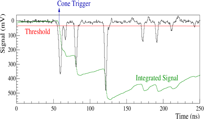
Figure 16: Trigger simulation in the detector Monte Carlo. A trace with high time resolution is integrated in the electronic chain of the “charge(q)-trigger”(section 2.2.2), resulting in the signal labelled “Integrated signal”. Once this signal surpasses the threshold level, a Cone Trigger is initiated.

Extrapolating, we deduce an expected spurious excess at the OFF source position for the source with the largest difference in ON and OFF noise (3C454, see table 3) of about 1$\%$, this corresponds to about 1.4 $\sigma_{\rm stat}$ in this case. As the difference in the noise levels between ON and OFF is smaller in the case of the other 3 sources discussed in this paper, this effect does not yet contribute significantly. However, it is clear that a very careful correction for it becomes necessary when the available statistics grows.

6.3 Effect of NSB differences on reconstruction - Software padding

Finally a difference in NSB leads to a slightly different noise levels in ON and OFF data. For example for the Crab data the RMS noise in the ON-source data was found to be about 0.5$\%$ smaller than in the OFF-source data. The effect of this difference on the reconstruction procedure was studied by artificially adding noise at the software level (“software padding”). Fig.17 demonstrates that the fraction of events near the source direction (“PT” of section 5.2) decreases with increasing NSB, but that the effect is important only at relatively large increases on the order of a few percent. From the results shown in figure 17 it was derived that an increase of RMS noise by 1$\%$ decreases the overall reconstruction efficiency by about 0.4$\%$ and the peak to tail ratio PT (section 5.2) by 0.8$\%$. This effect remains small for the observed fractional differences of the RMS NSB-noise in ON and OFF (on the order a few tenths of a percent at maximum (see table 2- 5)), and was neglected in the present analysis. It must be noted that software padding is not a perfect simulation of the real conditions, because the influence of the NSB on the hardware-trigger condition—which can in principle influence shower properties and reconstruction—is not simulated.

Figure 17: The number of showers as a function of difference in zenith angle to the source direction reconstructed with the experimental NSB (full line) and NSB increased on the software level (dashed line) by 0.06$\%$ (upper plot), 0.9$\%$ (middle plot) and 30$\%$ (lower plot). In the lower plot a decrease of the fraction of events within the central region is obvious.

6.4 Calculation of the excess

To avoid the problem mentioned in section 6.2 we chose a method that normalizes any excess to the ratio of ON- and OFF-source events for the final results reported in the next section.
The normalized excess EXCESS_n was calculated according to the following equation:

(3) $$\rm{EXCESS_{n}=ON_{in}-OFF_{in}\left(ON\over OFF\right)_{out}}$$

Here $\rm{(ON,OFF)_{in}}$ stands for the number of events within 0.7^∘ from the source and OFF-source direction, respectively whereas $\rm{(ON,OFF)_{out}}$ stands for the number of events with directions deviating more than 2^∘ from the source direction. The statistical error of EXCESS_n, ERR_n was calculated according to:

(4) $$\rm{ERR_{n}}=\left(ON_{in}+OFF_{in}\times\left(ON\over OFF\right)_{out}^{2}+\left[{(1+\left(ON\over OFF\right)_{out})ON_{out}\times OFF_{in}^{2}}\over OFF_{out}^{2}\right]\right)^{0.5}$$

7 Results

7.1 Crab pulsar

Several parameters of the data set taken on Crab pulsar are presented in table 2. A parameter n_t=5 for the software-trigger was chosen (section 3.1). Fig. 18 shows the number of events as function of angular distance from the source direction, both for ON- and OFF-source direction and the normalized difference ON-OFF. An excess of events in the angular region expected from Monte-Carlo simulations (fig.18) is seen, we find
EXCESS_n = 737 $\pm$ 165
calculated according to eqns (3,4). This corresponds to a 4.5 $\sigma$ excess and a mean excess rate EXCESS_nr = 1.7/min. Fig.20 displays the excess as a projection onto zenith and azimuth axis respectively. An integral flux $\phi_{int}$ is calculated from this excess according to:

(5) $${\rm\phi_{int}=(EXCESS_{nr}/r_{\gamma})(r_{p}/r_{\rm obs})t_{c}\phi_{whipple}}$$

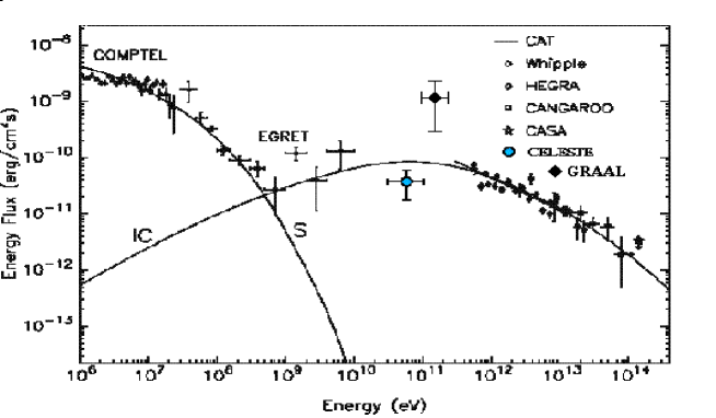
Figure 21: The energy flux as a function of energy as determined here (diamond) compared to determinations in other experiments (adapted from [12]).

Here $\phi_{\rm whipple}$= $\int_{\rm E_{\rm thresh}}^{\infty}$ 3.3 $\times$ 10^-7 E^-2.4 m^-2 sec^-1 TeV^-1 dE is the integral gamma-ray flux from the Crab above a threshold energy E_thresh as observed by the Whipple collaboration[18]. r_γ is the gamma-ray rate expected in GRAAL from the Monte-Carlo simulated effective area for gammas of fig.7 based on this flux (0.011 Hz). Note that the absolute Whipple flux cancels in eq.5, and we only adopt the spectral index from ref.[18]. r_p is the proton rate expected in GRAAL on the basis of the known proton flux $\phi_{ref}$ and the effective area for protons of fig.7 (4.0 Hz). r_obs is the observed cosmic-ray rate in the final reconstructed sample, corrected for dead time (1.6 Hz). The factor (r_obs/r_p) is an empirical correction for the fact that our Monte-Carlo calculated proton effective area fig.7 predicts a somewhat higher proton rate than observed. t_c is a correction factor for the fact that some photons are expected in the “outer angular region” and was determined as 2.2 (1.4) from weighted (unweighted) Monte Carlo data. The weighted value was chosen for the final result. The final integral flux above threshold assuming a differential spectral source index of -2.4 is:
$\phi_{int}$ = 2.2 $\pm$ 0.4 (stat) ${}^{+1.7}_{-1.3}$ (syst) $\times$ 10^-9 cm^-2 sec^-1 above threshold
The systematic error of our flux determination is dominated by the uncertainty in absolute light-calibration. The conversion factor “total light at entrance of Cone vs. flash ADC channel” used in the Monte-Carlo simulation for the effective detection area can be compared with the one derived from the LED based method described in section 2.2.4 for all four Cones. The relative difference:
((predicted ADC channel Monte Carlo) - (predicted ADC channel LED))/ (predicted ADC channel Monte Carlo)
was 21$\%$,-31$\%$,-13$\%$,+29$\%$ for Cone 1-4. From this we estimate a systematic error of 30$\%$ for this conversion. We estimate a similar error due to uncertainties in the Monte Carlo simulations between the primary and the entrance of Cones which increase the error in absolute light calibration to about 42$\%$, corresponding to a flux error of about ${}_{-60}^{+81}\%$. Another important source of overall systematic error is the systematic errors of t_c (35$\%$) in which uncertainties in the spectral weighting procedure and the detailed simulation of the trigger enter and which was added in quadrature. The final adopted systematic error is ${}_{-69}^{+88}\%$. This result is compared with other flux determinations in fig.21.

7.2 Other potential sources

Fig. 19 and table 3 present a data set—of very similar size and taken under similar conditions as the data on the Crab pulsar—on the potential gamma source 3C 454.3. n_t=7 was chosen. No significant excess can be seen. Table 4 and 5 present the analysis on the potential source 3EG J1835+59 (n_t=9) and a “pseudo” source (n_t=7), with data taken with a pointing towards a dark spot in the night sky. In both cases the results are in agreement with no gamma-ray emission from these sources. The former source lies towards the north of the heliostat field. As discussed in section 2.3 this leads to a worse reconstruction of direction and a derivation of number of “central events” does not make sense.

7.3 Excess in total rate

If the detected excess (discussed in section 7) is real, one can estimate that there should be an excess of $\approx$ 2270 events within our measuring time. On the other hand, extrapolating the Whipple flux for Crab nebula ([18]) at our energy threshold, only 355 excess events are expected.
Due to our trigger setup it can happen that fluctuations of the NSB alone trigger events. The rate of these “accidental trigger” can be calculated from the single rates (properly taking into account the trigger logic discussed in section 2.2.2) and subtracted from the total rate. For the sequence trigger the probability that cones 1 and 2 trigger at the same time accidentally has been calculated from the individual sequence trigger rates of each cone. For the charge trigger the accidental events are given by the probability of 3 cones out of 4 triggering simultaneously due to the individual q-rates at each cone. The probability of accidental events is calculated every 2 seconds, so that peaks of high intensity (e.g. due to the light of a car) can be detected. The number of accidental events rises with the individual sequence and q rates. With the new setting of season 2000/2001 (data from this season are not discussed in this paper) the individual rates have been lowered so that the total rate of real events is still the same as for season 1999/2000 but there are no more accidental events. Other corrections are related to the dead time of the setup. During each run, calibrations are done regularly to verify time and amplitude of the peaks and gain properties of the electronic chain (see section 2.2.4). The time used for the calibrations can be slightly different in ON and OFF periods. It may also happen that some time is lost due to the switching off of the PMTs (for safety reasons, if the currents increase above 35$\mu$A the PMTs switch off automatically for $\approx$ 15 seconds). These 2 factors can produce a difference in measuring time in ON and OFF periods. A correction factor is applied so that periods ON and OFF have exactly the same time of measurement.

Table 6 right column shows the results of a careful correction for these effects for the same four data samples as used for tables 2 - 5 (see section 6). In the last column all the effects have been corrected. For the case of the Crab nebula there is an excess in the OFF position of 7234 events in the hardware-triggered events. After subtraction of accidental events and corrections for dead time, the excess in the OFF position is only 443 events, which is within the statistical fluctuations. For orientation, a difference in the energy threshold of cosmic-ray protons between ON and OFF of only 5 GeV at an energy threshold of 2 TeV already produces a difference of 550 events for the same time of measurement and using the known cosmic-ray proton flux and a constant effective area of 8000 m².

Table 6: Number of hardware-triggered events (labelled “total events”), number of events with subtraction of the expected number of accidental events and a correction for the overall dead time applied(labelled “total corrected events”)

Crab	Total events	Tot. correct. evs
ON	79194	58107
OFF	86428	58550
EXCESS	-7234 $\pm$ 407	-443 $\pm$ 341

3C454	Total events	Tot. correct. evs
ON	49141	49139
OFF	51982	49521
EXCESS	-2841 $\pm$ 318	-382 $\pm$ 314

3EG+1835	Total events	Tot. correct. evs
ON	50264	53760
OFF	50914	54702
EXCESS	-650 $\pm$ 318	-942 $\pm$ 329

pseudo source	Total events	Tot. correct. evs
ON	28808	26010
OFF	31993	26549
EXCESS	-3185 $\pm$ 246	-539 $\pm$ 229

In the alternative approach of applying a software threshold ( section 6.3) accidental events are rejected due to their incorrect timing pattern. Less than 0.6$\%$ of the accidental events pass the analysis for a very similar NSB to the one of Crab sample. In our analysis, a higher NSB rejects more accidental events. As seen in the column 6 of table 2 also here there is no significant excess in the total rate. This lack of an excess in the total rate seems to cast a doubt on the reality of the signal discussed in section 7.

8 Conclusion

The results of the present paper do not yet prove that the use of an heliostat array in gamma-ray astronomy is a feasible alternative to the use of dedicated Cherenkov telescopes. The properties of experimentally detected showers—while showing statistically significant deviations from Monte-Carlo simulated proton showers—agree in some important derived parameters to within typically 10$\%$. Systematic errors were within the range expected. Both the capital costs of the experiment and the running costs of remote night-time operation in a facility used for solar-energy research during daytime are lower than of a comparable dedicated telescope.
The principle drawbacks of this approach were found to be the restricted field of view and the night-time weather conditions at the relatively low elevation of the heliostat field. The field-of view restriction was shown to lead to a very similar time structure of the shower front in proton and gamma induced showers. Moreover it biases the direction reconstruction based in timing towards to the pointing direction. Both effects together prevent an efficient separation of proton and gamma induced showers. This makes a flux determination independent of total rates difficult (though not impossible) and severely limits the sensitivity of the experiment. It was found that the fraction of time (total duty cycle) with weather and moon-light conditions sufficient for the detection of gamma radiation was about 3-4$\%$ at the PSA, about a factor 5 lower than at astronomical sites. Both drawbacks seem to be unavoidable also in the future, because an enlargement of the field of view seems impossible within a budget lower than for dedicated telescopes, and the site-selection criteria for solar-energy generation facilities (e.g. low average wind speeds) exclude astronomical sites in principle. The effect of different night-sky backgrounds in the ON- and OFF-source region on the hardware trigger threshold is still small for the relatively small event numbers discussed in this paper and the observed maximal difference of NSB intensity of 5$\%$. However, this effect becomes a principal difficulty for the determination of absolute fluxes in somewhat larger samples.

Figure 18: The upper plot (a.) shows the number of events as a function of angular distance of reconstructed direction from source direction for ON-source events (full line) and OFF-source events (dashed line). No normalization of any kind was applied to this plot. The lower plot (b.) shows the difference ON - OFF, normalized to the number of events in the outer angular region, according to eq.3 Data from the Crab pulsar taken under good meteorological conditions according to the cuts discussed in section 5.2 were used. The statistical errors of the individual bins are shown.

Figure 19: Good-weather data of the potential source 3C 454.3 plotted as in fig. 18

Figure 20: The difference of the number of events in ON source direction and OFF source direction for the Crab data sample shown in fig. 18 as a function of deviation of the zenith (upper plot a.) and azimuth angle (lower plot b.) from the source direction.

Acknowledgments The GRAAL project is supported by funds from the DFG, CICYT and the EC-DGXII’s ’Improving Human Potential programme “Access to large scale facilities”. We thank the PSA—in particular A.Valverde—for excellent working conditions at the CESA-1 heliostat field. We thank the ”Centro de Supercomputacion UCM” for support.

References

- [1] F.Krennrich, TeV Gamma-Ray Astronomy in the new Millennium, Proc. 7th Taipei Astrophysics Workshop, ASP Conference Series, Vol. XX, 2001, de. C.M. Ko,astro-ph/0101120.
- [2] D.Borque, PhD thesis, to be published, Universidad Complutense, Madrid, (2001).
- [3] M.Diaz, PhD thesis, to be published, Universität Heidelberg, (2002).
- [4] D. Dumora et al. (CELESTE coll.), Cherenkov Low Energy Sampling & Timing Experiment - CELESTE experimental proposal, http://wwwcenbg.in2p3.fr/Astroparticule (1996).
- [5] S.Danaher, D.J.Fegan, N.A.Porter, T.C. Weekes, T.Cole, Possible applications of large solar arrays in astronomy and astrophysics, Solar Physics 28 (1982) 335-343.
- [6] O.T. Tümer,T.J. O´Neill, A.D.Zych, R.S.White, A large area VHE detector with low-energy threshold, Proc. 21st ICRC, Adelaide, 4 (1990) 238-241.
- [7] O.T. Tümer, A.D. Kerrick, T.J. O´Neill, R.S.White, A.D.Zych, Solar One Gamma Ray observatory for intermediate high energies of 10 - 500 GeV, Proc. 22nd ICRC, Dublin 2 (1991) 634-637.
- [8] B.Giebels et al. (CELESTE coll.), Prototype Tests for the CELESTE Solar Array Gamma-Ray Telescope, astro-ph/9803198, Nucl.Inst.& Meth. A412 (1998) 329.
- [9] The STACEE coll., The Solar Tower Atmospheric Cherenkov Effect Experiment (STACEE) Design Report, EFI preprint 97-17 (1997).
- [10] M.C. Chantell et al.(STACEE coll.) Prototype Test Results of the Solar Tower Atmospheric Cherenkov Effect Experiment (STACEE), astro-ph/9704037, Nucl.Inst.Meth. A408 (1998) 468.
- [11] J.A.Zweerink et al., The Solar Two Gamma-Ray Observatory: Astronomy between 20 and 300 GeV, Proc. 26th ICRC 5 (1999) 223.
- [12] M. de Naurois et al. (CELESTE coll.), Status and current sensitivity of the CELESTE Experiment, astro-ph/0010265 (2000); J.Holder, Observation of Mkn 421 with the CELESTE Experiment, astro-ph/0010264 (2000).
- [13] S.Oser et al. (STACEE coll.), High Energy Gamma-Ray Observations of the Crab Nebula and Pulsar with the Solar Tower Atmospheric Cherenkov Effect Experiment, astro-ph/0006304 (2000), Ap.J. submitted.
- [14] D. Heck, J. Knapp, J.N. Capdevielle, G. Schatz, T. Thouw, CORSIKA: A Monte Carlo Code to simulate Extensive Air Showers, Forschungszentrum Karlsruhe Report FZKA 6019 (1998); find this report and further information at: http://ik1au1.fzk.de/heck/corsika/
- [15] R.Plaga, J.Fernandez, J.Gebauer, M.Haeger, A.Karle, On the possible use of the solar power plant CESA-1 field at Tabernas as Cherenkov detector, 24th ICRC (Rome) Vol.1 (1995),1005.
- [16] F.Arqueros et al., The Mini-GRAAL project, Proc. “Towards a Major Atmospheric Cherenkov Detector IV”,O.C.de Jager(ed.) (1997) 240-246.
-
[17]
B.Wiebel,
Chemical composition in high energy cosmic rays,
Report WUB 94-08 (1994), available on http://
wpos6.physik.uni-wuppertal.de:8080
/Public/papers-public.html - [18] A.M.Hillas et al.,Spectrum of TeV Gamma Rays from the Crab Nebula, Astrophys.J. 503 (1998) 744.
- [19] J.R.Patterson, A.M.Hillas, Optimizing the Design of Very High Energy Gamma-Ray Telescopes, Nucl.Inst.& Meth. A278 (1989) 553.
- [20] V. R. Chitnis, P. N. Bhat, Possible Discrimination between Gamma Rays and Hadrons using Cerenkov Photon Timing, Astropart.Phys. 15 (2001) 29-47.