Qualitative Properties of Magnetic Fields in Scalar Field Cosmology

Abstract

We study the qualitative properties of the class of spatially homogeneous Bianchi VI${}_{\mbox{o}}$ cosmological models containing a perfect fluid with a linear equation of state, a scalar field with an exponential potential and a uniform cosmic magnetic field, using dynamical systems techniques. We find that all models evolve away from an expanding massless scalar field model in which the matter and the magnetic field are negligible dynamically. We also find that for a particular range of parameter values the models evolve towards the usual power-law inflationary model (with no magnetic field) and, furthermore, we conclude that inflation is not fundamentally affected by the presence of a uniform primordial magnetic field. We investigate the physical properties of the Bianchi I magnetic field models in some detail.

I Introduction

There are many observations that imply the existence of magnetic fields in the Universe, and recent observations have produced firmer estimates of the strength of magnetic fields in interstellar and intergalactic space (Kronberg, 1994; Kronberg et al., 1992; Wolf et al., 1992). The observations to date place an upper bound on the strength of a cosmic magnetic field, but are not conclusive as to whether such a field exists (see Vallée 1990a,b). Although cosmologists have investigated the possible existence of a homogeneous intergalactic magnetic field of primordial origin both from a theoretical and an observational point of view for many years, research on cosmological magnetic fields has been rather marginal despite their potential importance. The reasons could be the perceived weakness of the field effects or the lack, as yet, of a consistent theory explaining the origin of cosmic magnetism. However, this situation has changed considerably recently (cf. Grasso and Rubenstein, 2000).

Primordial magnetic fields introduce new ingredients into the standard picture of the early Universe. Such a field would affect the temperature distribution of the microwave background radiation, primeval nucleosynthesis and galaxy formation. But its most direct observational effect is the Faraday rotation it would cause in linearly polarized radiation from observed extragalatic radio sources. Fundamental properties of magnetic fields include their vectorial nature, which inevitably couples the field to the spacetime geometry, and the resulting tension (i.e., the negative pressure) exerted along the field’s lines of force (Parker, 1979; Matravers and Tsagas, 2000 ). The implications of such an interaction are both kinematical and dynamical; kinematically, the magneto-curvature effect tends to accelerate positively curved perturbed regions, while it decelerates regions with negative local curvature and, dynamically, the most important magneto-curvature effect is that it can reverse the pure magnetic effect on density perturbations (Tsagas and Barrow, 1997 and 1998; Tsagas and Maartens, 2000 and 2001).

In a recent analysis (Matravers and Tsagas, 2000) the kinematics were considered and, assuming a spacetime filled with a perfectly conducting barotropic fluid permeated by a weak primordial magnetic field while treating the energy density and the anisotropic pressure of the field as first-order perturbations upon the Friedmann-Lemaître-Robertson-Walker (FLRW) background, it was shown how a cosmological magnetic field can modify the expansion rate of an almost-FLRW universe. The effects of the interaction between magnetism and geometry in cosmology are subtle, and it was argued that the magneto-curvature coupling could make the field into a key player irrespective of the magnetic strength. Indeed, even weak magnetic fields can lead to appreciable effects, provided that there is a strong curvature contribution. This was illustrated by studying spatially open cosmological models containing ‘matter’ with negative pressure, and it was found that the phase of accelerated expansion, which otherwise would have been inevitable, may not even happen. This leads to the question of the efficiency of inflationary models in the presence of primordial magnetism. Recall that an initial curvature era was never considered as a problem for inflation, given the smoothing power of the accelerated expansion. However, this may not be the case when a magnetic field is present, no matter how weak the latter is. In more recent work Tsagas (2000) has further studied the vector nature of magnetic fields and discussed the unique coupling between magnetism and spacetime curvature in general relativity which gives rise to a variety of effects with important implications.

Observations of the high degree of isotropy of the cosmic microwave background indicate that the Universe is ‘almost’ isotropic and spatially homogeneous (at least since the time of last scattering). Theoretical support for this belief comes from the so-called Ehlers-Geren-Sachs (1964) Theorem. Clarkson and Coley (2001) have proven a generalization of this theorem and have consequently shown that any strong magnetic fields in the Universe are ruled out. This theoretical result is model-independent and includes the case of inhomogeneous magnetic fields. In further work (Clarkson et al., 2001) numerical constraints are placed on all types of primordial and protogalactic magnetic fields in the Universe from cosmic microwave background data.

We shall study open spatially homogeneous cosmological models containing both a uniform magnetic field and a scalar field here, partially in an attempt to address some of the questions raised above. Scalar field cosmological models are of great importance in the study of the early Universe. Models with a variety of self-interaction potentials have been studied, and one potential that is commonly investigated and which arises in a number of physical situations has an exponential dependence on the scalar field (Wetterich, 1988; Ferreira and Joyce, 1997). There have been a number of studies of spatially homogeneous scalar field cosmological models with an exponential potential, with particular emphasis on the possible existence of inflation in such models (Halliwell, 1987; Kitada and Maeda, 1993; and Billyard et al., 1999, and references within).

Dynamical systems methods for analysing the qualitative properties of cosmological models have proven very useful (Wainwright and Ellis, 1997; Coley, 1999). A qualitative analysis of cosmological models with matter and a uniform magnetic field has been presented previously (Collins, 1972; LeBlanc et al., 1995). A universe with a primordial magnetic field is necessarily anisotropic. Thus, in order to investigate the influence of the magnetic field on the dynamics of the universe the Einstein field equations must be analysed in models more general than the FLRW models. The simple classes of the Bianchi I and Kantowski-Sachs models were discussed (cf. Jacobs, 1969), and Collins (1972) applied techniques from the theory of planar dynamical systems to prove qualitative results about the evolution of the class of axisymmetric Bianchi I cosmologies with matter and a primordial magnetic field.

In LeBlanc et al. (1995) the Einstein-Maxwell field equations for orthogonal Bianchi VI${}_{\mbox{o}}$ cosmologies with a $\gamma$-law perfect fluid and a pure, homogeneous source-free magnetic field were written as an autonomous differential equation in terms of expansion-normalized variables. It was shown that the physical region of state space is compact, and that the differential equation admits certain invariant sets and monotone functions which play an important role in the analysis. A complete analysis of the stability properties of the equilibrium points of the differential equation and a description of the bifurcations that occur as the equation of state parameter $\gamma$ varies was given . The associated dynamical system was studied and the past, intermediate and future evolution of these models was determined. All asymptotic states of the models, and the likelihood that they will occur, were described. In particular, oscillatory behaviour also occurs in cosmological models with a magnetic field (and in Einstein-Yang-Mills theory in general). Further work on spatially homogeneous models with a magnetic field and a non-tilted perfect fluid has been carried out recently (LeBlanc, 1997 and 1998). In particular, Weaver (2000) has generalized (to the non-polarized solutions) the work of Leblanc et al. (1995), and rigorously shown that the evolution toward the singularity is oscillatory in Bianchi VI₀ vacuum models.

The reasons for concentrating on the Bianchi VI${}_{\mbox{o}}$ models are ones primarily of mathematical simplicity. It is well known (Hughston and Jacobs 1970) that a pure magnetic field is only possible in Bianchi cosmologies of types I, II, VI${}_{\mbox{o}}$, VII${}_{\mbox{o}}$ (in class A) and type III (in class B). For types VI${}_{\mbox{o}}$ and VII${}_{\mbox{o}}$, the algebraic constraints that arise from the Einstein field equations imply that the shear eigenframe is Fermi-propagated, which in turn implies that the remaining field equations reduce to an autonomous differential equation with a polynomial vector field. Finally, for type VI${}_{\mbox{o}}$ but not for VII${}_{\mbox{o}}$, the physical region of state space is compact. We note that since a magnetic field is not compatible with Bianchi types VIII and IX (for example), the class of Bianchi VI${}_{\mbox{o}}$ magnetic cosmologies is of the same generality as the Bianchi VIII/IX models (without magnetic field) (Wainwright 2000).

In this paper we shall investigate the class of Bianchi VI${}_{\mbox{o}}$ models with barotropic matter, a scalar field with an exponential potential and a uniform magnetic field. We shall discuss some general properties of the complete class of models, and then investigate the special case of the Bianchi I system in detail. We note that this is not the general class of Bianchi I cosmological models; we are only considering those Bianchi I models that occur as subcases of the Bianchi VI${}_{\mbox{o}}$ models with one magnetic degree of freedom. It is also of interest to study the Bianchi II cosmologies, since although they are very special within the full Bianchi class, they play a central role since the Bianchi II state space is part of the boundary of the state space for all higher Bianchi types (i.e., all types except for I and V). The Bianchi II models will be investigated in detail elsewhere (Quinlan, 2002).

The Bianchi I system in the absence of a scalar field was first qualitatively analysed in (Collins, 1972). A qualitative analysis of the Bianchi I models in the absence of a magnetic field was given in (Billyard et al., 1999); in this work the well-known power-law inflationary solution (Wetterich, 1988; Kitada and Maeda, 1993) was shown to be a stable attractor for an appropriate parameter range in the presence of a barotropic fluid in all Bianchi class B models (previous analysis had shown that this power-law inflationary solution is a global attractor in spatially homogeneous models in the absence of a perfect fluid, except for a subclass of Bianchi type IX models which recollapse). One of the aims of the present analysis is to study the stability of this model with respect to magnetic field perturbations.

II The Bianchi VI${}_{\mbox{o}}$ Models

We shall follow the approach of LeBlanc et al. (1995) in which the theory of dynamical systems was used to give a detailed analysis of the evolution of orthogonal Bianchi cosmologies of type VI${}_{\mbox{o}}$ with a perfect fluid and a magnetic field as source. This work extended that of Wainwright and Hsu (1989) who had studied perfect fluid Bianchi cosmologies of class A using state variables that are dimensionless and have a direct physical or geometric interpretation in terms of the shear of the cosmological fluid, the spatial curvature and the magnetic field, leading to a state space that is a compact subset of ${\mathbb{R}}^{5}$, which implies that a unified treatment of the asymptotic behaviour of the models at early and late times can be given. We note that all of the equilibrium points of the differential equation correspond to self-similar exact solutions of the Einstein field equations.

An invariant orthonormal frame of vector fields on the spacetime are introduced in which one vector is aligned along the fluid flow vector so that the remaining three spatial vectors (triad) span the tangent space orthogonal to the fluid flow at each point of the group orbits. The commutation functions of this frame are then taken as the basic variables. The Einstein-Maxwell field equations for a pure magnetic field are then derived in the orthonormal frame formalism, giving rise to a set of evolution equations for the shear variables ($\sigma_{\alpha\beta}$), the curvature variables ($n_{\alpha\beta}$), the energy density (conservation equation), the magnetic field (Maxwell equation) and a first integral (the Friedmann constraint), where the remaining freedom in the choice of spatial tetrad was used to simultaneously diagonalize $\sigma_{\alpha\beta}$ and $n_{\alpha\beta}$.

Expansion-normalized variables are then introduced, leading to a reduced set of evolution equations (the dynamical system) for the dimensionless shear variables $\Sigma_{\pm}$, the spatial curvature variables $N_{\alpha}$, the dimensionless magnetic field variables and the density parameter (defined as usual). Defining a dimensionless time variable, the reduced evolution equations in the special case of a Bianchi VI${}_{\mbox{o}}$ were then established (in this case there is a single dimensionless magnetic field variable, $M$).

A The Equations

We assume a scalar field with an exponential potential $V=V_{0}e^{k\phi}$, where $V_{0}$ and $k$ are positive constants, and a separately conserved perfect which satisfies the barotropic equation of state $p=(\gamma-1)\rho$, where the constant $\gamma$ satisfies $0\leq\gamma\leq 2$ (although we shall only be interested in the range $0<\gamma<2$ here). The energy conservation and Klein-Gordon equations become:

$$\dot{\rho} = -3\gamma H\rho,$$ (1)

$$\ddot{\phi} = -3H\dot{\phi}-kV,$$ (2)

where $H$ is the Hubble parameter, an overdot denotes ordinary differentiation with respect to time $t$, and units have been chosen so that $8\pi G=1$.

We also assume a uniform magnetic field (in the ‘$x$’ direction) which satisfies the Maxwell equations. The form of this magnetic field, which we shall denote here as $M^{2}$, is given in Collins (1972) or LeBlanc et al. (1995), but its precise form is unimportant since we use the generalized Friedmann constraint to eliminate $M^{2}$ from the evolution equations.

We define

$$\Omega\equiv\frac{\rho}{3H^{2}},~{}~{}~{}\Phi\equiv\frac{\dot{\phi}}{\sqrt{6}H},~{}~{}~{}\Psi\equiv\frac{V}{3H^{2}},$$ (3)

two normalized (dimensionless) shear variables $\Sigma_{+}$ and $\Sigma_{-}$ (appropriately combinations of the derivatives of the metric functions divided by the Hubble parameter; Wainwright and Ellis, 1997)), and the new logarithmic time variable $\tau$ by

$$\frac{d\tau}{dt}\equiv H.$$ (4)

The evolution equations for the quantities

$$X=\left(\Sigma_{+},\Sigma_{-},\Phi,\Psi,\Omega,N_{+},N_{-}\right)\in{\mathbb{R}}^{7},$$ (5)

are then as follows:

$$\Sigma_{+}^{\prime} = (q-2)\Sigma_{+}+2(1-N^{2}_{1}-\Phi^{2}-\Psi-\Sigma_{+}^{2}-\Sigma_{-}^{2}-\Omega)-2N_{-}^{2},$$ (6)

$$\Sigma_{-}^{\prime} = (q-2)\Sigma_{-}-2N_{+}N_{-},$$ (7)

$$\Phi^{\prime} = (q-2)\Phi-\frac{\sqrt{6}k}{2}\Psi,$$ (8)

$$\Psi^{\prime} = (2q+2+\sqrt{6}k\Phi)\Psi,$$ (9)

$$\Omega^{\prime} = (2q-3\gamma+2)\Omega,$$ (10)

$$N_{+}^{\prime} = (q+2\Sigma_{+})N_{+}+6\Sigma_{-}N_{-},$$ (11)

$$N_{-}^{\prime} = (q+2\Sigma_{+})N_{-}+2\Sigma_{-}N_{+}.$$ (12)

where a prime denotes differentiation with respect to the time $\tau$ and the deceleration parameter $q$ is defined by $q\equiv-(1+H^{\prime}/H)$, where

$$q=1-N_{-}^{2}+\Sigma_{+}^{2}+\Sigma_{-}^{2}+\frac{1}{2}(3\gamma-4)\Omega+\Phi^{2}-2\Psi.$$ (13)

The physical state space is restricted to $\Omega\geq 0$ and $N^{2}_{+}\leq 3N^{2}_{-}$ (where we include equality to include models of Bianchi types I and II; LeBlanc et al., 1995). Since $N_{-}=0$ implies $N^{\prime}_{-}=0$, the subsets $N_{-}>0$ and $N_{-}<0$ are invariant. Due to a discrete symmetry in evolution equations we can, without loss of generality, restrict attention to the subset $N_{-}\leq 0$.

The magnetic field, defined through the first integral, is given by

$$\frac{3}{2}M^{2}=1-N_{-}^{2}-\Phi^{2}-\Psi-\Sigma_{+}^{2}-\Sigma_{-}^{2}-\Omega,$$ (14)

and since $M^{2}\geq 0$, all of the variables are bounded:

$$0\leq\left\{\Sigma_{+}^{2},\Sigma_{-}^{2},\Phi^{2},\Psi,\Omega,N_{+}^{2}/3,-N_{-}\right\}\leq 1.$$ (15)

Without loss of generality, we can restrict attention to the subset $M\geq 0$. There is also an auxiliary equation for the magnetic field:

$$M^{\prime}=(q-1-2\Sigma_{+})M.$$ (16)

B Discussion

A number of invariant sets of the physical state space can be identified (cf., LeBlanc et al., 1995, and Billyard et al., 1999). In addition, there are a number of monotonic functions that exist in various invariant sets (particularly on the boundary; cf. p.521 LeBlanc et al., 1995). However, we shall not present them here. Indeed, there are many (over fifty) equilibrium points, the vast majority of which are saddles, and hence in this section we shall simply comment on some of the more physically interesting local properties of the models. In the next section we shall investigate the Bianchi I models more rigorously, and a monotonic function in this invariant set will be given explicitly, in order to discuss some aspects of the intermediate or transient behaviour of the models.

1. The equilibrium point ${\cal P}:(\Sigma_{+},\Sigma_{-},\Phi,\Psi,\Omega,N_{+},N_{-})=(0,0,\frac{-k}{\sqrt{6}},1-\frac{k^{2}}{6},0,0,0),~{}M=0$ corresponds to the power-law inflationary zero-curvature (flat) FLRW model. The eigenvalues of ${\cal P}$ are $\{k^{2}-4,k^{2}-3\gamma,\frac{1}{2}(k^{2}-2)(\times 2),\frac{1}{2}(k^{2}-6)(\times 3)\}$. ${\cal P}$ exists for $k^{2}\leq 6$ and is a sink for $k^{2}<4$ and $k^{2}<3\gamma$, and is inflationary $(q<0)$ for $k^{2}<2$. In fact it is the global attractor for this range of parameter values; this result generalizes previous work by including a cosmic magnetic field (cf. Billyard et al., 1999).

2. We are particularly interested in whether there are any sinks (or sources) with $M\neq 0$ in the Bianchi VI${}_{\mbox{o}}$ state space. We know from LeBlanc et al. (1995) that there are no attractors in the absence of a scalar field, so hence we must have $M\neq 0$, $\Phi^{2}\neq 0$ (and $\Psi\neq 0$, since this leads to $M=0$). From equation (2.10) we see that $\Omega$ approaches zero at late times, so we also take $\Omega=0$ (and $q<2$). From equations (2.8), (2.9) and (2.16) we have that (for $M\neq 0$)

   $$\Phi=\frac{-4}{\sqrt{6}k}(1+\Sigma_{+}),~{}~{}~{}\Psi=\frac{4}{3k^{2}}(1+\Sigma_{+})(1-2\Sigma_{+});\quad q=1+2\Sigma_{+}.$$ (17)

   We are particularly interested in the inflationary case in which $q<0$; i.e., $-1<\Sigma_{+}<-\frac{1}{2}$. If $N_{-},N_{+}\enskip(\Sigma_{-})$ are not zero, equations (2.11) and (2.12) yield $N_{+}=\pm\sqrt{3}N_{-}$, $\Sigma_{-}=\mp\frac{1}{2\sqrt{3}}(1+4\Sigma_{+})$, whence equation (2.7) then yields $N^{2}_{-}=\frac{1}{12}(1-2\Sigma_{+})(1+4\Sigma_{+})$, which is negative for the range of $\Sigma_{+}$ under consideration! (There do exist equilibrium points with $N_{-}\neq 0,N_{+}\neq 0$ and $\Sigma_{-}\neq 0$, but these all have $q\geq 0$ (i.e., are non-inflationary) and are saddles.) Hence we consider $N_{-}=N_{+}=\Sigma_{-}=0$. Equations (2.6) and (2.13) then yield (since $\Sigma_{+}\neq\frac{1}{2}$), $\Sigma_{+}=-1+3k^{2}/(8+k^{2})$. This equilibrium point, denoted ${\cal V}$ in section V, is physical and in the state space when $4<k^{2}<8$ and is always a saddle $(N^{2}_{+}$ is increasing as orbits evolve away from ${\cal V}$ to the future). However, since $q<0$ only for $k^{2}<\frac{8}{5}~{}(\Sigma_{+}<-\frac{1}{2})$, this point is never inflationary.

We conclude that inflation is not fundamentally affected by the presence of primordial magnetism in the models under study here.

1. In LeBlanc et al. (1995) it was shown that in the absence of a scalar field that for $\Omega>0$, $1<\gamma<2$ the global sink is the equilibrium point $PM$(VI${}_{\mbox{o}}$) so that at late times all such magnetic Bianchi VI${}_{\mbox{o}}$ cosmologies are approximated by the dynamics of a self-similar Dunn-Tupper (1980) magneto-vacuum Bianchi VI${}_{\mbox{o}}$ model. This equilibrium point has an analogue here with $\Phi=\Psi=0$, but is now a saddle. Indeed, it can be easily shown that none of the equilibrium points with vanishing scalar field can be sinks. In particular, the sink in the case $\gamma=1$ in LeBlanc et al. (1995) (subset of ${\cal L}M$(VI${}_{\mbox{o}}$)) becomes a saddle.

2. All equilibrium points corresponding to models with a non-zero matter fluid, including those corresponding to the flat FLRW perfect fluid solution (Einstein de Sitter) and the flat FLRW scaling solution, are saddles.

In the above we have made some passing comments concerning the intermediate behaviour of the models, but we have not discussed this in detail. In the next section we will discuss the intermediate behaviour of the (subset) of Bianchi I models. The transient behaviour is important for assessing the physical significance of the models. For example, LeBlanc et al. (1995) also considered whether any of the Bianchi VI${}_{\mbox{o}}$ magnetic cosmologies are compatible with observations of a highly isotropic universe. For a subset of the Bianchi VI${}_{\mbox{o}}$ cosmologies, the orbits will initially be attracted to the equilibrium point ${\cal F}$ corresponding to the flat FLRW model, but will eventually be repelled by it. For such a model there will be an epoch during which the model is close to isotropy and hence will be compatible with observations. This is the phenomenon of intermediate isotropization. It will not occur for a randomly selected magnetic Bianchi VI${}_{\mbox{o}}$ model, but there will be a finite probability that an arbitrarily selected model will undergo intermediate isotropization (the probability will depend on the desired closeness to isotropy and the length of the epoch of isotropization).

1. There is an equilibrium set ${\cal K}$: $(\Sigma_{+},\Sigma_{-},\Phi,0,0,0,0)$ where $1-\Sigma^{2}_{+}-\Sigma^{2}_{-}-\Phi^{2}=0$ (and $M=0,q=2$). (These points reduce to the equilibrium set ${\cal K}_{M}$ in the absence of a magnetic field consisting of Jacobs type I solutions with no matter and a massless scalar field - Billyard et al., 1995). The eigenvalues are $\{0,0,2(1-2\Sigma_{+}),3(2-\gamma),2(1+\Sigma_{+}\pm\sqrt{3}\Sigma_{-}),6(1+\frac{k\Phi}{\sqrt{6}})\}$. There are two zero eigenvalues (corresponding to the fact that ${\cal K}$ is a $2$-parameter family of equilibrium points). An analysis shows that there is always a subset of ${\cal K}$ that acts as sources (these are, in fact, global sources); all others are saddles.

This contrasts with the situation in the absence of a scalar field in which LeBlanc et al. (1995) showed that there are no equilibrium points that are sources and argue that generically an orbit with $\Omega>0$ will pass through a transient stage and then approach the Kasner circle into the past (consisting of Kasner, Bianchi type I vacuum models). Since these equilibrium points are saddles, the orbit subsequently leaves along a uniquely determined heteroclinic orbit and then approaches the Kasner circle again. This process then continues indefinitely, and the orbit follows an infinite heteroclinic sequence of Rosen orbits and Taub orbits joining Kasner equilibrium points undergoing Mixmaster-like chaotic oscillations (the past attractor here consists of the union of the Kasner circle and a family of Rosen magneto-vacuum type I orbits and Taub vacuum type II orbits – see also Weaver, 2000).

III Bianchi I models

The evolution equations for the Bianchi I models are obtained by restricting the above equations to the zero-curvature case (i.e., $N_{\pm}=0$), whence we obtain

$$X=\left(\Sigma_{+},\Sigma_{-},\Phi,\Psi,\Omega\right)\in{\mathbb{R}}^{5},$$ (18)

and the evolution equations are as follows:

$$\Sigma_{+}^{\prime} = (q-2)\Sigma_{+}+2(1-\Phi^{2}-\Psi-\Sigma_{+}^{2}-\Sigma_{-}^{2}-\Omega),$$ (19)

$$\Sigma_{-}^{\prime} = (q-2)\Sigma_{-},$$ (20)

$$\Phi^{\prime} = (q-2)\Phi-\frac{\sqrt{6}k}{2}\Psi,$$ (21)

$$\Psi^{\prime} = (2q+2+\sqrt{6}k\Phi)\Psi,$$ (22)

$$\Omega^{\prime} = (2q-3\gamma+2)\Omega,$$ (23)

where a prime denotes differentiation with respect to the time $\tau$ and the deceleration parameter $q$ is now given by

$$q=1+\Sigma_{+}^{2}+\Sigma_{-}^{2}+\frac{1}{2}(3\gamma-4)\Omega+\Phi^{2}-2\Psi.$$ (24)

The magnetic field satisfies

$$\frac{3}{2}M^{2}=1-\Phi^{2}-\Psi-\Sigma_{+}^{2}-\Sigma_{-}^{2}-\Omega,$$ (25)

and since $M^{2}\geq 0$, all of the variables are bounded: $0\leq\left\{\Sigma_{+}^{2},\Sigma_{-}^{2},\Phi^{2},\Psi,\Omega\right\}\leq 1$.

The equations (3.1)-(3.6) can also be easily derived from the metric directly in coordinate form – see the Appendix.

A Invariant sets and Monotonic functions

The existence of monotonic functions rule out periodic and recurrent orbits in the phase space and enables global results to be obtained. When $\Omega\neq 0$, we can define $Z\equiv\Omega\Sigma_{-}^{-2}$, whence from the evolution equations above we find that

$$Z^{\prime}=3(2-\gamma)Z,$$ (26)

so that $Z$ is a monotonically increasing function for $\gamma<2$ (LeBlanc et al., 1995). From the monotonicity principle (Wainwright and Ellis, 1997) we can deduce that $\Omega\rightarrow 0$ at early times and $\Sigma_{-}^{2}\rightarrow 0$ at late times.

When $\Omega=0$, we note that

$$q-2=3\left(M^{2}+\Sigma_{+}^{2}+\Sigma_{-}^{2}+\Phi^{2}-1\right)\leq 0,$$ (27)

and so from equation (3.3) the variable $\Sigma_{-}$ is itself a monotonic function.

There are a number of invariant sets. $M=0$ is an invariant set corresponding to the absence of a magnetic field. The dynamics in this invariant set was studied in Billyard et al. (1999). $\Phi=\Psi=0$ is an invariant set corresponding to the absence of a scalar field. The dynamics in this invariant set was studied in Collins (1972). $\Omega=0$ is an invariant set corresponding to the absence of barotropic matter. This invariant set is important for studying the the early time asymptotic behaviour. Finally, $\Sigma_{-}=0$ is an invariant set which is important in the study of late time asymptotic behaviour.

B Stability of Equilibria

Let us present all of the equilibrium points and their associated eigenvalues. We shall assume here that $1\leq\gamma<2$. The case of the bifurcation value $\gamma=2$ will be discussed in Quinlan (2002). All equilibrium points correspond to self-similar cosmological models.

Equilibrium Points: $\{\Sigma_{+},\Sigma_{-},\Phi,\Psi,\Omega\}$:

1 Zero magnetic field

1. ${\cal P}$ - Power-law inflation (flat FLRW):

   $$\left\{0,0,-{\frac{k}{\sqrt{6}}},1-{\frac{k^{2}}{6}},0\right\},~{}~{}M=0,~{}~{}q={\textstyle\frac{1}{2}}k^{2}-1.$$

   
   

   Eigenvalues: $\left[k^{2}-4,k^{2}-3\gamma,{\textstyle\frac{1}{2}}k^{2}-3,{\textstyle\frac{1}{2}}k^{2}-3,{\textstyle\frac{1}{2}}k^{2}-3\right]$
   Exists provided $k^{2}\leq 6$. Sink if $k^{2}<4$ and $k^{2}<3\gamma$; saddle otherwise. Inflationary if $k^{2}<2$ (note that this is the only equilibrium point that can be inflationary).

2. ${\cal F}_{S}$ - Matter-scaling (flat FLRW; Copeland et al., 1998):

   $$\left\{0,0,-{\frac{\sqrt{6}}{2}}{\frac{\gamma}{k}},{\frac{3}{2}}{\frac{\gamma}{k^{2}}}\left(2-\gamma\right),{\frac{k^{2}-3\gamma}{k^{2}}}\right\},~{}~{}M=0,~{}~{}q={\textstyle\frac{3}{2}}\gamma-1>0.$$

   
   

   Eigenvalues: $\left[{\textstyle\frac{3}{2}}(\gamma-2),{\textstyle\frac{3}{2}}(\gamma-2),3\gamma-4,{\textstyle\frac{3}{4}}\left(\gamma-2\right)\pm{\frac{3}{4k}}\sqrt{\left(2-\gamma\right)\left(24\gamma^{2}+k^{2}\left[2-9\gamma\right]\right)}\right]$
   Exists provided $k^{2}>3\gamma$. Sink if $\gamma<{\textstyle\frac{4}{3}}$; saddle otherwise.

3. ${\cal F}$ - Einstein-de-Sitter (flat FLRW):

   $$\{0,0,0,0,1\}~{}~{}M=0,~{}~{}q={\textstyle\frac{3}{2}}\gamma-1>0.$$

   
   

   Eigenvalues: $\left[{\textstyle\frac{3}{2}}\left(\gamma-2\right),{\textstyle\frac{3}{2}}\left(\gamma-2\right),{\textstyle\frac{3}{2}}\left(\gamma-2\right),3\gamma,3\gamma-4\right]$
   Saddle.

4. ${\cal K}$ - Kasner vacuum/massless scalar field:

   $$\left\{\Sigma_{+}^{2}+\Sigma_{-}^{2}+\Phi^{2}=1,~{}\Psi=\Omega=0\right\},~{}~{}M=0,~{}~{}q=2.$$

   
   

   Eigenvalues: $\left[0,0,3(2-\gamma),2-4\Sigma_{+},6+\sqrt{6}k\Phi\right]$
   This is a 2-parameter family of equilibrium points. Sources when $\Sigma_{+}<{\frac{1}{2}}$; saddles otherwise.

2 Non-zero magnetic field

These all correspond to anisotropic models $(\Sigma^{2}_{+}+\Sigma^{2}_{-}\neq 0)$.

1. ${\cal J}$ - Matter and no scalar field (Jacobs magnetic field model; Jacobs, 1969):

   $$\left\{{\textstyle\frac{1}{4}}(3\gamma-4),0,0,0,{\textstyle\frac{3}{2}}\left(1-{\textstyle\frac{1}{4}}\gamma\right)\right\},~{}~{}M^{2}={\textstyle\frac{1}{8}}\left(2-\gamma\right)\left(3\gamma-4\right),~{}~{}q={\textstyle\frac{3}{2}}\gamma-1>0.$$

   Eigenvalues: $\left[{\textstyle\frac{3}{2}}\left(\gamma-2\right),{\textstyle\frac{3}{2}}\left(\gamma-2\right),3\gamma,{\textstyle\frac{3}{4}}\left\{\left(\gamma-2\right)\pm\sqrt{\left(2-\gamma\right)\left(3\gamma^{2}-17\gamma+18\right)}\right\}\right]$
   Exists provided $\gamma>{\textstyle\frac{4}{3}}$ (same as ${\cal F}$ for $\gamma={\textstyle\frac{4}{3}}$). Saddle.

2. ${\cal S}$ - Matter and scalar field:

   $$\left\{{\textstyle\frac{1}{4}}(3\gamma-4),0,-{\frac{\sqrt{6}}{2}}{\frac{\gamma}{k}},{\frac{3}{2}}{\frac{\gamma}{k^{2}}}\left(2-\gamma\right),{\frac{3}{8k^{2}}}\left(4k^{2}-k^{2}\gamma-8\gamma\right)\right\},~{}~{}M^{2}={\textstyle\frac{1}{8}}\left(2-\gamma\right)\left(3\gamma-4\right),~{}~{}q={\textstyle\frac{3}{2}}\gamma-1>0.$$

   Eigenvalues: $\left[{\frac{3}{2}}(\gamma-2),{\frac{3}{8}}\left\{2\left(\gamma-2\right)\pm{\frac{1}{k}}\sqrt{2\left(2-\gamma\right)\left(a\pm b\right)}\right\}\right]$

   where $a=24\gamma^{2}+3\gamma^{2}k^{2}-26k^{2}\gamma+20k^{2}$, and $b=\sqrt{\left(18k^{2}\gamma-4k^{2}+a-32k\gamma\right)\left(18k^{2}\gamma-4k^{2}+a+32k\gamma\right)}.$

   Exists provided $\gamma>{\textstyle\frac{4}{3}}$ (same as ${\cal F_{S}}$ for $\gamma={\textstyle\frac{4}{3}}$) and $\gamma\leq{\frac{4k^{2}}{k^{2}+8}}$. Sink.

3. ${\cal V}$ - Scalar field and no matter:

   $$\left\{2{\frac{k^{2}-4}{k^{2}+8}},0,-{\frac{2\sqrt{6}k}{k^{2}+8}},12{\frac{8-k^{2}}{\left(k^{2}+8\right)^{2}}},0\right\},~{}M^{2}=2{\frac{\left(k^{2}-4\right)\left(8-k^{2}\right)}{\left(k^{2}+8\right)}},~{}~{}q={\frac{5k^{2}-8}{k^{2}+8}}>0.$$

   Eigenvalues: $\left[3{\frac{k^{2}-8}{k^{2}+8}},3{\frac{k^{2}-8}{k^{2}+8}},3{\frac{4k^{2}-k^{2}\gamma-8\gamma}{k^{2}+8}},{\frac{3}{2}}\left\{{\frac{k^{2}-8}{k^{2}+8}}\pm\sqrt{{\frac{17k^{2}-72}{k^{2}-8}}}\right\}\right].$

   Exists provided $4\leq k^{2}\leq 8$. Sink when $\gamma>{\frac{4k^{2}}{k^{2}+8}}$; saddle otherwise.

C Discussion

In Table I we summarize the equilibrium points and their stability for different values of the parameters $(\gamma,k^{2})$. In Figure 1 we show the sinks in $(\gamma,k^{2})$-parameter space. The equilibrium point ${\cal P}$ represents the power-law FLRW solution with no matter and no magnetic field, and is inflationary for $k^{2}<2$. It is a global attractor for $k^{2}<3\gamma$ in the Bianchi I invariant set. Note that ${\cal P}$ is a sink in the full class of Bianchi VI${}_{\mbox{o}}$ models, unlike all other sinks in Figure 1 which are only attractors in the Bianchi I invariant set. Also note that the monotonic function $Z$ in the Bianchi I invariant set indicates that $\Omega\rightarrow 0$ at early times (at the sources) and $\Sigma_{-}\rightarrow 0$ at late times (at the sinks), consistent with the results in Table I.

The equilibrium points ${\cal S}$ and ${\cal V}$, in which all of the matter fields are non vanishing and in which matter field (only) vanishes, respectively, correspond to new exact self-similar magnetic field cosmological models. The new solutions are given explicitly in the Appendix.

Heteroclinic sequences (and hence the transient behaviour of the Bianchi I models) can easily be deduced from the Table. As a particular example, for $\gamma=5/3$ and $5<k^{2}<40/7$, a subset of $\cal K$ constitute sources (the remainder are saddles), $\cal V$ is a sink, $\cal J$ is a saddle (that lies in the $\Phi=0,\Psi=0$ ($M=0$) submanifold) and $\cal F$, $\cal P$ and ${\cal F}_{S}$ are saddles (that lie in the isotropic $\Sigma_{+}=0$, $\enskip\Sigma_{-}=0$ ($M=0$) submanifold–in this submanifold $\cal K$ is a source, $\cal F$ and $\cal P$ are saddles, and ${\cal F}_{S}$ is a sink). The heteroclinic sequence in this case is presented in Figure 2.

From the the Table and Figures we can deduce both the asymptotic and the intermediate behaviour of the Bianchi I models. Note that as $\gamma$ increases, the magnetic field becomes increasingly important at late times, consistent with the observation of Wainwright (2000) (in the absence of a scalar field).

(a)  $1\leq\gamma\leq\frac{4}{3}$ $k^{2}$ $3\gamma$ $4$ $6$ $8$ ${\cal P}$ XSINK SADDLE        does not exist ${\cal F_{S}}$ does not exist XSINK ${\cal F}$ XSADDLE ${\cal V}$ does not exist XSADDLE does not exist
(b)  $\frac{4}{3}<\gamma<2$ $k^{2}$ 4 $3\gamma$ 6 $8\gamma/(4-\gamma)$ $8$ ${\cal P}$ XSINK SADDLE does not exist ${\cal F_{S}}$ does not exist XSADDLE ${\cal F}$ XSADDLE ${\cal J}$ XSADDLE ${\cal S}$ Xdoes not exist SINK ${\cal V}$ does not exist     XSINK XSADDLE does not exist

TABLE I.: Summary of all of the equilibrium points (as defined in the text) and their nature for different $\{\gamma,k^{2}\}$-parameter values in the Bianchi I models with (a) $1\leq\gamma\leq\frac{4}{3}$ and (b) $\gamma>\frac{4}{3}$. Note that for $\frac{4}{3}<\gamma<2$,  $4<3\gamma<8\gamma(4-\gamma)^{-1}<8$, and in (b) we have identified $8\gamma(4-\gamma)^{-1}>6$ (i.e., $\gamma>\frac{12}{7}$) to be specific. For all values of $\gamma$, a subset of ${\cal K}$ are sources (the remainder are saddles).

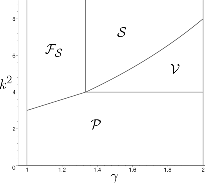
FIG. 1.: Summary of all of the sinks for the Bianchi I magnetic field models in $\{\gamma,k^{2}\}$-parameter space. Note that for each specific pair $\{\gamma,k^{2}\}$, there is a unique sink.

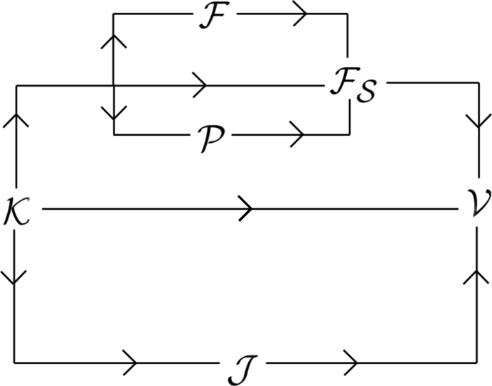
FIG. 2.: Heteroclinic sequences for the Bianchi I models when $\gamma=\frac{5}{3}$, $5<k^{2}<\frac{40}{7}$.

IV Conclusions

We have investigated the class of open Bianchi VI${}_{\mbox{o}}$ universe models with barotropic matter, a scalar field with an exponential potential and a uniform magnetic field. We discussed some of the general properties of the models by utilyzing dynamical systems techniques. The equilibrium point ${\cal P}$ (with $M=0$), corresponding to the power-law inflationary flat FLRW model, is a global sink for $k^{2}<2$. Hence all models are future aymptotic to this inflationary attractor for these parameter values. There is an equilibrium set ${\cal K}$ with $1-\Sigma^{2}_{+}-\Sigma^{2}_{-}-\Phi^{2}=0$ (and $M=0,q=2$), a subset of which are global sources. Hence all models are past asymptotic to massless scalar field models with no matter and no magnetic field.

A (partial) analysis of the saddles was undertaken in order to determine some of the transient features of the models. In particular, we found that there are no equilibrium points with $M\neq 0$ in the Bianchi VI${}_{\mbox{o}}$ state space which are inflationary, and hence concluded that inflation is not fundamentally affected by the presence of a uniform primordial magnetic field in these models.

This latter result is not necessarily inconsistent with the conclusions of Matravers and Tsagas (2000), since only a uniform magnetic field was considered here. Indeed, it is the non-uniform magnetic field gradients that give rise to the magneto-curvature effects in their work which modify the cosmological expansion rate of an almost-FLRW universe and that can have undesirable implications for inflationary models (and may even prevent inflation taking place in the presence of primordial magnetism). It might be thought that on large scales that the magnetic field will be approximately homogeneous, but Matravers and Tsagas (2000) have argued that even weak magetic effects may have significant cosmological consequences. The drawback of their work is that only a local perturbation analysis was performed and questions of genericity and long term behaviour cannot be easily addressed. Clearly, an investigation of the qualitative properties of a class of scalar field cosmological models with an inhomogeneous magnetic field would extend and generalize both the work of Matravers and Tsagas (2000) and the (restricted) analysis of a uniform magnetic field here.

In order to investigate the intermediate behaviour of the models, and hence their physical properties, we discussed the (subset) of Bianchi I models in more detail. We found the equilibrium points ${\cal S}$ and ${\cal V}$, in which all of the matter fields are non vanishing and in which the matter field (only) vanishes, respectively (corresponding to new exact self-similar magnetic field cosmological models), act as sinks in the Bianchi I subset. Heteroclinic sequences (and hence the transient behaviour of the Bianchi I models) were discussed. We found that as $\gamma$ increases, the magnetic field becomes increasingly important at late times.

A

In the main text we followed the dynamical systems theory approach of LeBlanc et al. (1995) to analyse the evolution of orthogonal Bianchi cosmologies of type VI${}_{\mbox{o}}$ with a uniform magnetic field. This approach uses an invariant orthonormal frame in which the commutation functions are the basic variables. Expansion-normalized variables are then introduced, and a reduced set of evolution equations (the dynamical system) for the dimensionless shear variables and spatial curvature variables as well as the dimensionless magnetic field variables and the density parameter are then obtained. All of the equations in the text follow from the analysis of LeBlanc et al. (1995), wherein all quantities are properly defined. However, a coordinate approach is also possible, and it may be of use for the reader to get a better sense of how the equations are derived, at least in the case of the Bianchi I models.

The metric for the class of anisotropic Bianchi I models, which are the simplest spatially homogeneous generalizations of the flat FLRW models which have non-zero shear but zero three-curvature, is given by

$$ds^{2}=-dt^{2}+X^{2}dx^{2}+Y^{2}dy^{2}+Z^{2}dz^{2},$$ (A1)

where $X,Y,Z$ are functions of $t$ only. The expansion rate is given by

$$\theta\equiv 3H=\frac{\dot{X}}{X}+\frac{\dot{Y}}{Y}+\frac{\dot{Z}}{Z},$$ (A2)

and when $Y=Z$ (the LRS subcase) there is only one independent rate of shear, which is given by

$$\sigma=\frac{1}{3}\left(\frac{\dot{Y}}{Y}-\frac{\dot{X}}{X}\right).$$ (A3)

Normalized (dimensionless) variables and a logarithmic time variable $\tau$ are defined by equations (2.3) and (2.4), which then lead to the evolution equations (3.1)-(3.6) in coordinate form (Collins, 1972).

1 Exact Solutions

We can write down the exact solutions corresponding to the equilibrium points ${\cal S}$ and ${\cal V}$ in the text.

• ${\cal S}$: Since $q={\textstyle\frac{3}{2}}\gamma-1$, we can immediately integrate the Raychaudhuri equation $H^{\prime}/H=-(1+q)$ to obtain $H=\frac{2}{3\gamma}t^{-1}$. Since $\Sigma_{-}=0$ and $\Sigma_{+}={\textstyle\frac{1}{4}}(3\gamma-4)$, it follows that $Y=Z$, so that $\sigma=\Sigma_{+}\times H=\frac{1}{2}(1-\frac{4}{3\gamma})t^{-1}$. The metric is consequently of power-law form, viz.,

  $$ds^{2}=-dt^{2}+t^{2p_{1}}dx^{2}+t^{2p_{2}}(dy^{2}+dz^{2}),$$ (A4)

  where $p_{1}$ and $p_{2}$ are constants. From the expressions for $H$ and $\sigma$ we then find that $p_{1}+2p_{2}=\frac{2}{\gamma}$ and $p_{2}-p_{1}=\frac{3}{2}-\frac{2}{\gamma}$ and hence

  $$p_{1}=\frac{2}{\gamma}-1,~{}~{}~{}p_{2}=\frac{1}{2}.$$ (A5)

  The geometry is that of the Jacobs magnetic field model (Jacobs, 1969), and the only difference here is that the matter fields constituting the source are given by

  $$\rho\equiv 3\Omega H^{2}=\left(\frac{4k^{2}-k^{2}\gamma-8\gamma}{2k^{2}\gamma^{2}}\right)t^{-2},~{}~{}~{}~{}H_{1}\equiv 3\sqrt{2}MH=\frac{\sqrt{(2-\gamma)(3\gamma-4)}}{\gamma}t^{-1},$$ (A6)

  and the scalar field is given by

  $$\phi=\phi_{0}-\frac{2}{k}\ln(t),$$ (A7)

  where $\phi_{0}=\frac{1}{k}\ln\left(\frac{2(2-\gamma)}{\gamma k^{2}V_{0}}\right)$. This solution exists provided $\gamma>{\textstyle\frac{4}{3}}$.

• ${\cal V}$: In this solution $q={\frac{5k^{2}-8}{k^{2}+8}}$, so that $H=\frac{k^{2}+8}{6k^{2}}t^{-1}$. $\Sigma_{-}=0$ and $\Sigma_{+}=2{\frac{k^{2}-4}{k^{2}+8}}$, and so the metric is of the form of equation (A4), where now

  $$p_{1}=\frac{8-k^{2}}{2k^{2}},~{}~{}~{}p_{2}=\frac{1}{2}.$$ (A8)

  There is no perfect fluid in this solution ($\rho=0$), and the magnetic field is given by

  $$H_{1}=\frac{\sqrt{\left(k^{2}-4\right)\left(8-k^{2}\right)\left(k^{2}+8\right)}}{k}t^{-1}.$$ (A9)

  The scalar field is given by equation (A7) with $\phi_{0}=\frac{1}{k}\ln\left(\frac{8-k^{2}}{k^{4}V_{0}}\right)$. This new solution exists provided $4\leq k^{2}\leq 8$.

REFERENCES

- [1] B.K. Berger, D. Garfinkle and E. Strasser, 1997, Class. Quantum Grav. 14, L29.
- [2] A.P. Billyard, A.A. Coley, J. Ibañez, I. Olasagasti and R.J. van den Hoogen, 1999, Class. Quantum Grav. 16, 4035.
- [3] C.A. Clarkson and A.A. Coley, 2001, Class. Quantum Grav. 18 1305.
- [4] C.A. Clarkson, A.A. Coley, R. Maartens, and C. G. Tsagas, 2001. In preparation.
- [5] A.A. Coley, Dynamical Systems in Cosmology, in Recent Developments in General Relativity, Proceedings of ERE-99, ed. J. Ibañez, pp. 13-44 [gr-qc/9910074].
- [6] C.B. Collins, 1972, Comm. Math. Phys. 27, 37.
- [7] E.J. Copeland, A.R. Liddle and D. Wands, 1998, Phys. Rev. D 57, 4686.
- [8] K.A. Dunn and B.O.J. Tupper, 1980, Ap. J. 235, 307.
- [9] J. Ehlers, P. Geren, and R. K. Sachs, J. Math. Phys. 9 1344 (1964).
- [10] P.G. Ferreira and M. Joyce, 1997, Phys. Rev. Lett. 79, 4740.
- [11] D. Grasso and H.R. Rubinstein, 2000 (astro-ph/0009061).
- [12] J.J. Halliwell, 1987, Phys. Lett. B185, 341.
- [13] L. Hsu and J. Wainwright, 1986, Class. Quantum Grav. 3, 1105.
- [14] L.P. Hughston and K.C. Jacobs, 1970, Astrophys. J. 160, 147.
- [15] K.C. Jacobs, 1969, Astrophys. J. 155, 379.
- [16] R.T. Jantzen, 1986, Phys. Rev. D 33, 2121.
- [17] Y. Kitada and K. Maeda, 1993 Class. Quantum Grav. 10, 703.
- [18] P.P. Kronberg, J.J. Perry and E.L.H. Zukowski, 1992, Ap. J. 387, 528.
- [19] P.P. Kronberg, 1994, Rep. Prog. Phys. 57, 325.
- [20] V.G. LeBlanc, 1997, Class. Quantum Grav. 14, 2281.
- [21] V.G. LeBlanc, 1998, Class. Quantum Grav. 15, 1607.
- [22] V.G. LeBlanc, D. Kerr and J. Wainwright, 1995, Class. Quantum Grav. 12, 513.
- [23] D. Matravers and C.G. Tsagas, 2000, Phys. Rev. D 62 103519.
- [24] E.N. Parker, 1979, Cosmical Magnetic Fields (Oxford: Oxford University Press).
- [25] S. Quinlan, 2002, Masters Thesis (Dalhousie University).
- [26] C. Tsagas, 2001, Phys. Rev. Lett. 86, in press astro-ph/0012345.
- [27] C.G. Tsagas and J.D. Barrow, 1997, Class. Quantum Grav. 14, 2539.
- [28] C.G. Tsagas and J.D. Barrow, 1998, Class. Quantum Grav. 15, 3523.
- [29] C.G. Tsagas and R. Maartens, 2000, Phys. Rev. D 61, 083519.
- [30] C.G. Tsagas and R. Maartens, 2001, Class. Quantum Grav. 17, 2215.
- [31] J.P. Vallée, 1990a, Astrophys. J. 360, 1.
- [32] J.P. Vallée, 1990b, Astrophys. J. 239, 57.
- [33] J. Wainwright, 2000, Gen. Rel. Grav. 32, 1041.
- [34] J. Wainwright and L. Hsu, 1989, Class. Quantum. Grav. 6, 1409.
- [35] J. Wainwright and G.F.R. Ellis, 1997, Dynamical Systems in Cosmology (Cambridge University Press).
- [36] M. Weaver, 2000, Class. Quantum Grav. 17, 421.
- [37] C. Wetterich, 1988, Nucl. Phys. B 302, 668.
- [38] S. Wiggins, 1990, Introduction to Applied Nonlinear Dynamical Systems and Chaos (New York: Springer).
- [39] A.M. Wolfe, K.M. Lanzetta and A.L. Oren, 1992, Ap. J. 388, 17.