Modeling Galaxy Clustering by Color

Abstract

We extend the mass-halo formalism for analytically generating power spectra to allow for the different clustering behavior observed in galaxy sub-populations. Although applicable to other separations, we concentrate our methods on a simple separation by rest-frame color into “red” and “blue” sub-populations through modifications to the $\langle{\rm N}\rangle(M)$ relations and halo distribution functions for each of the sub-populations. This sort of separation is within the capabilities of the current generations of simulations as well as galaxy surveys, suggesting a potentially powerful observational constraint for current and future simulations. In anticipation of this, we demonstrate the sensitivity of the resulting power spectra to the choice of model parameters.

1 Introduction

The difference in clustering between intrinsically red and blue galaxies has been known since galaxies were first classified into types by Hubble. More recently, the state of cosmological simulations has reached the level where galaxy evolution can be modeled semi-analytically (White & Rees, 1978; White & Frenk, 1991) to produce simulated catalogs with realistic distributions of galaxy colors and types (Kauffmann et al., 1999; Somerville & Primack, 1999; Benson et al., 2000;). Within the framework of these types of simulations, the power spectra and bias of “red” and “blue” galaxies have been measured and found to be in relatively good agreement with previous data measurements. In this paper we seek to derive an analytic method for generating power spectra and biases for these red and blue galaxies from within the mass-halo model.

The first papers developing the revisions of the original mass-halo formalism for dark matter and galaxies focused on real-space correlation functions (Sheth & Jain, 1997; Jing et al., 1998; Peacock & Smith 2000). Recently, these treatments have been extended for the calculation of power spectra (Seljak, 2000; Scoccimarro et al., 2000; Ma & Fry, 2000). Although the results generated by these models closely matched the observed power law behavior for galaxy power spectra (Hamilton et al., 2001), they did not address the observed different clustering within sub-populations. We build on the results from these earlier power spectra treatments to produce physically motivated models for power spectra and biases for galaxy sub-populations. In an effort to keep our model as general as possible, we will refrain from specifying precisely what constitutes a “red” or “blue”galaxy; our approach should work equally well for galaxies separated by type or any other observable with different clustering properties.

In §2, we review the formalism for calculating galaxy power spectra. With this laid out, §3 details the modifications to the halo profiles and the number-mass relation for galaxies populating the halos. Additionally, we work through the modifications to the formulae from §2 necessary to calculate the sub-population power spectra and cross-power spectrum, as well as the associated relative biases. Finally, in §4, we explore the power spectrum space spanned by the new parameters added to the standard model in §3.

2 Calculating Power Spectra

Following the treatment in Seljak, we have four essential ingredients in our galaxy power spectrum: the halo profile, the halo mass function, the halo biasing function, and the galaxy number function. Once these four components are determined, either from observations or simulations, we can fold them together to produce the predicted power spectrum for that particular model.

We begin by generating a halo profile, $\rho(r)$, which is parametrized along the lines of the profile derived by Navarro, Frenk and White (1996; NFW, hereafter),

$$\rho(r)=\frac{\rho_{\rm S}}{\left(r/r_{\rm S}\right)^{-\alpha}\left(1+r/r_{\rm S}\right)^{(3+\alpha)}}$$ (1)

where $r_{\rm S}$ is the universal scale radius and $\rho_{\rm S}=\rho(r_{\rm S})$. In most halo-model treatments, $r_{\rm S}$ is replaced by a concentration, $c\equiv r_{v}/r_{\rm S}$, where $r_{v}$ is the virial radius defining the region where the fractional overdensity of the halo $\delta_{v}$ is approximately 200 and $c$ is a weak function of halo mass ($c\equiv c_{0}(M/M_{*})^{\beta}$, where $c_{0}\sim{\cal O}(10)$ and $\beta\sim-{\cal O}(10^{-1})$). The traditional NFW profile gives $\alpha=-1$, while the Moore profile (Moore et al. 1998) has $\alpha=-3/2$. We will use $\alpha=-1.3$ for the calculations in this paper, but the general results are largely insensitive to the choice of $\alpha$. Bullock (2001) gives $c_{0}=9$ for a pure NFW profile; using Peacock & Smith’s relation, $c_{0}\approx 4.5$ for a Moore profile. Since we are using an intermediate value of $\alpha$, we choose $c_{0}=6$ and $\beta=-0.15$ for all the calculations in this paper. In principle, one can also consider scatter in the concentration at a given mass (Scoccimarro, et al., 2001), leading to an integral over the distribution of $c$, but the magnitude of this effect is small enough that it can be safely ignored.

Rewriting Equation 1 in terms of the concentration and the mass, we get

$$\rho(r,M)=\frac{\rho_{\rm S}}{\left(rc/r_{v}\right)^{-\alpha}\left(1+rc/r_{v}\right)^{3+\alpha}},$$ (2)

where

$$r_{v}^{3} = \frac{3M}{4\pi\delta_{v}\bar{\rho}},$$ (3)

$$\rho_{\rm S} = \frac{\delta_{v}\bar{\rho}c^{3}(M)}{3}\left[\int_{0}^{c(M)}d\chi\frac{\chi^{2+\alpha}}{(1+\chi)^{3+\alpha}}\right]^{-1},$$ (4)

$\bar{\rho}$ is the mean matter density and $M$ is the mass of the halo. Since we will be working in wavenumber space when we generate the power spectrum, we actually need to consider the Fourier transform of the halo profile,

$$y(k,M)=\frac{1}{M}\int_{0}^{r_{v}}4\pi r^{2}\rho(r,M)\frac{\sin(kr)}{kr}dr,$$ (5)

where we have normalized over mass so that $y(0,M)=1$ and $y(k>0,M)<1$. Note that this implies that $\rho(r>r_{v})=0$, truncating the mass integration at the virial radius.

With this in hand, we can move on to the next component of the halo model, the halo mass function, ($dn/dM$). Traditionally, this mass function is expressed in terms of a function $f(\nu)$,

$$\frac{dn}{dM}dM=\frac{\bar{\rho}}{M}f(\nu)d\nu,$$ (6)

where $\nu$ relates the minimum spherical over-density that has collapsed at a given redshift ($\delta_{c}(z)$, $\delta_{c}(0)=1.676$ for an $\Omega_{m}=0.3$, $\Omega_{\Lambda}=0.7$ cosmology) and the rms spherical fluctuations containing mass $M$ ($\sigma(M,z)$) as

$$\nu\equiv\left(\frac{\delta_{c}(z)}{\sigma(M)}\right)^{2}.$$ (7)

We define $M_{*}$ as the mass corresponding to $\nu=1$. The functional form for $f(\nu)$ is traditionally given by the Press-Schechter function (1974). This form tends to over-predict the number of halos below $M_{*}$, so we use the form found from simulations by Sheth and Torman (1997),

$$\nu f(\nu)\sim(1+{\nu^{\prime}}^{-p}){\nu^{\prime}}^{1/2}e^{-{\nu^{\prime}}/2},$$ (8)

where $\nu^{\prime}=a\nu$, $a=0.707$ and $p=0.3$. This relation is normalized by requiring that

$$\frac{1}{\bar{\rho}}\int_{0}^{\infty}\frac{dn}{dM}MdM=\int f(\nu)d\nu=1,$$ (9)

for the dark matter distribution.

On nonlinear scales, we expect the halos to cluster more strongly than the mass, and vice versa for linear scales (Mo & White, 1996). This means we need to positively bias the clustering of the high mass halos relative to the low mass halos. We can generate this sort of halo biasing scheme for the ST mass function using

$$b(\nu)=1+\frac{\nu^{\prime}-1}{\delta_{c}}+\frac{2p}{\delta_{c}(1+{\nu^{\prime}}^{p})}.$$ (10)

In order for the eventual power spectrum to reduce to a linear power spectrum on large scales, we need to impose the further constraint that

$$\int_{0}^{\infty}f(\nu)b(\nu)d\nu=1,$$ (11)

requiring that the biased halos with mass greater than $M_{*}$ be balanced out by anti-biased halos with mass less than $M_{*}$. This integral is satisfied automatically if we use Equation 10 and have properly normalized $f(\nu)$.

Using just these three components, we can generate the power spectrum for the dark matter. However, in order to predict the galaxy power spectrum, we need to know how many galaxies are in a given halo (under the assumption that the distribution of galaxies in the halo follows the halo profile). Currently no theory completely informs the formation of galaxies given a halo mass, but the traditional form of the $\langle{\rm N}\rangle(M)$ relation (Jing et al., 1998; Kauffmann et al., 1999; Benson et al., 2000; White et al., 2001) has the galaxies populating the halo as a simple power law, $\langle{\rm N}\rangle(M)\sim(M/M_{0})^{\gamma}$, where $M_{0}$ sets the unit mass scale and $\gamma<1$. Additionally, one can put in constraints on the minimum mass to form a galaxy and other modifications. For the purposes of the formalism for calculating the power spectrum, however, we can put aside the question of precisely what this function looks like. The inclusion of galaxies does change the normalization of Equation 9 to

$$\int_{0}^{\infty}\frac{\langle{\rm N}\rangle}{M(\nu)}f(\nu)d\nu=\frac{\bar{n}}{\bar{\rho}},$$ (12)

where $\bar{n}$ is the mean number of galaxies.

On large scales, the power spectrum is dominated by correlations between galaxies in separate halos. We need to convolve the halo profile with the mass function to account for the fact that halos are not pointlike objects. Since we are in Fourier space, we can perform the convolution using simple multiplication. The halo-halo power ($P^{hh}_{\rm GG}(k)$) is then simply,

$$P^{hh}_{\rm GG}(k)=P_{\rm LIN}(k)\left[\frac{\bar{\rho}}{\bar{n}}\int_{0}^{\infty}f(\nu)\frac{\langle{\rm N}\rangle}{M(\nu)}b(\nu)y(k,M)d\nu\right]^{2},$$ (13)

where $P_{\rm LIN}(k)$ is the linear dark matter power spectrum. In the small $k$ limit, this reduces to a simple linear bias ($\langle b\rangle$),

$$\langle b\rangle=\frac{\bar{\rho}}{\bar{n}}\int_{0}^{\infty}f(\nu)\frac{\langle{\rm N}\rangle}{M(\nu)}b(\nu)d\nu.$$ (14)

For small scales, the dominant contribution to the power spectrum comes from correlations between galaxies within the same halo. This single halo term is independent of $k$ at larger scales, giving it a Poisson-like behavior. In order to account for the fact that a single galaxy within a halo does not correlate with itself, we use the second moment of the galaxy number relation, ($\langle{\rm N}({\rm N}-1)\rangle$) to calculate the Poisson power ($P^{P}_{\rm GG}(k)$),

$$P^{P}_{\rm GG}(k)=\frac{\bar{\rho}}{(2\pi)^{3}\bar{n}^{2}}\int_{0}^{\infty}f(\nu)\frac{\langle{\rm N}({\rm N}-1)\rangle}{M}|y(k,M)|^{\zeta}d\nu.$$ (15)

Seljak takes $\zeta=2$ for $\langle{\rm N}({\rm N}-1)\rangle>1$ and $\zeta=1$ for $\langle{\rm N}({\rm N}-1)\rangle<1$; this is done to account for the galaxy at the center of the halo in the limit of small number of galaxies. In the limit of large numbers of galaxies, $\langle{\rm N}({\rm N}-1)\rangle$ approaches $\langle{\rm N}\rangle^{2}$, but in the small number limit, $\langle{\rm N}({\rm N}-1)\rangle$ can be approximated by a binomial distribution. This can be implemented by using the fits given in Scoccimarro et al. (2000), letting

$$\langle{\rm N}({\rm N}-1)\rangle=\alpha_{M}^{2}\langle{\rm N}\rangle^{2},$$ (16)

where $\alpha_{M}=1$ for $M>10^{13}h^{-1}M_{\sun}$ and $\alpha_{M}=\log(\sqrt{Mh/10^{11}M_{\sun}})$ for $M<10^{13}h^{-1}M_{\sun}$. Clearly, this will not be exact for an arbitrary $\langle{\rm N}\rangle(M)$, but it should be close enough for our purposes. Adding $P^{hh}_{\rm GG}(k)$ and $P^{P}_{\rm GG}(k)$, we recover the galaxy power spectrum at all wavenumbers, $P_{\rm GG}(k)$.

3 Generating Red & Blue Power Spectra

Within the framework presented above, there are a number of parameters which might be modified to generate models of different power spectra for red and blue galaxies. One could modify the concentration index for each galaxy population, change the halo biasing relation, etc. In this paper, we focus on two modifications to the standard treatment: a modification of the $\langle{\rm N}\rangle$ relations and the halo profiles for each of the galaxy types.

The physical motivation in both of these cases is clear. Semi-analytic models for galaxy formation indicate that the primary determinant of galaxy color is the epoch of initial gas cooling to form the initial stellar population. Red galaxies tend to form earlier, appearing in the deepest over-densities, while the current blue galaxies form later when gas in the shallower potentials and outskirts of the larger potentials has cooled. Given this difference in development, the prospect that the efficiency of galactic formation (and hence number of galaxies produced within a halo of a given local halo mass) would vary for the two epochs is a reasonable conclusion. Likewise, for the different halo profiles, we know from observations as well as simulations that red galaxies tend to populate the centers of galaxy clusters and filaments, while blue galaxies are more numerous at the fringes of structure and in the field. Changing the distribution function for the different colored galaxies within a halo to reflect these observations is an obvious step.

3.1 Modifying $\langle{\rm N}\rangle(M)$

The simplest model we can adopt for the galaxy number relations for the red and blue galaxies ($\langle{\rm N}\rangle_{\rm R}$ and $\langle{\rm N}\rangle_{\rm B}$, respectively) would be the simple power laws alluded to earlier,

$$\langle{\rm N}\rangle_{\rm R}(M)=N_{\rm R0}\left(\frac{M}{M_{\rm R0}}\right)^{\gamma_{\rm R}}$$ (17)

$$\langle{\rm N}\rangle_{\rm B}(M)=N_{\rm B0}\left(\frac{M}{M_{\rm B0}}\right)^{\gamma_{\rm B}}.$$

In practice, this form actually over-determines the functional form of the power laws; since we know the functions pass through unity at some mass scale, we can set $N_{\rm R0}=N_{\rm B0}=1$ and determine the relative contribution of red and blue galaxies by selecting $M_{\rm R0}$ and $M_{\rm B0}$ appropriately.

Such a model does reasonably well, but the GIF simulations (Kauffmann, et al., 1999) point to an extra abundance of blue galaxies at small halo masses ($M\sim 10^{12}h^{-1}M_{\sun}$). Sheth et al. (2001) include this effect by the addition of a Gaussian term to the $\langle{\rm N}\rangle_{\rm B}$ relation,

$$\langle{\rm N}\rangle_{\rm B}(M)=\left(\frac{M}{M_{\rm B0}}\right)^{\gamma_{\rm B}}+Ae^{-4(\log(M)-M_{\rm Bs})^{2}},$$ (18)

where $A$ is ${\cal O}(1/2)$ and $M_{\rm Bs}$ is the logarithm of the mass corresponding to the peak in the Gaussian component. All told, this gives us six tunable parameters for the $\langle{\rm N}\rangle$ relations. For the purposes of our power spectrum calculations, we will add an additional lower mass cut-off for the $\langle{\rm N}\rangle_{\rm R}$ relations at $10^{11}h^{-1}M_{\sun}$; the resulting power spectra are not terribly sensitive to the precise value of this cut-off.

3.2 Modifying Halo Profiles

In modifying the distribution functions for red and blue galaxies, we have a number of constraints. First, we require that the sum of the matter associated with red galaxies and that with blue galaxies match the total distribution of matter at all halo radii. This is not to say that all the matter ends up in galaxies; rather, it merely requires that the combined distribution of red and blue galaxies in the halo match the total galaxy distribution. Although this would appear to suppress natural correlations between red and blue galaxies, Sheth & Lemson (1999) show that this sort of clustering by conservation of number works reasonably well.

There are any number of profiles we might choose to consider for the red and blue sub-profiles. In principle, the shapes of these profiles could be found from analyzing the results of simulations, but for the purposes of this exercise we will forgo that complication. Instead, we will restrict ourselves to profiles of a similar form as that given in Equation 1 with different values of $\rho_{\rm S}$ and $\alpha$ for the red and blue sub-populations. Of course, the sum of two profiles with differing values of $\alpha$ do not quite match a profile with a third value of $\alpha$, but we can come reasonably close with clever choices of $\alpha_{\rm R}$ and $\alpha_{\rm B}$ for the red and blue populations, respectively.

In order to find the proper values for our extended halo parameter set, we need only know the relative abundance of red and blue galaxies at two points along the radial profile. At large radii relative to the virial radius, all of the profiles go as $\rho\sim r^{-}3$, meaning that the ratio of the number of blue galaxies to red galaxies ($\eta$) in this regime gives us the ratio of $\rho_{\rm SB}/\rho_{\rm SR}$ immediately, once we have transformed from number of galaxies to mass assigned to galaxies (see below). We consider the halos truncated at these large radii when we calculate the power spectra, but this allows us to set the relative normalization of $\rho_{\rm SR}$ and $\rho_{\rm SB}$ under the assumption that $\eta$ does not vary much beyond $r_{v}$.

With this ratio determined, the choice of the second radial point is somewhat arbitrary, but clearly we would prefer this point to be at very small radius where the profiles go as $\rho\sim r^{\alpha}$. For all of the calculations, we set the inner radius such that $r_{i}c/r_{v}=0.1$. This demands a resolution smaller than most simulations can provide at the moment, but does guarantee that we are well into the $\rho\sim r^{\alpha}$ regime.

For a given ratio ($\mu$) of red to blue galaxies at small radius, the difference in $\alpha$ for the red and blue profiles is

$$\Delta\alpha\equiv\alpha_{\rm B}-\alpha_{\rm R}=\frac{\log(\mu\eta)}{\log(1+r_{i}c/r_{v})-\log(r_{i}c/r_{v})},$$ (19)

where we have assumed that the mass follows the number of galaxies linearly. However, to properly conserve the mass in the halo, we need to transform $\mu$ and $\eta$ into mass-space using the $\langle{\rm N}\rangle$ functions for the red and blue galaxies to yield $\mu^{\prime}$ and $\eta^{\prime}$, respectively. In the absence of the Gaussian term in the $\langle{\rm N}\rangle_{\rm B}$ relation, these transform as

$$\eta^{\prime} = \eta^{1/\gamma_{\rm B}}\frac{M_{\rm B0}}{M_{\rm R0}}$$ (20)

$$\mu^{\prime} = \mu^{1/\gamma_{\rm R}}\frac{M_{\rm R0}}{M_{\rm B0}}.$$

If we wish to include the Gaussian term, a bit of algebra gives the slightly more complex form of the transformation:

$$\eta^{\prime} = \left[\eta-Ae^{-4(\log(M_{\rm R0})-M_{\rm Bs})^{2}}\right]^{1/\gamma_{\rm B}}\frac{M_{\rm B0}}{M_{\rm R0}}$$ (21)

$$\mu^{\prime} = \left[\mu\left(1+Ae^{-4(\log(M_{\rm B0})-M_{\rm Bs})^{2}}\right)\right]^{1/\gamma_{\rm R}}\frac{M_{\rm R0}}{M_{\rm B0}}.$$

As one might expect, the limit that $M_{\rm R0},M_{\rm B0}\gg 10^{M_{\rm Bs}}$, Equation 21 effectively reduces to Equation 20. Once we have made this transformation, we then replace $\mu$ and $\eta$ in Equation 19 with $\mu^{\prime}$ and $\eta^{\prime}$. With this relation between $\alpha_{\rm R}$ and $\alpha_{\rm B}$ in hand, we can perform a simple search over values of $\alpha_{\rm R}$ to find the sub-profiles that combine to closest match an overall profile with a given value of $\alpha$. Since we know that $\Delta\alpha$ must be positive, this relation guarantees a flatter distribution of blue galaxies in the center of halos relative to red galaxies, something which would be much more difficult to accomplish had we varied $c$ for the differ galaxy populations.

Using $\rho_{\rm SR}$, $\rho_{\rm SB}$, $\alpha_{\rm R}$ and $\alpha_{\rm B}$, where

$$\rho_{\rm SR} = \frac{1}{\eta^{\prime}+1}\rho_{\rm S}$$ (22)

$$\rho_{\rm SB} = \frac{\eta^{\prime}}{\eta^{\prime}+1}\rho_{\rm S},$$

we can recalculate $y(k,M)$ along the lines of Equation 5, making $y_{\rm R}$ and $y_{\rm B}$. We can also recover the distribution of galaxies by color/type within a given halo similar to that seen in simulations (cf. Diaferio et al., 1999), as seen in Figure 1. Clearly, the agreement is not perfect, but it is close enough that we can proceed with confidence that the basic approach is reasonable. These diagrams inform our fiducial choices of $\mu$ and $\eta$ such that $\mu\sim{\cal O}(10)$ and $\eta\sim{\cal O}(\sqrt{(}10))$; for our models we take $\mu=10$ and $\eta=4$.

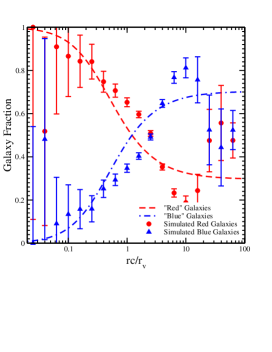
Figure 1: Fraction of “red” and “blue” galaxies as a function of $rc/r_{v}$ compared to the distribution of galaxies from the GIF simulations. For the simulated data, red galaxies were taken to have $g^{\prime}-r^{\prime}<0.6$ in the rest frame for SDSS magnitudes (Fukugita, et al. 1996).

3.3 Calculating Subpopulation Power Spectra and Biases

Plugging all this into the standard formalism, we can calculate the power spectra for these galaxy populations, as well as their cross-correlation, in the same manner as described in Seljak. In order to calculate the power spectra properly, we need to re-normalize $f(\nu)$ for each sub-population using Equation 12 to account for the differences in $\langle{\rm N}\rangle$ and $\bar{n}$:

$$\int_{0}^{\infty}\frac{\langle{\rm N}\rangle_{\rm R}}{M(\nu)}f_{\rm R}(\nu)d\nu = \frac{\bar{n}_{\rm R}}{\bar{\rho}}$$ (23)

$$\int_{0}^{\infty}\frac{\langle{\rm N}\rangle_{\rm B}}{M(\nu)}f_{\rm B}(\nu)d\nu = \frac{\bar{n}_{\rm B}}{\bar{\rho}}$$

Once this has been done, we can insert the above (along with the color-dependent halo profiles) into Equations 13 and 15 to generate the power spectra for red and blue galaxies:

$$\frac{P^{hh}_{\rm RR}(k)}{P_{\rm LIN}(k)}=\left[\frac{\bar{\rho}}{\bar{n}_{\rm R}}\int_{0}^{\infty}f_{\rm R}(\nu)\frac{\langle{\rm N}\rangle_{\rm R}}{M(\nu)}b(\nu)y_{\rm R}(k,M)d\nu\right]^{2}$$ (24)

$$P^{P}_{\rm RR}(k)={\bar{\rho}}\int_{0}^{\infty}f_{\rm R}(\nu)\frac{\langle{\rm N}({\rm N}-1)\rangle_{\rm R}}{(2\pi)^{3}\bar{n}_{\rm R}^{2}M(\nu)}|y_{\rm R}(k,M)|^{\zeta}d\nu,$$

$$\frac{P^{hh}_{\rm BB}(k)}{P_{\rm LIN}(k)}=\left[\frac{\bar{\rho}}{\bar{n}_{\rm B}}\int_{0}^{\infty}f_{\rm B}(\nu)\frac{\langle{\rm N}\rangle_{\rm B}}{M(\nu)}b(\nu)y_{\rm B}(k,M)d\nu\right]^{2}$$

$$P^{P}_{\rm BB}(k)=\bar{\rho}\int_{0}^{\infty}f_{\rm B}(\nu)\frac{\langle{\rm N}({\rm N}-1)\rangle_{\rm B}}{(2\pi)^{3}\bar{n}_{\rm B}^{2}M(\nu)}|y_{\rm B}(k,M)|^{\zeta}d\nu.$$

As before, we generate the total power spectra ($P_{\rm RR}(k)$ and $P_{\rm BB}(k)$) by taking the sum of these parts,

$$P_{\rm RR}(k) = P^{hh}_{\rm RR}(k)+P^{P}_{\rm RR}(k)$$ (25)

$$P_{\rm BB}(k) = P^{hh}_{\rm BB}(k)+P^{P}_{\rm BB}(k).$$

To generate the cross-power spectrum, we take one factor from each of the different power spectrum terms. This makes the halo-halo term

$$\frac{P^{hh}_{\rm RB}(k)}{P_{\rm LIN}(k)} = \left[\frac{\bar{\rho}}{\bar{n}_{\rm R}}\int_{0}^{\infty}f_{\rm R}(\nu)\frac{\langle{\rm N}\rangle_{\rm R}}{M(\nu)}b(\nu)y_{\rm R}(k,M)d\nu\right]\times$$ (26)

$$\left[\frac{\bar{\rho}}{\bar{n}_{\rm B}}\int_{0}^{\infty}f_{\rm B}(\nu)\frac{\langle{\rm N}\rangle_{\rm B}}{M(\nu)}b(\nu)y_{\rm B}(k,M)d\nu\right].$$

For the Poisson term, we simply replace the second moment of the galaxy number relations with the product of $\langle{\rm N}\rangle_{\rm R}$ and $\langle{\rm N}\rangle_{\rm B}$,

$$P^{P}_{\rm RB}(k)=\bar{\rho}\int_{0}^{\infty}\bar{f}(\nu)\frac{\langle{\rm N}\rangle_{\rm R}\langle{\rm N}\rangle_{\rm B}}{(2\pi)^{3}\bar{n}_{\rm R}\bar{n}M(\nu)}|\bar{y}(k,M)|^{\zeta}d\nu,$$ (27)

where $\bar{f}(\nu)$ and $\bar{y}(k,M)$ are the geometric means of the red and blue values.

The results of such a calculation are shown in Figure 2. For our fiducial model, we choose the set of input parameters in a $\Lambda{\rm CDM}$ model given in Table 1. As we would generally expect, the red galaxies show a stronger biasing than either the total sample or the blue sample, as well as tracing the shape of the dark matter power spectrum ($P_{\rm DD}(k)$) more closely. The blue galaxies are anti-biased relative to the normal galaxy power spectrum, and demonstrate a slightly steeper slope. Additionally, the blue galaxies demonstrate a sharp break from a power law at small scales. This effect is due solely to the $\langle{\rm N}\rangle(M)$ relation for the blue galaxies and not the halo profiles; the larger number of blue galaxies in smaller, less massive halos sets in at this scale, driving the power up. Remarkably, however, the galaxy populations that generate these power spectra combine to produce a total galaxy power spectrum with simple power law behavior. The exact comparison of these predicted power spectra to those from simulations we leave as a detail for future work; for now we are more interested in the flexibility of the model than precise values for parameters.

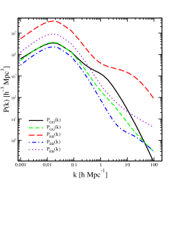
Figure 2: Power spectra for red ($P_{\rm RR}(k)$) and blue ($P_{\rm BB}(k)$) galaxies and their cross-power spectrum ($P_{\rm RB}(k)$) compared to the dark matter ($P_{\rm DD}(k)$) and galaxy ($P_{\rm GG}(k)$) power spectra.

Table 1: Fiducial model parameters for power spectra in Figure 2

Description	Parameter	Value
Red Unit Mass Scale	$M_{\rm R0}$	$3\times 10^{12}h^{-1}M_{\sun}$
Blue Unit Mass Scale	$M_{\rm B0}$	$7\times 10^{13}h^{-1}M_{\sun}$
Red Mass Scaling Index	$\gamma_{\rm R}$	0.9
Blue Mass Scaling Index	$\gamma_{\rm B}$	0.7
Gaussian Normalization	$A$	0.5
Gaussian Mass Scale	$M_{\rm Bs}$	11.75
Outer Galaxy Ratio	$\eta$	4
Inner Galaxy Ratio	$\mu$	10

With this machinery in place, we can calculate the relative bias between the various power spectra:

$$b_{\rm RB}(k)^{2}=\frac{P_{\rm RR}(k)}{P_{\rm BB}(k)} b_{\rm RG}(k)^{2}=\frac{P_{\rm RR}(k)}{P_{\rm GG}(k)}$$ ; (28)

$$b_{\rm BG}(k)^{2}=\frac{P_{\rm BB}(k)}{P_{\rm GG}(k)} b_{\rm RBG}(k)^{2}=\frac{P_{\rm RB}(k)}{P_{\rm GG}(k)}.$$ ;

We choose relative biases between the various galaxy power spectra rather than the absolute biases relative to the dark matter for two reasons. First, in each of the cases in §4 where we vary a parameter in our model, at least one of $P_{\rm GG}(k)$, $P_{\rm RR}(k)$ or $P_{\rm BB}(k)$ remains roughly constant, so we can use that power spectrum as a baseline for seeing how the other one or two vary. Second, while the absolute biases can be measured using galaxy magnification bias, the relative biases involve real clustering that can be measured over a much wider range of redshift for a given photometric or spectroscopic survey (the evolution of these biases over redshift will be left for future work).

As with the results calculated by Seljak, the relative biases shown in Figure 3 are constant on large scales, whereas on small scales there is considerable variation, particularly in the $b_{\rm RB}(k)$ and $b_{\rm BG}(k)$ biases. As we will see later, the behavior of these biases is a strong function of the model input, suggesting that reasonably small error bars on the the bias in wavenumber space could act as a powerful constraint on the model parameters.

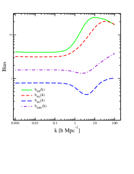
Figure 3: Relative biases between red and blue galaxies ($b_{\rm RB}(k)$) and the red, blue and cross power spectra and the galaxy power spectrum ($b_{\rm RG}(k)$, $b_{\rm BG}(k)$, and $b_{\rm RBG}(k)$, respectively).

4 Variations

4.1 Inner and Outer Ratios

As Equations 19 and 21 suggest, the effect of our choices for $\eta$ and $\mu$ will be at least partially determined by the ratio of $M_{\rm R0}/M_{\rm B0}$. In the regime where $M_{\rm B0}\gg M_{\rm R0}$ as in the fiducial model, the actual values of $\mu$ and $\eta$ are not so important to the resulting power spectra as their product. Likewise, since the profile that the blue galaxies will populate is relatively flat in the center of each halo, the effects of changing the value of $\mu\eta$ does not significantly change the clustering of the blue galaxies; the majority of the mass associated with normal NFW profiles is outside the $\rho\sim r^{\alpha}$ region anyway and, since $\alpha_{\rm B}>\alpha$ by construction, this will be even more pronounced for the blue galaxies. Thus, we do not expect $P_{\rm BB}(k)$ to vary significantly with $\mu\eta$ and we have constructed $\alpha_{\rm R}$ and $\alpha_{\rm B}$ such that $P_{\rm GG}(k)$ will not vary, so the only sensitivity to $\mu\eta$ we expect to see is in $P_{\rm RR}(k)$ and $P_{\rm RB}(k)$ and the associated relative biases. In Figure 4, we show $b_{\rm RG}(k)$ for several different values of $\mu\eta$. There is some change in the shape of the bias, perhaps indicative of a more negative $\alpha_{\rm R}$ in the high $\mu\eta$ models leading to a greater population of the inner regions of the halos with red galaxies. Indeed, in most of these models, the matter associated with red galaxies only exceeds that associated with blue galaxies in the very inner regions of the halo.

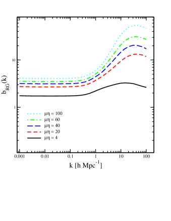
Figure 4: $b_{\rm RG}(k)$ for several values of $\mu\eta$ in the limit where $M_{\rm B0}\gg M_{\rm R0}$. $P_{\rm GG}(k)$ and $P_{\rm BB}(k)$ are unaffected by changes in $\mu\eta$ in this limit.

In a model where $M_{\rm B0}\approx M_{\rm R0}$, the degeneracy between $\mu$ and $\eta$ is broken. Figure 5 shows $b_{\rm RG}(k)$ and $b_{\rm BG}(k)$ for two models where $M_{\rm B0}=M_{\rm R0}=3\times 10^{12}h^{-1}M_{\sun}$ and $\mu\eta=40$. Since Equations 19 and 22 are no longer dominated by the ratio of $M_{\rm R0}/M_{\rm B0}$, we can see significant shifts in the biases of both red and blue galaxies relative to $P_{\rm GG}(k)$. In this case, we have a more equal distribution between the mass associated with red and blue galaxies and less extreme relative halo profile normalizations. Clearly, using future measurements to constrain these parameters will require using multiple biases to minimize these degeneracies.

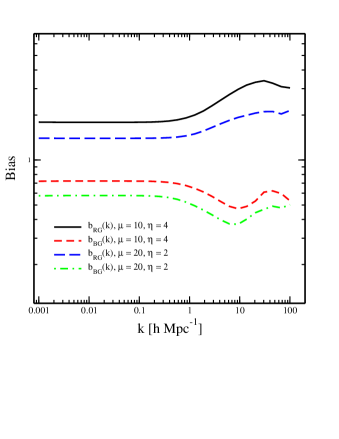
Figure 5: $b_{\rm RG}(k)$ and $b_{\rm BG}(k)$ for equal values of $\mu\eta$ in the $M_{\rm R0}\approx M_{\rm B0}$ regime. $P_{\rm GG}(k)$ remains constant for all values of $\mu\eta$ by construction.

4.2 $\langle{\rm N}\rangle$(M) Relations

Unlike modifying the halo profiles, changing the parameters in the $\langle{\rm N}\rangle(M)$ relations can have significant effects on the shapes of all the power spectra not just $P_{\rm RR}(k)$ and $P_{\rm BB}(k)$. The general effect of each of the modifications is to change the behavior of the Poisson term in the power spectra, but the specific effects for each modification show considerable and sometimes surprising variations.

We begin with the unit mass scale for the blue galaxies, $M_{\rm B0}$. In general, this parameter does not strongly affect the total galaxy power spectrum; there is some slight variation ($\sim 5\%$) over the range $10^{12}h^{-1}M_{\sun}<M_{\rm B0}<10^{14}h^{-1}M_{\sun}$ in the quasi-linear regime of the power spectrum ($k\approx hMpc^{-1}$). However, there is significant change in the relative biases of the red and blue galaxies, as shown in Figure 6. Additionally, as $\log(M_{\rm B0})$ approaches $M_{\rm Bs}$, the non-power law behavior of $P_{\rm BB}(k)$ is considerably damped out.

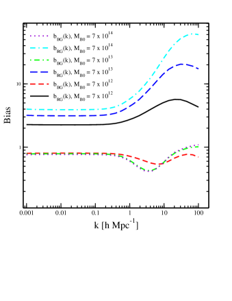
Figure 6: $b_{\rm RG}(k)$ and $b_{\rm BG}(k)$ for several values of $M_{\rm B0}$. Masses are given in $h^{-1}M_{\sun}$. $P_{\rm GG}(k)$ remains constant over variations in $M_{\rm B0}$.

In contrast to $M_{\rm B0}$, modifying the values of $M_{\rm R0}$ leads to large variations in the shape and amplitude of $P_{\rm GG}(k)$, with lesser amplitude shifts to $P_{\rm RR}(k)$ and almost no effect on $P_{\rm BB}(k)$ (as we might suspect). Figure 7 shows $b_{\rm RB}(k)$ and $b_{\rm BG}(k)$ for a two decade range in $M_{\rm R0}$ values. As $M_{\rm R0}$ approaches $M_{\rm B0}$, the effect of the Gaussian term in $\langle{\rm N}\rangle_{\rm B}$ on $P_{\rm GG}(k)$ increases, leading to a galaxy power spectrum with a strong break in its power law at large wavenumber. Conversely, at lower $M_{\rm R0}$, the galaxy power spectrum inflects, leading to a stronger anti-bias in $P_{\rm BB}(k)$ relative to $P_{\rm GG}(k)$ around $k\sim 1$. Additionally, in this limit we can see the effect of the Gaussian component in the transformation from $\eta$ to $\eta^{\prime}$ (Equation 21) changing the effective value of $\mu\eta$.

Figure 7: $b_{\rm RB}(k)$ and $b_{\rm BG}(k)$ for several values of $M_{\rm R0}$. Masses are given in $h^{-1}M_{\sun}$. $P_{\rm BB}(k)$ is constant over this range in $M_{\rm R0}$.

Due to the sub-dominant role of $\langle{\rm N}\rangle_{\rm B}$ to that of $\langle{\rm N}\rangle_{\rm R}$ over most of the mass range, varying $\gamma_{\rm B}$ does not significantly change any of the power spectra. Changing $\gamma_{\rm R}$ alters $P_{\rm RR}(k)$ and $P_{\rm GG}(k)$ slightly, generally smoothing out the variations in $b_{\rm RG}(k)$ over $k$ for larger values of $\gamma_{\rm R}$.

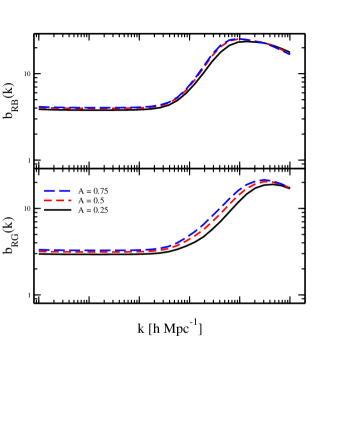
Figure 8: $b_{\rm RB}(k)$ and $b_{\rm RG}(k)$ for several values of $A$. $P_{\rm RR}(k)$ is unaffected by our choice of $A$.

Changing $A$ and $M_{\rm Bs}$ has minimal effect on the red power spectrum, so long as we are in the $M_{\rm R0},M_{\rm B0}\gg 10^{M_{\rm Bs}}$ regime. There are, however, effects on $P_{\rm GG}(k)$ and $P_{\rm BB}(k)$ (quite strong effects in the case of $M_{\rm Bs}$) and we can begin to see our approximation neglecting the Gaussian term in Equation 20 break down as $M_{\rm Bs}$ approaches $M_{*}$, resulting in biased $P_{\rm BB}(k)$ relative to $P_{\rm GG}(k)$ at small scales. Increasing the value of $A$ has a slight global effect on $b_{\rm RB}(k)$ and $b_{\rm RG}(k)$ (Figure 8), but mostly it controls the on-set of the break in the $P_{\rm BB}(k)$ power-law with large values of $A$ lead to a sharper break. The mass scale for the contribution of the Gaussian term in $\langle{\rm N}\rangle_{\rm B}$ plays a much more significant role. Large values of $M_{\rm Bs}$ increase $P_{\rm BB}(k)$ (and, to a lesser extent, $P_{\rm GG}(k)$) on all scales, leading to a suppression of $b_{\rm RB}(k)$ and $b_{\rm RG}(k)$ as $M_{\rm Bs}$ increases (Figure 9). Likewise, as the mass of the halos experiencing this boost in $P^{P}_{\rm BB}(k)$ increases, the onset of the bump in the power law for $P_{\rm BB}(k)$ occurs on larger and larger scales.

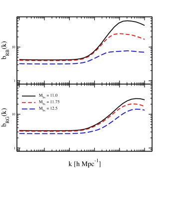
Figure 9: $b_{\rm RB}(k)$ and $b_{\rm RG}(k)$ for several values of $M_{\rm Bs}$. Again, $P_{\rm RR}(k)$ remains constant for different values of $M_{\rm Bs}$.

As mentioned above, the over-riding theme of these variations appears to be the effect of changing at what scale and in what way the Poisson contribution to the power spectra sets in. As $M_{\rm B0}$ and $M_{\rm R0}$ increase, fewer galaxies resulting from the power law parts of $\langle{\rm N}\rangle_{\rm B}$ and $\langle{\rm N}\rangle_{\rm R}$ populate the lower mass halos and small scale power-law behavior is suppressed in favor of the Gaussian contribution to $\langle{\rm N}\rangle_{\rm B}$. The degree to which this non-power law behavior in the red and blue galaxies is recreated in the data and simulations should be an excellent clue as to setting the relative amplitude of $M_{\rm B0}$ and $M_{\rm R0}$ as well as $M_{\rm Bs}$.

5 Conclusion

We have shown that, through relatively simple modifications to the $\langle{\rm N}\rangle$ and halo profile relations in the standard formalism, we can generate reasonable power spectra for red and blue galaxies, as well as a number of relative biases between the various galaxy power spectra. By manipulation of the parameters constituting the $\langle{\rm N}\rangle$ relations, we have considerable ability to modify the shapes of the red and blue power spectra. Likewise, in the limit where we are not dominated by the $\langle{\rm N}\rangle$ relations, our choice of halo profile parameters allows us to set the relative large-scale biases between the various power spectra over a large range, while keeping the shapes of the power spectra relatively constant. There is some degree of degeneracy between the choice of $M_{\rm B0}$ & $M_{\rm R0}$ and the halo profiles for each of the galaxy sub-populations, suggesting that a simple fit to $\langle{\rm N}\rangle$ from simulations without including this effect could result in an apparently larger difference between the two mass scales than the data actually indicate. Still, the degree of flexibility within the framework and sensitivity to the various input parameters suggest that measurements of these relative biases using current large galaxy survey data will provide strong constraints on these input parameters and the outputs of simulations.

6 Acknowledgments

Many thanks to Scott Dodelson and Ravi Sheth for useful advice and editing comments and thanks to Gilbert Holder for many insightful conversations. Additional thanks to Guinevere Kaufmann, Volker Springel and Antonaldo Diaferio for assistance with the simulation data.

Support for this work was provided by the NSF through grant PHY-0079251 as well as by NASA through grant NAG 5-7092 and the DOE.

7 References

Benson, A.J., Cole, S., Frenk, C.S., Baugh, C.M., & Lacey, C.G. 2000, MNRAS , 311, 793

Bullock, J. S., Kolatt, T. S., Sigad, Y., Somerville, R. S., Kravtsov, A. V., Klypin, A. A., Primack, J. R., Dekel, A. 2001, MNRAS , 321, 559

Diaferio, A., Kauffmann, G., Colberg, J.M., & White, S.D.M. 1999, MNRAS , 307, 537

Hamilton, A. J. S., Tegmark, M., Padmanabhan, N. 2000, MNRAS , 317, 23

Fukugita, M., Ichikawa, T., Gunn, J.E., Doi, M., Shimasaku, K., & Scheider, D.P., 1996, AJ, 111,1748

Kauffmann, G., Colberg, J.M., Diaferio, A. & White, S.D.M. 1999, MNRAS , 303, 188

Jing, Y.P., Mo, H.J., Borner, G. 1998, ApJ , 499,20

Ma, C.-P. & Fry, J.N., ApJ , 543, 503

Mo, H.J., White, S.D.M 1996, MNRAS , 282, 1096

Moore, B., Governato, F., Quinn, T., Stadel, J., & Lake, G. 1999, MNRAS , 261, 827

Navarro, J., Frenk, C., & White, S.D.M. 1996, ApJ , 462, 563 Ap. J. Let. 499, L5

Peacock, J.A. & Smith, R.E. 2000, MNRAS , 318, 1144

Press, W.H. & Schechter, P. 1974, ApJ , 187, 425

Seljak, U. 2000, MNRAS , 318, 203

Sheth, R., Diaferio, A., Hui, L., Scoccimarro, R. 2001, MNRAS , 326, 463

Sheth, R., Lemson, G. 1999, MNRAS , 304, 767

Sheth, R. & Tormen, G. 1999, MNRAS , 308, 119

Scoccimarro, R., Sheth, R.K., Hui, L. & Jain, B. 2001, ApJ , 546, 20

Somerville, R.S. & Primack, J.R. 1999, MNRAS , 310, 1087

White, M., Hernquist, L., Springel, V. 2001, ApJ , 550, 129

White, S.D.M & Frenk, C.S. 1991, ApJ , 379, 52

White, S.D.M & Rees, M.J. 1978, MNRAS , 183, 341