Abstract

After a brief introduction to gravitational lensing theory, a rough overview of the types of gravitational lensing statistics that have been performed so far will be given. I shall then concentrate on recent results of galaxy-galaxy lensing, which indicate that galactic halos extend much further than can be probed via rotation of stars and gas.

1 Introduction

Since I am the first at this meeting who talks about gravitational lensing (GL), I thought it might be useful if I start by recalling some of the basics of GL-theory and standard terminology.
Space does not allow me to discuss in any detail the types of lensing statistics that have been performed so far. After a brief discussion of the main ones, I shall concentrate on some recent studies of galaxy-galaxy lensing which have led to some interesting -although not definite- results on the properties of galactic halos. The existing measurements demonstrate the power and potential of this method. The data indicate that halos of typical galaxies continue an isothermal profile to a radius of at least 260 h${}_{o}^{-1}$ kpc, but in the foreseeable future the situation should improve considerably.

2 Basics of Gravitational Lensing Theory

Gravitational lensing has the distinguishing feature of being independent of the nature and the physical state of the deflecting mass distributions. Therefore, it is perfectly suited to study dark matter on all scales.
Moreover, the theoretical basis of lensing is very simple. For all practical purposes we can use the ray approximation for the description of light propagation. In this limit the rays correspond to null geodesics in a given gravitational field. For a qualitative understanding it is helpful to use the Hamilton-Jacobi description of ray optics. Let me briefly recapitulate how this looks in general relativity (see e.g. Straumann 1999).
If we insert the following eikonal ansatz for the Maxwell field

$$F_{\mu\nu}\,=\,{\cal R}e\Bigl{(}f_{\mu\nu}\,e^{iS}\Bigr{)},$$

with a slowly varying amplitude $f_{\mu\nu}$ and a real $S$ into the general relativistic Maxwell equations, we obtain the eikonal equation

$$g^{\mu\nu}\,\partial_{\mu}S\partial_{\nu}S\,=\,0.$$ (1)

This says that the vector field $k^{\mu}(x)=\nabla^{\mu}S$ is null. The integral curves of $k^{\mu}(x)$ are the light rays. From the general relativistic eikonal equation (1) one easily shows that they are -as expected- null geodesics. By construction they are orthogonal to the wave fronts $S=const$.
For an almost Newtonian situation the metric is ($c=1$):

$$g_{\mu\nu}dx^{\mu}dx^{\nu}\,=\,-(1+2U)dt^{2}+(1-2U)d\mathbf{x}^{2},$$ (2)

where $U$ is the Newtonian potential. Since this is time independent, we can make the ansatz

$$S(x)\,=\,\widehat{S}(\mathbf{x})-\omega t$$ (3)

and obtain for $\widehat{S}(\mathbf{x})$ the standard eikonal equation of geometrical optics

$$(\bm{\nabla}\widehat{S})^{2}\,=\,n^{2}\omega^{2},$$ (4)

with the effective refraction index

$$n(\mathbf{x})\,=\,1-2U(\mathbf{x})/c^{2}.$$ (5)

This shows that in the almost Newtonian approximation general relativity implies that gravitational lensing theory is just usual ray optics with the effective refraction index (5). (In a truely cosmogical context, things are not quite that simple).
At this point the qualitative picture sketched in Fig.1 is useful for a first orientation. It shows the typical structure of wave fronts in the presence of a cluster perturbation, as well as the rays orthogonal to them.

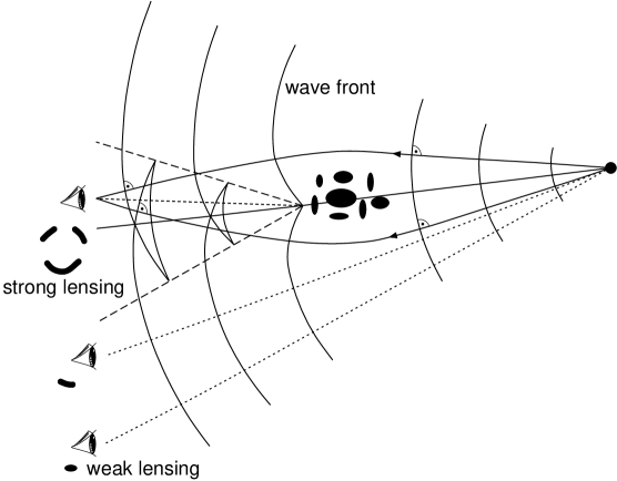
Figure 1: Wave fronts and light rays in the presence of a cluster perturbation.

For sufficiently strong lenses the wave fronts develop edges and self-interactions. An observer behind such folded fronts obviously sees more than one image. From this figure one also understands how the time delay of pairs of images arises: this is just the time elapsed between crossings of different sheets of the same wave front. Since this time difference is, as any other cosmological scale, depending on the Hubble parameter, GL provides potentially a very interesting tool to measure the Hubble parameter. So far, the uncertainties of this method are still quite large, but the numbers fall into a reasonable range.
If the extension of a lens is much smaller than the distances between the lens and the observer as well as the source, one can derive the following equation for the lens map (Schneider et al 1992, Straumann 1999): Adopting the notation in Fig.2, the map $\varphi$: $\bm{\theta}\mapsto\bm{\beta}$ (image $\rightarrow$ source) is the gradient map:

$$\varphi(\bm{\theta})\,=\,\bm{\nabla}\Bigl{(}\frac{1}{2}\bm{\theta}^{2}-\psi(\bm{\theta})\Bigr{)},$$ (6)

where the deflection potential $\psi$ satisfies the two-dimensional Poisson equation

$$\Delta\psi\,=\,2\kappa.$$ (7)

Here, $\kappa$ is the projected mass density $\Sigma(\bm{\theta})$ in units of the critical surface mass density. (The latter is defined such that if $\kappa>1$ somewhere there are always multiple images for some source positions.)

Figure 2: Notation adopted for the description of the lens geometry.

The linearized lens map

$${\cal A}\,=\,\Bigl{(}\delta_{ij}-\frac{\partial^{2}\psi}{\partial\theta_{i}\partial\theta_{j}}\Bigr{)}$$ (8)

is usually parametrized as

$${\cal A}\,=\,\left(\begin{array}[]{cc}1-\kappa-\gamma_{1}&-\gamma_{2}\\ -\gamma_{2}&1-\kappa+\gamma_{1}\end{array}\right).$$ (9)

Note that the complex shear $\gamma=\gamma_{1}+i\gamma_{2}$ describes the trace-free part of ${\cal A}$ and does, therefore, not transform like a vector.
Let me also recall how $\gamma$ can be measured in the limit of weak lensing. Knowing the surface brightness distribution $I(\bm{\theta})$ of a galaxy image allows us to compute the tensor $Q_{ij}$ of brightness moments and thus the complex ellipticity

$$\epsilon\,=\,\frac{Q_{11}-Q_{22}+2iQ_{12}}{{\rm tr}Q+2{\rm det}Q}.$$ (10)

By making use of (9) one find for weak lensing ($\kappa\ll 1$) the following relation between $\epsilon$ and the corresponding source ellipticity $\epsilon^{(s)}:\epsilon=\epsilon^{(s)}+\gamma$. For an individual galaxy this is, of course, not of much use, but for a sufficiently dense ensemble it is reasonable to assume that the average value $<\epsilon^{(s)}>$ vanishes. One can, however, not exclude some intrinsic alignments of galaxies caused, for instance, by tidal fields. This can be tested, as I shall discuss later. If we set $<\epsilon^{(s)}>=0$ we have $\gamma=<\epsilon>$, and $\gamma$ can thus be measured.

3 Types of Lensing Statistics

I confine myself just to a few remarks on statistics involving strong lensing, because in all cases the theoretical and observational uncertainties are still quite large. (i) In several recent studies (e.g. Kochanek 1996; Chiba and Yoshii 1999, Chiba and Futamase 1999; Cheng and Krauss 2000) the statistics of strong gravitational lensing of distant quasars by galaxies has recently been re-analyzed. Observationally, there are only a few strongly lensed quasars among hundreds of objects. The resulting bounds on $\Omega_{M}$ and $\Omega_{\Lambda}$ are, however, not very tight because of systematic uncertainties in the galaxy luminosity functions, dark matter velocity dispersions, galaxy core radii and limitations of the observational material. (ii) On the basis of existing surveys, the statistics of strongly lensed radio sources has been studied in several recent papers (e.g. Falco et al. 1998; Cooray 1999; Helbig et al. 1999). Beside some advantages for constraining the cosmological model, there is the problem that the redshift distribution of the radio sources is largely unknown. (One can, however, make use of s strong correlation between the redshift and flux density distributions.) (iii) Clusters with redshifts in the interval $0.2<z_{c}<0.4$ are efficient lenses for background sources at $z_{s}\sim 1$. For several reasons one can expect that the probability for the formation of pronounced arcs is a sensitive function of $\Omega_{M}$ and $\Omega_{\Lambda}$. First, it is well-known that clusters form earlier in low density universes. Secondly, the proper volume per unit redshift is larger for low density universes and depends strongly on $\Omega_{\Lambda}$ for large redshifts. An extensive numerical study of arc statistics has been performed by Bartelmann et al. (1998), with the result that the optical depth depends strongly on $\Lambda$. In the semi-analytical treatment of Kaufmann and Straumann (2000) only a weak $\Lambda$-dependence was, however, found. We compared our theoretical expectations with the results of a CCD imaging survey of gravitational lensing from the Einstein Observatory Extended Medium-Sensitivity Survey (EMSS). We believe that at least the shape of the maximum likehood regions is correct. The absolute numbers are quite uncertain at the present stage. Among several empirical parameters $\sigma_{8}$ affects the prediction most strongly. However, a low-density universe is clearly favored. Improvements are possible, but the method will presumably never become precise.
Weak lensing is more promissing because linear perturbation theory is sufficiently accurate. The theoretical tools for analysing weak-lensing data are well described in a recent review article of Bartelmann and Schneider (2001). Since Y. Mellier will talk at this meeting about the gravitational lensing caused by large scale structures (which has recently been detected by several groups), I shall concentrate below on galaxy-galaxy lensing. Before doing this, I should, however, discuss a crucial issue which is relevant for both types of weak lensing statistics.

4 Discrimination of Weak Lensing From Intrinsic Spin Correlations (etc)

The shear field $\gamma$ can only be determined from the observed ellipticity $\epsilon$ if $<\epsilon^{(s)}>=0$. As already mentionned, this is not guaranteed. Therefore it is important to have tests for this statistical assumption.
For an elegant derivation of such a test we consider an arbitrary ellipticity field $\epsilon(\bm{\theta})$ as a complex function of $z=\theta_{1}+i\theta_{2}$ and decompose it into its electric and magnetic parts: If $\partial$ and $\overline{\partial}$ denote the Wirtinger derivatives
$\Bigl{[}\partial=\frac{1}{2}(\partial_{\theta_{1}}-i\partial_{\theta_{2}}),\overline{\partial}=\frac{1}{2}(\partial_{\theta_{1}}+i\partial_{\theta_{2}})\Bigr{]}$, then we can represent $\epsilon$ as

$$\epsilon\,=\,2\overline{\partial}^{2}\phi$$ (11)

by a potential $\phi$. (This is an immediate application of Dolbaut’s lemma; see Straumann 1997.) Decomposing $\phi$ into its real and imaginary parts, $\phi=\phi_{E}+i\phi_{B}$, provides the electric and magnetic parts of $\epsilon$. If $\epsilon$ arises entirely as a result of lensing ($\epsilon=\gamma$) then $\phi_{B}=0$ and $\phi_{E}$ is equal to the lensing potential $\psi$ (see Straumann 1997).
Let us introduce the quantities

$$\gamma_{E}\,=\,2\partial\overline{\partial}\phi_{E}\ ,\ \ \ \gamma_{B}\,=\,2\partial\overline{\partial}\phi_{B}.$$ (12)

It is not difficult to derive, using the complex formalism developed by Straumann (1997), the following integral relations for any disk $D$:

$$<\gamma_{E}>_{D}\,=\,<\gamma_{E}>_{\partial D}+<\epsilon_{t}>_{\partial D}\ ,\ \ \ <\gamma_{B}>_{D}\,=\,<\gamma_{B}>_{\partial D}+<\epsilon_{r}>_{\partial D}.$$ (13)

Here $\epsilon_{t}$, $\epsilon_{r}$ are the tangential and radial components of $\epsilon$,

$$\epsilon_{t}\,=\,-{\cal R}e\Bigl{(}\epsilon e^{-2i\varphi}\Bigr{)}\ ,\ \ \ \epsilon_{r}\,=\,-{\cal I}m\Bigl{(}\epsilon e^{-2i\varphi}\Bigr{)},$$ (14)

and the averages have to be taken over the disk, respectively over its boundary $\partial D$.
In particular, if $\phi_{B}=0$ we obtain $<\epsilon_{r}>_{\partial D}=0$. Since for lensing $\gamma_{E}=\kappa$, we obtain from (13)

$$<\kappa>_{D}\,=\,<\kappa>_{\partial D}+<\gamma_{t}>_{\partial D},$$ (15)

and

$$<\gamma_{r}>_{\partial D}\,=\,0.$$ (16)

The first of these equations is a well-known useful relation between the tangential shear $\gamma_{t}$ and the projected surface mass density $\kappa$, which we shall also use later. Equation (16) provides the test we were looking for (see also Crittenden et al. 2000, and references therein).

5 Galaxy-Galaxy Lensing

The main aim of such investigations is the determination of the average mass profile of galaxy halos for a population of galaxies to greater distances than with conventional methods. I recall that spiral galaxy halos have traditionnally been probed via rotation of stars and gas to radii of $\sim$ 30 h${}_{o}^{-1}$ kpc. Further away there are no tracers available, but since the velocity curves show no decline one expects that the halos are considerably more extended. Evidence for this comes also from satellites, pairs of galaxies, etc.
The main problem with lensing by galactic halos is that the signal is at least a factor 10 below the noise due to shape variations of the background galaxies. However, it is possible to overcome the poor $S/N$ ratio by using a large number of lens-source pairs. Such statistical methods can, of course, only provide the average of some population (e.g. early or late type) of galaxies.

5.1 Results from Recent Studies

Let me report on two interrelated observations of galaxy-galaxy lensing which supplement each other and led two interesting results.
Fischer et al. (2000) have measured a galaxy-galaxy lensing signal to a high significance from preliminary Sloan Digital Sky Survey (SDSS) data, using a sample of $\approx$ 16 million foreground galaxy ($fgg$)/background galaxy ($bgg$) pairs. These measurements demonstrated the power and potential of galaxy-galaxy lensing. The data indicate that halos of typical galaxies continue an isothermal profile to a radius of at least 260 h${}_{o}^{-1}$ kpc. Unfortunately, there are for the time being only photometric redshift distributions available, both for the $fgg$s and the $bgg$s.
Therefore, the work by Smith et al. (2001) is an important supplement. In this measurements of lensing around $fgg$s with redshifts determined by the Las Campanas Redshift Survey (LCRS) are reported. Beside the redshift the luminosity of the $fgg$s is also known.
By combining the two sets of data the authors arrive at interesting results. First, they obtain average mass profiles in absolute units (mod $H_{o}$). Second, the resultant $M/L$, together with the luminosity function of LCRS galaxies, gives the galactic contribution to $\Omega_{M}$. The main result of the two papers is that

$$\Omega_{gal}\,\geq\,0.2\ {\rm!}$$ (17)

However, another recent study of galaxy-galaxy lensing by Wilson et al. (2000) arrives at considerably lower values:

$$\Omega_{halo}\,\simeq\,(0.04\pm 0.01)\ \bigl{(}r/100{\rm h}_{o}^{-1}\,{\rm Mpc}\bigr{)}.$$ (18)

As far as I can see, most of the difference can be traced to different values of the Schechter parameter $\phi_{\ast}$ in the luminosity function. I shall say more on this, as well as on other uncertainties, after a more detailed discussion of the quoted papers.

5.2 Detailed Discussion

Since the lensing signal is so small (less than 1 %) one has to worry about various corrections of the measured galaxy shapes in order to determine the true ellipticity. There are, for instance, severe difficulties due to atmospheric seeing. Then there are slight anisotropies of the telescope (e.g., caused by wind shake).
If the true ellipticity field is due to lensing it gives the shear field $\gamma$, in particular the tangential component centered at many different points in the field (for this component some systematics averages out). Fischer et al. (2000) give in their Fig. 2 the mean tangential shear around $fgg$s measured from images of three filters. A good fit to the data is given by a power law:

$$\gamma_{T}(\theta)\,=\,\gamma_{To}\Bigl{(}\frac{1^{\prime\prime}}{\theta}\Bigr{)}^{\eta},$$ (19)

with parameters given in their Table 2.
Several tests are applied to verify the reality of the shear detection. I only mention the test based on Eq. (16). In practice one just rotates the background galaxies by 45^o, because under a rotation by an angle $\alpha$ the complex shear transforms as $\gamma\rightarrow e^{2i\alpha}\gamma$ (as for gravitational waves), and thus $\gamma_{t}\rightarrow-\gamma_{r}$ for $\alpha=\pi/4$. It turns out that the signal indeed becomes consistent with zero in all three band passes.
Let me now describe the main steps of the analysis, which is at this stage rather primitive. The quality of the data is not yet sufficient to attempt a parameter-free reconstruction.
The surface mass density $\Sigma(\bm{\theta})$ is modelled as

$$\Sigma\,=\,\Sigma_{g}\ast\phi,$$ (20)

where $\Sigma_{g}$ is the average of individual galaxies, and $\phi$ takes the excess number density of galaxies (due to clustering) into account. For $\Sigma_{g}$ a truncated isothermal mass density,

$$\rho(r)\,=\,\frac{\sigma^{2}s^{2}}{\pi Gr^{2}(r^{2}+s^{2})},$$ (21)

is used, where $\sigma$ is the line-of-sight velocity dispersion and $s$ is the truncation radius.
Next, Eq. (15) is used, whereby $\Sigma_{crit}^{-1}$ in $\kappa=\Sigma/\Sigma_{crit}$ is replaced by an average, based on the photometric redshift data.
Finally, a fit to the measured $\gamma_{T}(\theta)$, Eq. (19), is performed. The main result at this stage is that $s>$ 260 h${}_{o}^{-1}$ kpc. Since the conversion of shear to mass density relies on photometric redshift distributions for the $fgg$s and $bgg$s, we now turn to the work by Smith et al. (2001). These authors have measured weak gravitational lensing distortions of 450,000 $bgg$s ($20<R<23$) by 790 $fgg$ ($R<18$). The latter are field galaxies of known redshift ($0.05<z_{f}<0.167$). The uncertainties in the $bgg$ redshift distribution turns out not to be important ($bgg$s are within reach of current pencil-beam redshift surveys).
These data provide the average $<\gamma_{t}>_{\partial D}$ as a function of radius $R$ about galaxies of luminosity $L$ for a population of $bgg$s at infinite redshift. If we denote this quantity by $\overline{\gamma}_{t,\infty}(R,L,z_{f})$, then Eq. (15) gives the relation

$$\overline{\gamma}_{t,\infty}(R,L,z_{f})\,=\,\Bigl{[}\Sigma_{L}(\leq R)-\Sigma_{L}(R)\Bigr{]}\frac{4\pi G}{c^{2}}D_{f},$$ (22)

where $\Sigma_{L}(R)$ is the mean azimuthally averaged surface mass density at radius $R$ about galaxies of luminosity $L$, and $\Sigma_{L}(\leq R)$ denotes the average mass density interior to $R$; $D_{f}$ is the angular diameter distance from the observer to the deflecting field galaxy and thus known (mod $H_{o}$). In principle the square bracket in (22) is thus measurable in narrow bins of $L$ and $R$. This is, however, for the future. Since the present sample is too small for this, the authors use an isothermal profile, for which

$$\Sigma_{L}(R)\,=\,\Sigma_{L}(\leq R)/2\,=\,\frac{v_{c}^{2}(L)}{4\pi R}.$$ (23)

The circular velocity $v_{c}(L)$ is parametrized by a standard power law (Tully-Fisher, Faber-Jackson)

$$v_{c}(L)\,=\,v_{\ast}(L/L_{\ast})^{\beta/2},$$ (24)

where $L_{\ast}$ is the Schechter parameter in the luminosity function. This provides simple scaling laws for $\overline{\gamma}_{T,\infty}$ and $M(L)$. The truncation radius is, however, not constraint by the LCRS data, and is therefore taken from the SDSS result as $R_{max}>$ 260 h${}_{o}^{-1}$ kpc.
Fitting the data leads then to the following main results: (1) The average mass of an $L_{\ast}$ galaxy inside $R_{max}$ is given by

$$M(L_{\ast})(<260\,{\rm h}_{o}^{-1}\,{\rm kpc})\,=\,\left\{\begin{array}[]{l}(3.1\pm 0.8)\times 10^{12}\ {\rm h}_{o}^{-1}\,{\rm M}_{\odot}\ \ \ (\beta=0.5),\\ (2.7\pm 0.6)\times 10^{12}\ {\rm h}_{o}^{-1}\,{\rm M}_{\odot}\ \ \ (\beta=1.0).\end{array}\right.$$ (25)

(2) The mass/light ratio for the two values of $\beta$ comes out to be

$$M/L\,=\,\left\{\begin{array}[]{l}(360\pm 90)\,{\rm h}_{o}^{-1}\,{\rm M}_{\odot}/L_{\odot}\ \ \ (\beta=0.5),\\ (310\pm 60)\,{\rm h}_{o}^{-1}\,{\rm M}_{\odot}/L_{\odot}\ \ \ (\beta=1.0).\end{array}\right.$$ (26)

Using also the luminosity function for LCRS galaxies, Smith et al. (2001) find

$$\Omega_{halo}\,\geq\,\left\{\begin{array}[]{l}(0.23\pm 0.06)\ \ \ (\beta=0.5),\\ (0.16\pm 0.03)\ \ \ (\beta=1.0).\end{array}\right.$$ (27)

From this one would conclude that most of the matter in the Universe seems to be within 260 h${}_{o}^{-1}$ kpc of normal galaxies.
Wilson et al. (2000) selected in their data set bright early type galaxies ($0.1<z<0.9)$ and analysed the shear measurements along similar lines. They come up with similar $M/L$ ratios for $L_{\ast}$ galaxies:

$$M/L_{B}\,=\,(121\pm 28)\ {\rm h}_{o}\ \Bigl{(}\frac{r}{100{\rm h}_{o}^{-1}\,{\rm Mpc}}\Bigr{)}.$$ (28)

When this is translated to the contribution of these halos to the total density of the Universe with the 2dF Schechter function fits, the result $\Omega_{halo}=(0.04\pm 0.01)\times(r/100{\rm h}_{o}^{-1}\,{\rm Mpc})$ is found.
$\Omega_{halo}$ depends linearly on the Schechter parameter $\phi_{\ast}$ and this is for the 2dF luminosity function only about half of the one for the luminosity function of LCRS galaxies. Numerically, most of the discrepancy with (27) can be traced to this. Such differences of $\phi_{\ast}$ reflect typical uncertainties in the luminosity functions and are presumably hard to overcome.
There are a number of other sources of error. For example, the measured distortion gets contributions from other mass concentrations along the line of sight. It is probably not easy to substract these in order to isolate the contribution of the average halo of individual galaxies. The effect of galaxy-galaxy correlations is, however, quite small.
In summary, the studies discussed above have convincingly demonstrated the power and potential of galaxy-galaxy lensing. There is agreement that normal (early type) galaxies have approximately flat rotation curve halos extending out to several hundred h${}_{o}^{-1}$ kpc. It is, however, not yet clear what fraction of matter in the Universe is contained within 260 h${}_{o}^{-1}$ kpc of normal galaxies. In the foreseeable future we should know more about this.

References

Bartelmann M. et al.: 1998, Astron. Astrophys. 330, 1
Bartelmann M., Schneider P.: 2001, Physics Report 340, 291
Cheng Y.C., Krauss L.: 2000, Int. J. Mod. Phys. A 15, 697, astro-ph/9810393
Chiba M., Yoshii Y.: 1999, Astrophys. J 510, 42
Chiba M., Futamase T.: 1999, Prog. Theor. Phys. Suppl. 133, 115
Cooray A.R. 1999, Astron. Astrophys. 342, 353
Crittenden R.G. et al. 2000, astro-ph/0012336
Falco E.E., Kochanek S.K., Munoz J.A. 1998, ApJ 494, 47
Fischer P. et al. 1999, Astron. J 120, 1198, astro-ph/9912119
Helbig P. et al.: 1999, astro-ph/9904007
Kaufmann R., Straumann N. 2000, Ann. Phys. (Leipzig) 9, 384
Kochanek C.S. 1996, Astrophys. J. 466, 638
Schneider P., Ehlers J., Falco E.E. 1992, in Gravitational Lenses, Springer, Berlin
Smith D., Bernstein G., Fischer P., Jarvis M. 2001 ApJ 551, 643, astro-ph/0010071
Straumann N. 1997, Helv. Phys. Acta 70, 894.
Straumann N. 1999, in New Methods for the Determination of Cosmological Parameters, 3^eme Cycle de la Physique en Suisse Romande by R. Durrer & N. Straumann
Wilson G. et al. 2000, astro-ph/0008504

Adress for Offprints: N. Straumann, Institute of Theoretical Physics, Univesity of Zürich, Winterthurerstrasse, 190, CH-8057 Zürich-Switzerland, norbert@pegasus.physik.unizh.ch