SwSt 1: an O-rich planetary nebula around a C-rich central star

Abstract

The hydrogen-deficient [WCL] type central star HD167362 and its planetary nebula (PN) SwSt 1 are investigated. The central star has a carbon-rich emission line spectrum and yet the nebula exhibits a 10-$\mu$m emission feature from warm silicate dust, perhaps indicating a recent origin for the carbon-rich stellar spectrum. Its stellar and nebular properties might therefore provide further understanding as to the origin of the [WCL] central star class.

The central star optical and UV spectra are modelled with state of the art non-LTE codes for expanding atmospheres, from which the stellar parameters are determined. Using the Sobolev approximation code isa-Wind, we find T_eff=40 000 K, log(${\dot{M}}$/M_⊙ yr^-1)=–6.72, L=8900 L_⊙ (for a distance of 2.0 kpc), and $v_{\infty}$ $\simeq$ 900 km s^-1. The abundance mass fractions for helium, carbon and oxygen is determined to be 37%, 51% and 12%, respectively. From this we derive C/O=4.3 (by mass), confirming that the star suffered efficient third dredge-up. The nitrogen abundance is close to zero, while an upper limit of $<$10% by mass is established for H. The model uses a composite beta velocity law which allows us to reproduce the optical line profiles. The overall shape of the de-reddened spectrum agrees with the V-scaled ($m_{V}$=11.48 mag, E(B–V)=0.46 mag) model atmosphere, showing the nebular-derived reddening to be consistent with the reddening indicated by the stellar analysis. We confirm our model results by using the co-moving frame code cmfgen, although a few differences remain.

The PN has a high electron density (log(N_e/cm^-3)=4.5) and a small ionized radius (0.65 arcsec - measured from the HST-WF/PC H$\beta$ images), indicating a young object. Its nebular abundances are not peculiar. The nebular C/O ratio is close to solar, confirming the PN as an O-rich nebula. The nebular N/O ratio of 0.08 is not indicative of a Type-I PN although the high stellar luminosity points to a relatively stellar mass. Near-IR spectroscopy is presented and fitted together with IRAS fluxes by using two blackbody curves with temperatures 1200 K and 230 K, indicating the presence of hot dust. We also report the first detection of H₂ in this young and compact PN.

All of the published spectroscopy since the discovery of SwSt 1 in 1895 has been re-examined and it is concluded that no clear spectral variability is seen, in contrast to claims in some previously-published studies. If an event occurred that has turned it into a hydrogen-deficient central star, it did not happen in the last 100 years.

1 Introduction

[WCL] central stars of Planetary Nebulae (PN) are hydrogen-deficient central stars that exhibit emission line spectra very similar to massive Wolf-Rayet stars. Until recently it has been impossible to calculate stellar evolutionary models where the star eliminates all of its hydrogen-rich envelop at the top of the Asymptotic Giant Branch (AGB). This prompted the association of these objects with the born-again scenario (Iben et al. 1983), whereby a white dwarf experiences a last helium shell flash, after which it rejoins the tip of the AGB for a second time and repeats its evolution, this time as a hydrogen-deficient central star.

The PN around [WC] central stars do not appear to have any characteristics which distinguish them from the PN of hydrogen-rich central stars. A marginally higher nebular C/H ratio (De Marco & Barlow 2001), as well as a slightly higher PN expansion velocity (Gorny & Stasinska 1995) , do not appear to be sufficient to characterise the sample’s evolution. Other puzzling peculiarities concern spectral appearance differences amongst members of the hydrogen-deficient central star group. Some hydrogen deficient central stars appear to have weaker lines than others (called weak emission lines stars (wels) by Tylenda, Acker & Stenholm (1993)), while in the strong-lined [WC] group, there appears to be a classification gap, with [WC] stars populating the [WC11-8] class (called [WCL]) and [WC5-WO1] (called [WCE]; Pottasch 1996, Crowther, De Marco & Barlow 1998). Additionally, while it is currently believed that [WCL] stars evolve into [WCE] stars, the stellar abundances seem to differ in the two groups, with the more evolved group having a lower carbon abundance than the less evolved group (see De Marco & Barlow (2001) for a summary of results from the literature), a fact that cannot be easily explained.

On the other hand, Infrared Space Observatory (ISO) spectroscopy of PN with [WCL] central stars has shown that all have crystalline silicate features in their mid- to far-infrared spectra, in addition to the previously known carbon-rich PAH-type features that dominate their mid-infrared spectra, betraying the simultaneous presence of both carbon-rich and oxygen-rich dust (see Barlow 1997, Waters et al. 1998, Cohen et al. 1999, Cohen 2001). The relatively warm temperatures deduced for the O-rich dust, together with the high nebular densities of their compact nebulae, appear to imply that the C-rich central stars evolved relatively recently from an O-rich composition. This would in turn suggest that these [WCL] PN have been on the AGB recently and so did not result from a born-again evolutionary phase, for which low-density nebulae are expected. This would also imply that the carbon-rich [WCL] stars systematically result from oxygen-rich AGB giants.

Recent improvements in theoretical stellar evolutionary calculations have succeeded in eliminating hydrogen from the stellar atmosphere at the tip of the AGB, so that the requirement that the central star undergo a born-again event in order to get rid of its hydrogen is no longer in place. According to Herwig (2000) a thermal pulse just before the star departs from the AGB can eliminate most of the hydrogen, while a well-timed post-AGB pulse (probabilistically rarer) could account for the extreme hydrogen deficiency observed in [WCL] stars. The combination of the ISO observations and the new evolutionary calculations therefore contributes to the revision of theories about the origin of [WCL] central stars and for the first time we may have a viable scenario that does not require the star to go through a born-again episode.

The PN SwSt 1 around the central star HD 167362 (we will give both star and nebula the name SwSt 1) exhibits a broad 10$\mu$m silicate emission feature (Aitken & Roche 1982) and has been suggested to be amongst the youngest of [WCL] nebulae, possibly having experienced the transition from the AGB in the last century. The spectrum of SwSt 1 was first reported by Fleming (1895), but the first complete spectroscopic analysis was carried out by Swings and Struve (1940, 1943). The traditional WR C iv $\lambda$5806/C iii $\lambda$5696 line diagnostic ratio positions it within the [WC9] spectral class (Crowther et al. 1998 - see also previous classifications by Cohen (1975) and by Carlson and Henize (1979)), but the weakness of its lines compared to other [WC9] stars (e.g. BD+303639, He 2-99) or even cooler [WC10] stars (e.g. CPD–56^o8032, He 2-113, M 4-18) prompted Crowther et al. (1998) to flag it as peculiar and has therefore essentially left it in a class of its own. Tylenda et al. (1993) listed it amongst their wels because of the weakness of its spectral lines, but SwSt 1 does not resemble stars in this class either (e.g. Cn 3-1, De Marco 2000) since it has many more stellar emission features than any wels, indicative of a denser wind.

In this paper we tried to determine whether the physical characteristics of the central star and the PN can shed light on the reason for these differences, i.e. whether SwSt 1 is at an intermediate phase between stars in the [WCL] class and their ancestors. In the Sections that follow we present optical echelle spectra, near-infrared spectra and archival IUE spectra, as well as HST images of this central star and its PN. Using these data we carry out a thorough analysis, to try and single out the peculiarities of this object. In Section 2 we present our observational data, while in Section 3 we derive some observational parameters. The distance, luminosity and mass are discussed in Section 4. The stellar analysis is tackled in Section 5, while the nebular analysis is carried out in Sections 6 to 8. Finally (Section 9) a review of the secular variability is reported and conclusions are drawn in Section 10.

2 Observations

SwSt 1 was observed with the 3.9 m Anglo-Australian Telescope (AAT) on May 14 and 15, 1993, using the 31.6 l/mm grating of the UCL Echelle Spectrograph (UCLES), with a 1024$\times$1024 pixel Tektronix CCD as detector. Four settings of the CCD were needed in order to obtain spectral coverage in the range 3600–9700 Å. At each wavelength setting, 5 arcsec wide-slit spectra were obtained for absolute spectro-photometry, while 1.5 arcsec narrow–slit spectra (R=50,000) were obtained for maximum resolution in the range 4100–5400 Å. The continuum signal-to-noise ratio of the averaged exposures ranges from $\sim$5 in the far blue to $\sim$30 in the red. A log of the observations is presented in Table LABEL:tab:aat93_log.

The data were reduced using the iraf (V2.10) package at the UCL Starlink node. Wavelength calibration was with respect to comparison Th-Ar arc exposures. Absolute flux calibration was with respect to the B3iv star HD 60753, whose energy distribution has been measured by Oke (1992). Details of the laborious echelle data flux calibration procedure can be found in De Marco, Barlow & Storey (1997; hereafter DBS97). Subsequent data reduction was carried out with the Starlink dipso package (Howarth et al. 1995). After flux calibration, the narrow–slit spectra were scaled up to the continuum level of the wide–slit spectra.

Table 1: Log of the 1993 UCLES observations of SwSt 1. Only the second night was photometric.

Central	Date	Exp.	Slit	Airmass	Seeing
$\lambda$	1993,	Time	Width
(Å)	May	(sec)	(arcsec)		(arcsec)
4622	14	2$\times$900	1.5	1.2	3
4622	14	300	5.0	1.14	2.5
6827	15	900	5.0	1.6	2
6960	15	600	5.0	1.5	2
4622	15	300	5.0	1.4	2
3712	15	500	5.0	1.4	2
6827	15	60	5.0	1.3	2
6960	15	60	5.0	1.3	2

International Ultraviolet Explorer (IUE) observations of SwSt 1 were also used. The retrieved LWR and SWP spectra were divided up according to the aperture used for their acquisition and the weighted average used. One SWP observation (SWP17068) was taken in high resolution mode and although its signal-to-noise ratio was rather poor, it could be used for parts of our analysis.

2.1 Near-IR Spectroscopy: First Detection of H₂ in a Young [WCL]-Type Central Star

Long slit, near-IR spectroscopy of SwSt 1 was acquired on Sept 1, 1999 with the NTT, using the Son OF Isaac (SOFI) instrument, a 1024$\times$1024 pixel NICMOS detector, and low resolution IJ (GRB) and HK (GRR) gratings. The spectral coverage was 0.94–1.65 $\mu$m and 1.50–2.54 $\mu$m, respectively, with dispersions of 7.0 Å/pix and 10.2 Å/pix. The 0.6 arcsec slit provided a 2-pixel spectral resolution of 14–20 Å. The total integration time was 480 sec at each grating setting. The removal of atmospheric features was achieved by observing HD 169101 (A0V) immediately before and after SwSt 1, at a close airmass (within 0.03). Similar observations of HD 166733 (F8) permitted a relative flux correction, using a $T$=6100 K model atmosphere normalized to V=9.59 mag.

A standard extraction and wavelength calibration was carried out with iraf, while figaro (Shortridge, Meyerdierks & Currie, 1999) and dipso (Howarth et al. 1995) were used for the atmospheric and flux calibration, first artificially removing stellar hydrogen features from the B3V spectrum. Our relatively fluxed dataset was adjusted to match previously published near-IR photometry (Allen & Glass 1974) via convolution with the appropriate filter profiles. The spectrum is presented in Appendix B.

We can also report on the first detection of H₂, at 2.1218 $\mu$m ($v$=1–0, S(1)) from this young, late WC-type central star PN system. Although the presence of $H_{2}$ is well established in slightly more evolved [WC] systems such as the [WC9] PN BD+30^o3639 (Kastner et al. 1996), it has not been detected from some young, high-density PN with bright central stars, e.g. IC 4997 and IC 418 (Zuckerman & Gatley 1988, Kastner et al. 1996). This appears to be due to their strong $H_{2}$-dissociating UV radiation fields. The relative weakness of SwSt 1’s H₂ emission may indicate that the neutral regions surrounding this nebula are also mainly atomic rather than molecular. This is in agreement with the fact that no CO is detected in the neutral envelope of SwSt 1 (Huggins et al. 1996).

3 Observational quantities

3.1 Apparent Magnitudes

We convolved our observed central star wide slit spectro-photometry of SwSt 1 with broad–band V and B filter profiles (kindly made available to us by Dr. J.R. Deacon) to obtain an estimate of the apparent V and B magnitudes of the stars. We derive V=11.48 mag and B=11.54 mag. Convolving with narrow-band (Smith 1968) filter profiles, we derive $v$=11.69 mag and $b$=11.73 mag. The hipparcos and tycho catalogues quote a Johnson V magnitude of 10.94 mag, Hpmag = 10.86 mag (median magnitude in hipparcos system) and an observed Hp range of 10.79–10.97 mag. However, SwSt 1 is near the faint limit of the tycho detector of $\sim$12  mag. The visual photometry of A. Jones, reveals a mean magnitude of (10.4 $\pm$ 0.5) mag with no sign of variability (Jones et al. 1999).

We finally decided to adopt our own spectro-photometric values since our spectrophotometry aligns perfectly with IUE and near-IR SOFI data and since broadband photometry of emission line central stars can be contaminated by stellar and nebular emission line fluxes. Although the visual photometry of Jones et al. (1999) shows the lack of intrinsic stellar variability, photometry of SwSt 1 carried out by A. Landolt (priv. comm.) on February 19, 20 and 23, 2001, indicates V=11.57 mag (in the standard system of Landolt 1992) , slightly fainter than our own spectrophotometry as well as all the other estimates and indicating that variability might be present.

3.2 Nebular Radial and Expansion Velocities

Table 2: Radial and expansion velocities (Columns 1 and 2) for SwSt 1 obtained from the Balmer emission lines. Radial velocities for the Na i D absorption line components are also presented (Column 3). Finally, distances derived from two different methods are presented in Columns 4 and 5.

LSR RV	PN Expansion	LSR RV of	Da	Db
	Velocity	Na i
(km s-1)	(km s-1)	(km s-1)	(kpc)	(kpc)
–8.1 $\pm$ 1.0	21 $\pm$ 2	–78,–38,+8	4.9	3.0
aDistance derived from Na i D positive line components
bDistance derived from the IR flux method

Nebular radial velocities were obtained by determining the average wavelength shift of the nebular Balmer lines using a single Gaussian fit. Even when a single Gaussian did not fit the data very well, it was felt that this would be the best way to locate the overall centre of the line without biases introduced by asymmetry. The heliocentric radial velocity was measured to be (–17.8 $\pm$ 1.0) km s^-1 from an average of the $H\beta$, H$\gamma$ and H$\delta$ lines; the LSR radial velocity was determined to be (–8.1 $\pm$ 1.0) km s^-1. These estimates compare well with those of Schneider et al. (1983; $V_{\rm LSR}$=–8.7 km s^-1, $V_{\rm Helio}$=–18.6 km s^-1). Radial velocities are listed in Table 2, together with nebular expansion velocities measured from averaging the HWHM of $H\beta$, H$\gamma$ and H$\delta$ (H$\alpha$ was saturated).

3.3 Reddening

Table 3: Wide–slit (5 arcsec) fluxes (ergs cm^-2 s^-1) measured for the nebular hydrogen lines of SwSt 1, compared with values from the literature.

Reference	H$\beta$	H$\gamma$	H$\delta$
AAT (1993)	3.19$\times$10-11	1.20$\times$10-11	6.53$\times$10-12
Perek (1971)	1.66$\times$10-11	–	–
FGC84	2.14$\times$10-11	7.24$\times$10-12	–
dFV87	1.82$\times$10-11	–	–
AST89	5.89$\times$10-11	–	–
FGC84 = Flower, Goharji and Cohen (1984)
dFV87 = de Freitas Pacheco and Veliz (1987)
AST89 = Acker, Stenholm, Tylenda (1989)

Table 4: Reddenings derived from Balmer lines ratios and from the radio–H$\beta$ baseline for SwSt 1.

Ratio	E(B–V)	E(B–V)	E(B–V)	E(B–V)
	AAT (1993)	FGC84	dFP87	P71
H$\alpha$/H$\beta$	–	–	–	–
H$\beta$/H$\gamma$	0.51a	–	–	–
H$\beta$/H$\delta$	0.41a	–	–	–
radio/H$\beta$	0.30	0.34	0.41	0.50b
FGC84 = Flower, Goharji and Cohen 1984
GD85 = Goodrich and Dahari 1985
dFV87 = de Freitas Pacheco and Veliz 1987
P71 = Perek 1971
a We adopted 0.46, the average of 0.51 and 0.41
b Derived by us using his H$\beta$ flux

The reddening was derived by comparing the relative fluxes in the nebular H$\beta$, H$\gamma$ and H$\delta$ lines (H$\alpha$ was saturated). Using the Case B hydrogen recombination coefficients of Storey and Hummer (1995) for a nebula with electron density N_e = 10⁴ cm^-3 and T_e = 10⁴ K and the Galactic reddening law of Howarth (1983), values of E(B–V) were derived. The reddening was also derived from a comparison of the radio and H$\beta$ fluxes, using the method of Milne and Aller (1975). In Table 3 we list Balmer line fluxes measured from wide-slit AAT spectroscopy, together with fluxes from the literature. Considerable discrepancies exist between the H$\beta$ flux measured here and measurements found in the literature. From Table 3 we see that our own value is about one third higher than most of the other values, although Acker, Stenholm and Tylenda (1989) measured an even higher H$\beta$ flux. The possibility of a true variation in time was therefore investigated, but no clear trend exists in either the H$\beta$ fluxes or in the radio flux measurements. Although these large differences remain suspicious, we must attribute them to calibration and measurement errors and possibly to some slit/aperture widths not including all of the PN.

In Table 4 we list our results together with reddenings selected from the literature for comparison. From the H$\beta$–H$\gamma$ baseline in our UCLES wide–slit (5 arcsec) spectrum, we determine E(B–V)=0.51, while from the H$\beta$–H$\delta$ baseline we find E(B–V)=0.41. Radio fluxes at 15 GHz have been measured by Kwok et al. (1981; (207 $\pm$ 11) mJy), Milne and Aller (1982; (240 $\pm$ 12) mJy) and Aaquist and Kwok (1990; (175 $\pm$ 17) mJy). The weighted average ((211 $\pm\ 17$) mJy) corresponds to a 5 GHz flux of 243.0 mJy for optically thin free–free emission, which we adopted, together with our UCLES value for the H$\beta$ flux, to derive E(B–V)=0.30. A similar value is also obtained by nullying the 2200 Å feature. Comparison of the Perek (1971) photo-electric flux with the mean radio flux yields E(B–V)=0.50.

We adopt E(B–V)=0.46$\pm$0.05, the mean obtained from the H$\beta$/H$\gamma$ and H$\beta$/H$\delta$ ratios, as the most self-consistent estimate we have. Pre-emptying the results of Sec. 5.5, the slope of the synthetic stellar atmosphere model carried out with the isa-Wind code, which fits the stellar emission line intensities, agrees with the nebular line reddening estimate of E(B–V)=0.46. For the model carried out with the cmfgen code, the best match is obtained with E(B–V)=0.48. These values are also in reasonable agreement with the determination of E(B–V)=0.50 quoted above, from the radio and the photo-electric H$\beta$ fluxes.

Finally, the near-IR spectrum is dominated by strong nebular emission lines of H i (e.g. P$\beta$, Br$\gamma$) and can be used to obtain a further confirmation of the reddening. For E(B–V)=0.46 and the nebular properties derived in Sec. 6, agreement with Case B recombination theory (Storey & Hummer 1995) is very good. For instance, $I$(P$\beta)/I$(H$\beta$)=0.16 (0.15 from Case B), or $I$(Br$\gamma)/I$(H$\beta$)=0.024 (0.024 from Case B). P$\alpha$ is an exception, but this lies in a region of poor atmospheric transmission.

4 Luminosity and Distance

Table 5: Summary of the distances determined for SwSt 1 in the literature using various methods.

Distance	Method	Reference
(kpc)
1.0	extinction method	de Freitas Pacheco & Veliz 1987
1.1	modified Shklowskii	de Freitas Pacheco & Veliz 1987
$>$1.2	hipparcos	Acker et al. 1998
1.4	Shklowskii	Cahn et al. 1992
1.4	Mv - T∗ relationship	de Freitas Pacheco & Veliz 1987
3.0	LMC [WC] star calibration	this work
3.1	M and gravity	Zhang 1993
3.2	I(H$\beta$) for opt. thick PNa	Kingsburgh & Barlow 1992
3.8	ionized mass - R(PN) and radio Tb - R(PN) corr	Zhang 1995
4.7	radio cont. brightness and R(PN)	van de Steene and Zijlstra 1994
4.9	Galactic rotation curve	this work
5.0	L∗	Zhang 1993
aWe used their Eq. 11 and our log(I(H$\beta$))=–10.1 from Sec. 8.1

In Table 5 we summarise the distances that have been determined for SwSt 1 in the literature, together with our two estimates from Sections 4.1 and 4.2. Below we explain our two methods but admit that there is no convincing estimate for the distance to SwSt 1 beside the fact that after iterating between an assumed distance and our models we have gained further insight which restricts the range of possible distances (see Secs. 5 and 6), leading us to finally adopt a distance of 2.0 kpc (Section 4.3).

4.1 Distance from a Magellanic Cloud Luminosity Calibration

DBS97 used Magellanic Cloud Wolf–Rayet central stars to derive a mean central star mass for WC central stars of 0.62 M_⊙. This mass was then applied together with the helium-burning tracks of Vassiliadis & Wood (1994) to derive luminosities for CPD–56^o8032 and He 2–113 corresponding to their effective temperatures, which were in turn used, together with their integrated IR fluxes, to determine their distances. The PN of SwSt 1, with a high electron density, a small apparent radius and a significant IR excess appears to be a good candidate to apply the same method. We have obtained from the ISO archive the SWS01 spectrum of SwSt 1 (from the programme of S.K. Gorny, TDT47101511, reduced with SWS OLP Version 9.5, Szczerba et al. 2001). This spectrum is plotted in Fig. 6, together with its photometric fluxes at 1.65 and 2.2 $\mu$m (Allen & Glass 1974) and colour-corrected IRAS fluxes. Integration under the IR spectrum of SwSt 1 between 1.6 and 100 $\mu$m results in a flux of 1.48$\times$ 10^-8 erg s^-1 cm^-2, corresponding to an infrared bolometric luminosity of 463 D²(kpc) L_⊙. For T_eff$\sim$40000 K (Section 5), the helium–burning tracks of Vassiliadis and Wood (1994) predict a luminosity of 4280 L_⊙, where we interpolated between the tracks for 0.600 M_⊙ and 0.634 M_⊙ cores. The distance obtained in this way is 3.0 kpc (a T_eff$\sim$35000 K predicts 4670 L_⊙ and a distance of 3.2 kpc).

The three key assumptions of this method are: (a) SwSt 1 has the same mass as the LMC [WC] stars, (b) all its luminosity is re-radiated in the IR by dust and (c) the helium-burning track calculations are valid. By far the most compromising assumption is that all [WC] stars have the same mass (as suggested by De Marco and Crowther (1998) this is likely not to be the case). We have therefore determined the distances corresponding to all three masses calculated by Vassiliadis and Wood (1994), namely 0.57, 0.60 and 0.63 M_⊙. These are 2.1, 2.5 and 3.6 kpc, respectively. We therefore conclude that if assumptions (b) and (c) hold, the distance is in the range $\sim$2.0–3.5 kpc.

4.2 Galactic Rotation Curve Distance

Figure 1: (a) The Na i D lines towards SwSt 1 (where the wavelength scale has been corrected for a heliocentric radial velocity of –17.8 km s^-1 and where we have indicated the positions of C ii Multiplet 5, C iii Multiplet 20 and the He ii $\lambda$5896.8 line. (b) The Na i D lines displayed in their LSR rest frame. The D2 line has its original flux units, while the D1 line has been displaced upwards by an additive factor of 3$\times$10^-14. The dotted line marks the LSR radial velocity of the nebula, while the solid lines show the position of the three most prominent Na i absorption components. (c) The Galactic rotation curve for the direction of SwSt 1. The distances corresponding to LSR radial velocities of +6 and +10 km s^-1 are 4.3 and 5.5 kpc.

In order to obtain an alternative value for the distance, we applied the insterstellar sodium D line method used by DBS97. In Fig. 1(a) we show the spectral range containing the Na i D lines, while in Fig. 1(b) we show Na i D1 and D2 lines in their respective LSR rest frames. From Fig. 1(b) and (c) we see that the line of sight to SwSt 1 has a positive rotation curve, while most of the Na i D line components have negative radial shifts. The only interstellar component with positive velocity is measured at (+8 $\pm$ 2) km s^-1 (see Fig. 1(b)) and corresponds to a distance of (4.9 $\pm$ 0.6) kpc, where the uncertainty derives solely from locating the centre of the trough. The underlying stellar emission lines (C ii $\lambda$$\lambda$5889,92, C iii $\lambda$5894 and He ii $\lambda$5897) are too weak to achieve a reliable rectification, which would lead to an increase in the measurement precision. Moreover the Na i D lines have emission components (as noticed by Dinerstein et al. (1995)) and a multiple cloud fit would over-interpret the data, so we limited ourselves to measuring the centres of the absorption components. The negative radial velocity troughs are likely to derive from the PN’s neutral envelope and are discussed in Appendix A.

4.3 The Adopted Distance

Although each method listed in Table 5 has its limitations and it is beyond the scope of this paper to review each of the different estimates, we should note that two of the best methods to estimate distances to Galactic objects suffer from additional caveats. SwSt 1 is too far for the hipparcos distance, derived from a parallax of (8.9 $\pm$ 6.0) mas (HIP89535; Acker et al. 1998), to be considered reliable. Second, the extinction distance is based on the assumption that within 2 kpc of the sun, light suffers 0.4 mag of extinction per kpc, and is not based on an extinction map, which would make the method more reliable.

Although our estimates seem to point to a fairly large distance (i.e. $\sim$3–5 kpc), we found in our modelling of the stellar spectrum that a very high luminosity and central star mass were implied by a distance larger than 2 kpc and would have required the central star to have evolved significantly in effective temperature in the last 100 years. Such evolution would have been mirrored by significant spectral changes. This however has not been observed (see Sec. 9). We therefore adopt 2 kpc as the distance to SwSt 1, but admit a substantial uncertainty.

5 Stellar Analysis

In this Section we carry out a stellar atmosphere analysis of SwSt 1 to derive the stellar effective temperature and mass-loss rate as well as its carbon and oxygen abundances. The line-blanketed stellar flux resulting from this analysis is then used as input for the photo-ionization model of the PN (Sec. 8).

5.1 The Near-IR, Optical and UV Stellar Spectra

The spectrum of SwSt 1 contains a mixture of stellar and nebular emission lines. The stellar lines are weaker and fewer than for the [WC10] central stars CPD–56 80^o8032 and He 2-113 (DBS97), while the nebular lines are stronger. The nebular Balmer lines, the lines of He i, and, to a lesser extent, those of C ii and O ii, could be blends of stellar and nebular emission. In particular in the UV C iii] $\lambda$1909 is a blend of stellar and nebular emission, with the nebular emission contributing about 40% of the flux to this feature (Fig. 7). The C ii] $\lambda$2326 feature is thought to be mostly of nebular origin, although this cannot be checked since only low resolution IUE data exists for this wavelength range. The UV C iii-iv and Si iv emission lines are entirely of stellar origin.

In Sect. 5.1.1, we will show that it is unlikely that hydrogen is present in the star, so that the main contributors to the Balmer lines are likely to be nebular hydrogen and, to a much lesser extent, stellar He ii. Additionally, there is no evidence of a significant stellar contribution to the strong nebular He i lines. Except for $\lambda$5876, which exhibits a broad pedestal at the base of the nebular component, other strong He i lines at 3889, 4471, 4713 and 6678 Å, show no evidence of having a stellar component. The broad pedestal at the base of He i $\lambda$5876 is likely to belong in part to C iii M 20, with components at (in order of intensity) 5894.07, 5871.69, 5858.35, 5880.54, 5863.24 and 5872.10 Å, since the four strongest components are observed at approximately the predicted relative strengths. In the near-IR we observe He i at 1.083 $\mu$m, although the lower resolution of this spectrum does not allow us to distinguish between nebular and stellar components to this line. Stellar He ii $\lambda$4686 is clearly visible in emission, He ii $\lambda$5411 has a weak P-Cygni absorption but its emission, if present, is blended with the nebular [Fe iii] line at 5412.0 Å; He ii $\lambda$4541 has a weak emission to a blue-shifted absorption.

C iii lines dominate over C ii lines in SwSt 1’s spectrum, indicating a higher degree of ionization than for the two [WC10] stars analyzed by DBS97. In the optical we observe C iii $\lambda$4650, $\lambda$5696, $\lambda$8500. $\lambda$8500 is a blend of three lines: the stellar C iii $\lambda$8500, a strong nebular line with radial velocity-corrected wavelength at 8502.1 Å, likely to be itself a blend of H i Paschen 16 and [Cl iii] $\lambda$8500 ([Cl iii] $\lambda$8481 is also present), and a weaker line at 8499.7 Å. An unidentified nebular line at this spectral position was also observed by Keyes et al. (1990) in the spectrum of NGC 7027. In the near-IR SOFI spectrum we observe C iii at 9710 Å, and at 1.198 $\mu$m.

Figure 2: The C iv resonance doublet profile in the IUE high resolution spectrum (SWP17068HL). The x-axis has been converted to velocity space; v=0 km/s corresponds to 1548.2 Å, the bluer of the two components of the doublet (at 1548.2 and 1550.8 Å). The vertical line marks the chosen v_black=–900 km s^-1.

C iv $\lambda$$\lambda$5801,12, $\lambda$5470 and $\lambda$4441 are observed, albeit weakly, while in the UV we see C iv $\lambda$$\lambda$1548,1551. C ii lines are observed at 4267 Å, 6578 Å and 7231.3 Å (blended with telluric absorptions). All C ii features exhibit stellar as well as nebular components. Semi-forbidden C ii] $\lambda$$\lambda$2324.2,2325.4 (likely to be entirely of nebular origin) and C iii] $\lambda$$\lambda$1906.7,1908.7 (having a nebular as well as a stellar component - Fig. 7), are also observed.

O iii $\lambda$5592 is observed in emission with a weak P-Cygni absorption, while the O ii stellar spectrum is very weak (e.g. $\lambda$$\lambda$4591.0,4596.0). No nitrogen lines are observed, although there is a possibility that a feature observed in the IUE high resolution spectrum at 1718.92 Å is indeed N iv $\lambda$1718.5 and not Si iv $\lambda$1722.5. The optical lines of nitrogen used by Leuenhagen & Hamann (1998) (i.e. N iii $\lambda$$\lambda$4097,4104) to determine an upper limit for the abundance of nitrogen are not observed in our spectrum. N ii $\lambda$3995 and $\lambda$4682 are also unobserved. The N v line marked by Flower et al. (1984) in the UV spectrum at 1438.8 and 1442.8 Å is almost certainly C iii $\lambda$1347.4. Si iv $\lambda$$\lambda$1393.7,1402.8 are observed in the UV spectrum, as are weak optical lines at 4089 and 4116 Å (M1).

From the high resolution IUE spectrum of the C iv $\lambda$1550 line we measure a $v_{\rm black}$ (which corresponds to the wind terminal velocity $v_{\infty}$; Prinja, Barlow & Howarth 1990) of (900 $\pm$ 150) km s^-1 (Fig. 2). We notice how this value is much larger than anything implied by the optical line widths and P-Cygni features (which is why Leuenhagen & Hamann (1998) adopted a much lower value for $v_{\infty}$ of 400 km s^-1). This is likely to be a consequence of a particularly low wind density.

5.1.1 The Balmer Lines

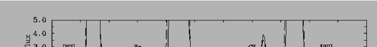
Figure 3: Gaussian fits to nebular lines, showing the nature of the asymmetry at their bases to be of nebular or instrumental origin.

DBS97 noted that the Balmer line shapes of the PN around the two [WC] central stars CPD–56^o8032 and He 2-113 have a broad pedestal. Leuenhagen et al. (1996) determined an upper limit for the stellar hydrogen abundance by fitting this pedestal with synthetic profiles from their non-Local Thermodynamic Equilibrium (non-LTE) code. However DBS97 pointed out that the same broad pedestal was present at the base of forbidden lines which are entirely of nebular origin. This indicates that either a complex nebular velocity field is the cause of the irregular nebular line shapes and of the pedestals at the base of the Balmer lines, or perhaps more likely, that the pedestals observed at the base of these strong lines is due to the grating instrumental profile.

Since the presence of hydrogen in cool [WC] central stars would give a clue about their origin, we have investigated the nebular lines of SwSt 1. In Fig. 3 we present Gaussian fits to H$\alpha$ and H$\beta$, along with other forbidden lines. Although the Balmer lines do present a base which is broader than the Gaussian fit, many other nebular lines, i.e. [N ii] $\lambda$$\lambda$6548,6583 and [O iii] $\lambda$5007, have a similar shape. There is therefore no conclusive evidence for the presence of stellar hydrogen. In Sect. 5.5 we demonstrate how a hydrogen abundance of 10% (by mass) as determined by Leuenhagen and Hamann (1998) is not inconsistent with our own fits.

5.2 Description of the Model Codes

The code adopted to carry out the stellar analysis is the improved Sobolev approximation code isa-Wind (de Koter et al. 1993, 1997). This modelling program solves the radiation transfer equation under the condition of statistical equilibrium in a spherical, extended atmosphere. The line radiation transfer is implemented using an improved version of the Sobolev approximation, which has been shown to be appropriate for the thick atmospheres of Wolf-Rayet stars (de Koter et al. 1997, Crowther et al. 1999 and De Marco et al. 2000).

The wind of SwSt 1, however, is less dense than the winds of most Wolf-Rayet stars, as can be inferred from the overall weakness of its spectral lines. This indicates that the inner, slow moving parts of the stellar atmosphere are exposed in this region, and the Sobolev approximation might break down. To check on the results obtained with isa-Wind, we used the co-moving frame code cmfgen (Hillier & Miller 1998). cmfgen confirmed the results obtained with isa-Wind. However, some of the differences between the two codes are instructive, and although in what follows we refer mostly to isa-Wind, results obtained using cmfgen are presented alongside.

Line blanketing is included in the isa-Wind model by a Monte-Carlo approximation, which includes millions of spectral lines. This is described in detail by Schmutz et al. (1991). Comparison tests have been carried out (Crowther et al. 1999, De Marco et al. 2000) and show the technique to compare reasonably well to a detailed line-blanketing calculation carried out with cmfgen (Hillier & Miller 1998), although the flux shortwards of 400 Å was too hard in the Monte-Carlo technique.

5.2.1 The Model Atom

The number of atomic levels included in the calculation influences the line strengths. Ideally one would want to employ as many lines as possible of as many elements as possible. Unfortunately the larger the atomic model the slower the calculation. As a result a compromise has to be adopted. The atomic model used by our isa-Wind calculation uses Opacity Project data (Seaton 1995) and is summarised in Table 6. The use of super-levels (SL) reduces computational times while at the same time including high-lying levels. Super-levels are groups of levels within which populations are calculated in LTE. The grouping scheme changes for different ions. In Table 6 we indicate the scheme used: “n=4” means that all levels up to and including principal quantum number 4 are included. “sing/trip” means that singlets and triplets are grouped separately; “thr.” indicates that enough super-levels were constructed to include all levels listed in the Opacity Project database up to the ionization threshold. The effect of slight variations in our grouping scheme (as well as the total number of SL) on the synthetic lines was studied for the cases of C ii and C iii and found not to alter the synthetic lines. Only helium, carbon, oxygen, silicon and iron are all included explicitly in the cmfgen calculation, but in somewhat greater detail than in the case of isa-Wind.

Table 6: Summary of the atomic model adopted in our isa-Wind non-LTE simulations of SwSt 1’s stellar wind.

Ion	#	Upper	#	SL Grouping	Dielec-
	Levels	Level	SL		tronic
H i	15	–	–	–	–
He i	19	1P n=4	32	n=20 sing/trip	–
He ii	20	–	–	–	–
C ii	36	2G n=3	2	thr. doub/quart	26
C iii	31	1S n=5	8	thr. sing/trip	31
C iv	9	2F n=4	3	n=7	–
N i	3	2Po n=2	–	–	–
N ii	29	3S n=2	–	–	–
N iii	11	2D n=3	3	n=4 doub/quart	–
N iv	12	1D n=3	–	–	40
N v	14	2D n=6	–	–	–
O i	2	3So n=3	–	–	–
O ii	3	2Po n=2	–	–	–
O iii	41	5So n=3	–	–	–
O iv	11	2D n=3	3	n=4 doub/quart	–
O v	12	1D n=3	–	–	34
Si ii	7	2P n=4	–	–	–
Si iii	16	3Fo n=4	2	n=5 sing/trip	–
Si iv	12	2G n=5	1	n=6	–
S iii	11	3Po n=3	–	–	–
S iv	7	2Se n=4	–	–	–
S v	7	1S n=3	–	–	–
S vi	7	2Fo n=4	–	–	–

5.3 Photon Loss

“Photon loss” is the name given by Schmutz (1997) to the interaction between the photon field of the He ii Ly$\alpha$ line at 303.78 Å and nearby metal lines (e.g. the O iii Bowen lines at 305.72 and 303.65 Å). This can be responsible for a decrease in the ionization equilibrium of the wind with respect to the equilibrium obtained when no such line-line interaction is accounted for. In order to fit the observed spectrum when photon loss is included in the model, the model’s stellar temperature has to be higher, which results in a higher spectroscopic luminosity. This contributes to a lower wind performance number and allowed Schmutz (1997) to calculate a velocity structure for the outer wind of WR6.

De Marco et al. (2000) implemented this approximation in the Sobolev code isa-Wind and showed that results were similar to those obtained using the code cmfgen (for the WC8 stellar component to the $\gamma$ Velorum binary), where line-line interaction is taken into consideration explicitly. Here, we have used the “photon-loss” option, which resulted in only a slightly higher effective temperature ($\sim$2000 K). The effect has been shown by Schmutz (1998) not to be important in the case of O stars, which have weaker winds. This also seems to be the case for the weaker wind of SwSt 1. cmfgen naturally includes line-line interaction and therefore “photon-loss” is automatically taken into account (De Marco et al. 2000).

5.4 Stellar Modelling Technique

Traditionally, modelling of WR stars starts with matching a subset of the observed He i and He ii lines with model line profiles, from which approximate values for the effective temperature and mass-loss rate of the star are determined. The metal abundances are then varied, to afford fits to a representative sample of their lines. Even in modern calculations the velocity law is seldom varied from either a simple or a composite beta-law (e.g. Hamann & Koesterke 2000).

A weakness of this technique is that in a significant number of cases, the choice of diagnostic lines determines what parameters are derived. If excellent fit quality can be obtained for a large number of lines, this gives confidence in the derived parameters, but if only a small subset of the observed lines can be fit by any given model, the parameters are only as good as the choice of diagnostics. Additionally, running non-LTE line-blanketed codes is very time consuming, so that once a reasonable match to a set of lines is achieved, different parameter spaces are seldom explored to determine whether other parameter sets fit the emission lines to a similar degree of accuracy.

The fast calculation speed of the isa-Wind code allowed De Marco et al. (2000) to show that similar synthetic spectra can sometimes be obtained with different combinations of temperature and mass-loss rate. When only a poor fit quality is achieved, or when only a subset of the diagnostic lines is fit simultaneously, it might be hard to choose which model best represents the star, leading to a degeneracy.

The spectrum of SwSt 1 presents a formidable challenge for spectral synthesis, in that it is impossible to fit all the diagnostic lines simultaneously. As a result, it is possible to derive different model parameters depending on which diagnostic lines we decide to include. The exploration of a vast parameter space (stellar temperature, mass-loss rate and metal abundance), made possible by our fast code, together with the use of observational constraints not usually coupled with non-LTE analyses, made it possible to gain a reasonable confidence in our final choice of stellar parameters. Our choice of diagnostic lines comprised all lines included within the levels of our model atom, leaving out those between high-lying levels which might be under-populated. For helium we used He ii $\lambda$4686 ($\lambda$5411 is blended with nebular a [Fe ii] line, and can only be used as an upper limit) and He i $\lambda$5876,4471,6678. As pointed out above, there is extremely little He i in this star, if any, so that the lines (severely blended with nebular components) could only be used to impose an upper limit on the strengths. To constrain the ionization equilibrium one has to appeal to carbon: C ii $\lambda$4267, C iii $\lambda$5696 and $\lambda$8500, and C iv $\lambda$$\lambda$5801,12 and $\lambda$5470 were employed. These lines are also used to determine the carbon abundance. To constrain the oxygen abundance we used O iii $\lambda$5592 (all other lines are too weak or dominated by the nebula).

Once the diagnostic lines were chosen, an approximate value for the temperature and mass-loss rate was obtained, for which reasonable fits were achieved. Since no combination of $T_{*}$, $\dot{M}$ and carbon abundance fitted the spectrum to a satisfactory level, in that the synthetic lines were always too broad in the core and too narrow at the base, we experimented with different velocity laws. In particular we tested velocity laws with progressively slower flows in the inner regions, so as to reduce the line widths, maintaining the observationally-derived value of $v_{\infty}$. The electron density change induced by the different laws changes the wind opacity, with a repercussion on the line ionization equilibrium of the star, and therefore on the line intensities. Consequently different basic parameters are implied by different velocity laws.

5.5 Stellar Model Results

Figure 4: isa-Wind model fits (thick solid line) to the optical and UV stellar rectified spectrum of SwSt 1 (dotted line). The cmfgen models fits (thin solid line) are presented alongside.

Table 7: Stellar parameters from our non-LTE models (isa-Wind and cmfgen), compared with those of Leuenhagen & Hamann (1998; LH98), before and after scaling them to our own adopted distance.

V	E(B–V)	D	MV	T∗	R∗	log(L/	log($\dot{M}$/	v∞	$\eta$	$\beta_{H}$	$\beta_{He}$	$\beta_{C}$	$\beta_{O}$	$\beta_{N}$	Ref.
(mag)	(mag)	(kpc)	(mag)	(kK)	(R⊙)	L⊙)	M⊙ yr-1)	(km/s)		%	%	%	%	%
11.48	0.46	2.0	–1.45	40	2.0	3.95	–6.72	900	0.9	$<$10a	37	51	12	$\sim$0	isa-Wind
11.48	0.48	2.0	–1.51	46	1.5	3.95	–6.84	800	0.6	0	53	32	15	0	cmfgen
11.9	0.41	1.4	–1.10	35	1.0	3.27	–6.90	400	1.3	$<$10	44	53	3	$<$0.5	LH98
–	–	2.0	–1.45	35	1.4	3.49	–6.79	400	1.3	$<$10	44	53	3	$<$0.5	LH98 scaled
a Limit from model profile fitting does not include possibility of blend with nebular emission (see text).

Model fits to the stellar spectrum of SwSt 1 are presented in Fig. 4 (thick and thin solid lines for isa-Wind and cmfgen models, respectively, dotted line for the observations), while the model parameters are presented in Table  7, together with the results of Leuenhagen & Hamann (1998), scaled to our adopted distance. In what follows we discuss the results obtained with the modelling code isa-Wind, followed by a discussion of additional results obtained with the code cmfgen to later.

5.5.1 isa-Wind

He ii $\lambda$4686 is well reproduced, while He ii $\lambda$5411 and He i $\lambda$$\lambda$5876,6678, and other lines which suffer blending with nebular emission, are within reasonable limits. Other synthetic He ii lines (e.g. $\lambda$4542 and $\lambda$4200) are in absorption with wide wings. Since these wings are not observed, and He i lines are mostly of nebular origin, we have have not used these lines as diagnostics.

C iv $\lambda$5801,12 is over-predicted, C iv $\lambda$5470 is well matched, while C iv $\lambda$4441 is somewhat weak. In order to fit C iv $\lambda$$\lambda$5801,12 the effective temperature could not be higher than 35 kK, no matter what other parameters are adopted. However at this temperature the $\lambda$5470 line is in weak absorption. C iv $\lambda$5470 has a better-understood formation mechanism compared to $\lambda$$\lambda$5801,12 (Hillier & Miller 1999, Dessart et al. 2000) and was therefore given priority in the fitting procedure. Additionally, at 35 kK the fit to the C iii $\lambda$4650 line is much worse, with the synthetic line too weak. C iii $\lambda$5696,8500 are also well matched by the model but C ii $\lambda$4267 is poorly matched, with the model line being much too weak. However the C ii $\lambda$$\lambda$6578,6583 blend has a very reasonable fit (C ii $\lambda$$\lambda$7231,7236 is severely affected by telluric absorption and blending with nebular emission line components and was therefore not fitted). The problem with C ii $\lambda$4267 might be linked to insufficient levels in the atomic models. However we have experimented with more levels and included a considerable number of super-levels and dielectronic recombination lines. Since a much stronger synthetic $\lambda$4267 (obtained by lowering the effective temperature) would lead to over-fitting $\lambda$$\lambda$6578,83, we still suspect the model atom is the reason for the problem. If a cooler stellar temperature is used to try and enhance C ii $\lambda$4267, all fits deteriorate, even if the mass-loss rate is reduced to restore the He i/He ii equilibrium. Increasing the mass-loss rate so as to enhance recombination of C iii to C ii, and so increase the strength of the C ii $\lambda$4267 line, also fails. A higher mass-loss rate is also excluded by the fact that by increasing its value by 0.1 dex from the value reported in Table 7, all model lines of C iii acquire deep P-Cygni absorptions, which are not observed. Additionally the He i lines increase in strength, in a way that cannot be compensated for by a larger temperature without losing the C iii/C iv balance.

Increasing the carbon abundance, in steps, from C/He=0.2 to 3 (by number), while adjusting other parameters, does not achieve an improvement in the fits. On the other hand, once the effective temperature and mass-loss rate have been determined, the C/He ratio can be determined with a 50% accuracy. Even with the highest carbon abundance, the C ii line did not increase for the temperature regime which satisfied the other lines. Additionally, when enhancing the C/He ratio the ionization equilibrium of the star is upset in such a way that He ii lines are drastically decreased, which results in having to increase the temperature, at which point other carbon lines do not fit any more, most noticeably C iv $\lambda$$\lambda$5801,12, whose excitation is almost entirely dependent on temperature.

Returning to the C iii line blend at 4650 Å, and to line shapes in general, we have used a velocity law which is slower than $\beta$=1 in the inner parts of the wind (in accordance with that found by Hillier & Miller (1998), Crowther et al. (1999) and De Marco et al. (2000)). For every parameter set, we tested a number of velocity laws with progressively slower winds in the inner parts of the flow. These are shown in Fig. 5. The slower the velocity law, the stronger and narrower the lines become (for identical stellar parameters). As a result each adopted velocity law implied a new set of parameters, resulting in a trend of a somewhat cooler stellar temperature and lower mass-loss rate for slower velocities. For the slower velocity laws, narrower line profiles were accompanied by more redward-displaced P-Cygni absorptions. As a result it was relatively easy to choose the best velocity law from the position of the P-Cygni absorption (as well as the overall line width and shape) of lines such as C iii $\lambda$4650 and C iv $\lambda$$\lambda$5801,12. The velocity law which matched the position of the P-Cygni profiles is marked as a thin solid line in Fig. 5 (left panel) and can be parametrised following the formula of Hillier and Miller (1998) with $v_{\rm ext}$ = 500 km s^-1, $v_{\infty}$ = 900 km s^-1, $\beta_{1}$=1 and $\beta_{2}$=8. This resulted in the best match to the line shapes. In Fig. 5 (right panel) we present profile fits obtained using a $\beta$=1 law, and two slower laws. The model parameters were adjusted in each case to reproduce the line’s peak intensity. As can be seen, the $\beta$=1 law generates profiles which are too broad, while the dot-dash line produces profiles too narrow at the base but too broad in the core.

Figure 5: Left panel: alternative velocity laws compared to a $\beta$=1 law (thick solid line). The adopted law (thin solid line) significantly improved the line fits, making lines broad at the base and narrow in the core, and reproduced the position of their P-Cygni absorptions, while the other laws produced lines which were too broad or too narrow. Right panel: isa-Wind profile fits to C iii $\lambda$5696 (top) and C iv $\lambda$$\lambda$5801,12 (bottom). The dotted line represents the data, the thick solid line represents the model calculated using a $\beta$=1 velocity law, the thin solid line represents the model with the velocity law used for the final model of this paper, and the dashed line shows the slowest velocity law attempted. Model parameters are adjusted to fit the peak intensity of C iv $\lambda$$\lambda$5801,12.

In summary, although the fits presented in Fig. 4 (thick solid line) are not excellent, there is no other parameter combination of mass-loss rate, temperature and C/He number ratio which would satisfy the observed spectrum to a higher degree of accuracy. The derived quantities and their errors are therefore the following: $T_{*}$=(40 000 $\pm$ 2000) K, $\log({\dot{M}}/$M_⊙) = (–6.72 $\pm$ 0.1), C/He = (0.46 $\pm$ 0.20) and O/He = (0.08 $\pm$ 0.02) (by number). The wind performance number $\eta$ (=$L/({\dot{M}}{v_{\infty}}$c) is 0.9, indicating that the wind of SwSt 1 can be driven radiatively in the single scattering limit. The derived stellar luminosity of 8900 L_⊙ is towards the high end for a PN central star (implying a relatively large stellar mass). It is difficult to determine the mass which corresponds to this luminosity since the highest core mass for which Vassiliadis and Wood (1994) calculated Milky Way initial abundance helium-burning tracks was 0.63 M_⊙, but inspection of their Fig. 8 indicates that our derived luminosity for SwSt 1 at 40 000 K is only slightly above the LMC-abundance evolutionary track for a 0.679 M_⊙ core mass.

The helium, carbon and oxygen abundances are 37%, 51% and 12% by mass, respectively, implying a C/O mass ratio of 4.3. The oxygen abundance in particular is obtained from fitting the O iii line at 5592 Å. The lower and upper limits for the O/He ratio allowed by the fit of the $\lambda$5592 line are 9% and 15%. Additional uncertainty derives from fitting a single line. We note that if a lower effective temperature were to be adopted, the oxygen abundance determined by a fit to this O iii line would be higher still.

In Fig. 6 we show the isa-Wind synthetic spectrum, compared with the IR, optical and IUE de-reddened data. A slight over-compensation of the 2200 Å feature by the adopted E(B–V)=0.46 is not considered worrying in view of the known variations in the relative strength of this feature (Mathis 1994), since the overall continuum slope is well matched by our V-scaled synthetic spectrum (if we make an exception for the far blue and red edges of the optical spectrum). By adopting reddening values as low as 0.30 (which nulls the 2200 Å feature) the continuum slope is clearly too gentle to match the model, while for a reddening value of 0.50 the slope will be too steep. In Fig. 6 we also plot the near-IR SOFI spectrum (scaled to the J magnitude of Allen & Glass (1974)) and colour-corrected IRAS photometry values, together with blackbody curves with temperatures 1200 K and 230 K. These curves indicate that some of the dust around this PN is very hot. This is in agreement with the study of Zhang & Kwok (1991).

5.5.2 cmfgen

The fit quality obtained with the code cmfgen is very similar to that obtained with isa-Wind. Although some lines are better reproduced (e.g. C iv $\lambda$$\lambda$5801,12) others are somewhat worse (e.g. C iv $\lambda$4441). The broad He ii absorption lines wings obtained with isa-Wind are somewhat narrower in the models fits of cmfgen, in better agreement with the data. C iii $\lambda$1909 is weaker and more in agreement with the observations (note that in Fig. 4 this line is a blend of stellar and nebular components, as can be appreciated by inspecting Fig. 7). On the other hand the shape of the C iii-iv blend at $\sim$4650 Å is somewhat worse in the cmfgen fits, and the C iii line at 8500 Å has an unobserved P-Cygni absorption. The fit to the only oxygen diagnostic line, i.e. O iii $\lambda$5592, is similar to the one obtained with isa-Wind. The stellar parameters obtained with cmfgen are presented alongside those obtained with isa-Wind in Table 7. Overall, the derived stellar parameters for SwSt1 using CMFGEN match closely with those from ISA-wind, except that the stellar radius is smaller, implying a higher stellar temperature of 46kK. The mass-loss listed in Table 7 does not consider clumping. Almost identical fits can be obtained with a filling factor of 10% with clumping starting at $v=100$ km s^-1. In this case the mass-loss is 7$\times$10^-8M_⊙ yr^-1 or a factor of two lower than obtained without clumping. Due to the relatively low wind density, the electron scattering wings cannot be used to constrain the clumping. The only noticeable changes are in C iii $\lambda$9710 and $\lambda$1909 where clumped models give 20% weaker emission. However, since the latter is dominated by the nebula and the former is only included in our low resolution SOFI data, these cannot provide any useful constraint.

The only considerable difference between the modelling efforts with isa-Wind and cmfgen is that the stellar abundances are discrepant (Table 7). This is possibly due to the different cocktail of atomic data used by the model codes, although, as it is frequent with complex non-LTE codes, it might also be due to a mix of factors hard to trace. In particular the carbon and oxygen mass fractions are 32% and 15%, respectively, compared to isa-Wind’s 51% and 12%. This translates into a C/O mass ratio of 2.1 for cmfgen versus 4.3 for isa-Wind. Both cmfgen and isa-Wind values are higher than solar ($\sim$0.4). The maximum value that the C/O ratio can attain according to the models (Herwig 1999), is the intershell value, $\sim$4. So, although both values are acceptable, the isa-Wind value would imply an extremely effective third dredgeup.

We obtain a good fit of the cmfgen model flux distribution to the dereddened data, although a slightly higher value of the reddening (E(B–V)=0.48 mag) had to be adopted.

5.5.3 Comparison with the Analysis of Leuenhagen & Hamann 1998

Leuenhagen & Hamann (1998) present fits to their 1 Å-resolution optical spectrum that are not dissimilar in quality from our own, although they fit a smaller spectral range. The effective temperature of 40 kK derived with the isa-Wind modelling code, is higher than their 35 kK. Our mass-loss rate is similar to the one derived by Leuenhagen & Hamann (once the different distances are taken into account), while our final wind velocity is more than twice as large. Leuenhagen & Hamann (1998) have not determined $v_{\infty}$ from the C iv line, limiting themselves to fitting the widths of the optical lines. We have already seen how these lines are peculiarly narrow and in apparent disagreement with the value indicated by the P-Cygni absorption of C iv $\lambda$1550. Inspecting their Fig. 3 we notice that their model optical lines are too narrow and suffer from the same problem as our fits with a $\beta$=1 velocity law.

The hydrogen abundance of 10% (by mass) determined by Leuenhagen & Hamann (1998) as an upper limit, when used in our model, produces a synthetic H$\alpha$-He ii line blend which is not entirely in disagreement with our observations. Therefore, based solely on this fit, we confirm their determination. On the other hand, as already noted in Sec. 5.1.1 the blend’s shape might be due to either nebular emission or the instrumental profile, since nebular forbidden lines exhibit the same pedestal. Our isa-Wind carbon abundance is similar to that determined by Leuenhagen & Hamann (1998), while the carbon abundance obtained with cmfgen is lower. Our oxygen abundance, obtained with either of the two codes, is higher than the abundance derived by Leuenhagen & Hamann (1998).

Figure 6: Top panel: the de-reddened ultraviolet (IUE), optical (UCLES) and near-infrared (SOFI) spectra of SwSt 1 (dotted line), compared with the best-fitting isa-Wind stellar model (solid line). Bottom panel: the near-infrared (SOFI) and mid-infrared (ISO SWS) energy distribution of SwSt 1 (dotted line) compared to the flux distribution from the best-fitting isa-Wind stellar model (solid line, $\log$$\lambda$$<$4.4) and 1200 K and 230 K blackbody curves (solid line, $\log$$\lambda$$>$4.4). Ground-based infrared photometry (Allen & Glass 1974; Cohen & Barlow 1974) and colour-corrected IRAS fluxes are also plotted (square symbols). Wavelength units are Å and flux units are ergs cm^-2 s^-1 Å^-1.

6 Nebular Abundance Analysis

6.1 Nebular Line Fluxes

Table 8: Observed (F_λ) and de-reddened (I_λ; E(B–V)=0.46) nebular line intensities for SwSt 1 from the 1993 UCLES spectrum. The de-reddened H$\beta$ flux is 1.50$\times$10^-10 erg cm^-2 s^-1. Errors are gauged at 10%. The lines’ rest wavelengths are from Kaufman and Sugar (1986). The spectral resolution is indicated at the beginning of each Section.

Ion	$\lambda_{o}$	FWHM	Fλ	100$\times$Iλ
	(Å)	(km s-1)	(ergs cm-2 s-1)	/I(H$\beta$)
$\Delta$v$\sim$900 km s-1
C ii]	2326	–	3.9$\times$10-12	97
$\Delta$v$\sim$30 km s-1
C iii]	1906.7	–	5.7$\times$10-13	13
C iii]	1908.7	–	2.0$\times$10-12	38
$\Delta$v$\sim$20 km s-1
$[$O ii]	3726.0	44	6.51$\times$10-12	30.0
$[$O ii]	3728.8	46	2.55$\times$10-12	11.7
$[$Ne iii]	3868.8	40	3.35$\times$10-14	0.48
$[$S ii]	4068.6	41	5.23$\times$10-13	2.2
$[$S ii]	4076.3	41	2.05$\times$10-13	0.85
$\Delta$v$\sim$8 km s-1
H$\delta$	4101.7	44	6.20$\times$10-12	24.7
H$\gamma$	4340.5	41	1.19$\times$10-11	44.9
$[$O iii]	4363.2	31	7.11$\times$10-14	0.27
He i	4471.5	38	6.96$\times$10-13	2.5
H$\beta$	4861.3	41	3.22$\times$10-11	100
$[$O iii]	4958.9	34	3.80$\times$10-12	11.4
$[$O iii]	5006.8	33	1.01$\times$10-11	29.5
$[$Ar iii]	5191.8	33	1.38$\times$10-14	0.04
$[$N i]	5197.9	77	4.80$\times$10-14	0.13
$[$N i]	5200.2	73	2.91$\times$10-14	0.08
$\Delta$v$\sim$20 km s-1
$[$O i]	5577.3	30	7.83$\times$10-14	0.19
$[$N ii]	5754.6	28	1.42$\times$10-12	3.3
He i	5875.7	42	3.17$\times$10-12	7.1
$[$O i]	6300.3	49	7.43$\times$10-13	1.5
$[$S iii]	6312.1	39	1.30$\times$10-12	2.6
$[$O i]	6363	49	2.45$\times$10-13	0.49
$[$N ii]	6548.0	46	1.64$\times$10-11	31.1
He i	6678.1	39	9.26$\times$10-13	1.7
$[$S ii]	6716.5	62	3.91$\times$10-13	0.72
$[$S ii]	6730.8	55	7.92$\times$10-13	1.4
He i	7065.2	39	2.11$\times$10-12	3.6
$[$O ii]	7318.6	–	3.96$\times$10-12:	6.4
$[$O ii]	7319.4	–	4.35$\times$10-11:	70.7
$[$O ii]	7329.6	33	8.36$\times$10-12	13.6
$[$O ii]	7330.7	35	8.62$\times$10-12	14.0
$[$Ar iii]	7751.1	34	7.13$\times$10-13	1.1
$[$S iii]	9531.0	38	7.53$\times$10-11	90.7

The nebular spectrum of SwSt 1 is much stronger and slightly higher in excitation than that of the PN with [WC10] central stars analyzed by DBS97 and De Marco & Crowther (1998). Many nebular He i lines could be measured: amongst them we selected those at 4471.5, 5875.7 and 6678.1 Å, disregarding the line at 7065.2 Å due to its being dominated by collisions and the possibility that it is affected by telluric absorption. The [O ii] line complex at 7325 Å is made up of 4 lines with wavelengths 7318.8, 7319.9, 7329.6, and 7330.6 Å, where the individual components are partly blended. Unfortunately, the blend at 7319 Å was affected by an echelle order join which removed a part of the flux. In order to obtain a measurement of the flux in those lines we therefore snipped the section containing the join. The snipped line, despite missing the central part, still had clearly identifiable wings and could therefore be successfully fitted with a Gaussian. We nonetheless decided to assign a 50% uncertainty to it and did not use it in any of the parameter determinations. The [O ii] lines at 3726.0 and 3728.8 Å are resolved and completely un-blended with any stellar feature. [O iii] lines appear at 4363.2, 4958.9 and 5006.8 Å.

All four [S ii] nebular lines included in our wavelength range could be measured, namely the lines at 4068.6, 4076.3, 6716.5 and 6730.8 Å. The line at 4068.6 Å was found to lie on an order join. However since abundance results obtained with it or with the weaker lines at 4076.3 Å were very similar, we decided to treat it normally and only assign it a marginally higher uncertainty. To determine the abundance of S²⁺, we used $\lambda$9531.0. The telluric water vapour line at 9069.126 Å affects the measurement of the [S iii] line at 9068.9 Å since its measured ratio to the $\lambda$9531 line is 0.28, lower than the theoretical ratio of 0.403.

Three lines of singly ionized nitrogen reside in our spectral range, but as the [N ii] ratio $\lambda$6583/$\lambda$6548 was equal to 1.4, instead of 2.90, we decided that the strong $\lambda$6583 line was saturated (as was H$\alpha$) and did not include it in any of our determinations. Together with the $\lambda$6548 line we used [N ii] $\lambda$5755.

To derive the nebular C/H ratio we used IUE observations of the semi-forbidden C ii] $\lambda$2326 and C iii] $\lambda$1909 lines. We assume the stellar contribution to $\lambda$2326 to be negligible, while we could de-blend the stellar and nebular contributions to C iii $\lambda$$\lambda$1906,1909 using the high resolution IUE spectrum (Fig. 7).

Besides the lines listed in Table LABEL:tab:nebular_fluxes, we identify forbidden lines of Fe⁺ (e.g. [Fe ii] $\lambda$4606), Fe²⁺ (e.g. [Fe iii] $\lambda$4881) and possibly Fe³⁺ (e.g. [Fe iv] $\lambda$5677). We also identify [Ne iii] $\lambda$3868, [Ar iii] $\lambda$5191.8 $\lambda$7135.8 (affected by an order join) and $\lambda$7751.1 and [Cl iii] $\lambda$5517.7 and $\lambda$5537.9. A line list is presented in Appendix B.

Figure 7: The high resolution IUE spectrum of SwSt 1 showing the semi-forbidden stellar-nebular blend of C iii] $\lambda$1906,1909.

6.2 Nebular Temperature, Density and Abundances

Table 9: The nebular electron temperature and density adopted for SwSt 1, along with values from the literature.

Te (K)	log(Ne)	E(B–V)	Ref.
10 500 $\pm$ 500	4.5 $\pm$ 0.2	0.46	this work
11 400 $\pm$ 500	5.0 $\pm$ 0.1	0.41	dFPV87
8000	5.0 $\pm$ 0.1	0.34	FGC84

In Fig. 8 we plot a nebular diagnostic diagram for SwSt 1. From a weighted mean of the diagnostic lines we adopt values for the electron temperature and density of 10 500 K and 31 600 cm^-3 (log(N_e)=4.5), respectively (Table 9).

The temperature implied by the [O iii], [S iii] and [Ar iii] diagnostic ratios is between 11000 K and 10000 K for electron densities between 10³ and 10⁵ cm^-3. The C iii] $\lambda$1909/$\lambda$1906 ratio of 0.34 indicates $\log$$N_{e}$=5.1 for $T_{e}$ in the range 9000–14000 K. However this line ratio is severely affected by the blend with the stellar component. De-blending by fitting nebular and stellar components to the doublet resulted in a large uncertainty.

The diagnostic ratios from singly ionized elements seem to agree on a lower density (4.0$<$log(N_e)$<$4.5), if we make an exception for the [O ii] ratio $\lambda$3727/$\lambda$7330. This ratio uses lines from two different grating settings and therefore might be affected by errors in the flux calibration. However if this were the cause of the discrepancy we would also have to be wary of the [S iii] $\lambda$9531/$\lambda$6312 ratio (which we have used above) and the [S ii] $\lambda$4072/$\lambda$6725 ratios, although these employ the green and red settings and not the blue and red settings used by the [O ii] $\lambda$3727/$\lambda$7330 ratio. The ratios [O ii] $\lambda$3727/3729 and [S ii] $\lambda$6717/6731 are unreliable because they are at their high density limit. Therefore only [S ii] $\lambda$4072/$\lambda$6725 yields a reliable density diagnostic. From [S iii] $\lambda$6312/$\lambda$9531, [O iii] $\lambda$4959/$\lambda$4363, [Ar iii] $\lambda$7751/$\lambda$5192, [N ii] $\lambda$5755/$\lambda$6548 and [S ii] $\lambda$4072/$\lambda$6725 we derive T_e=10 500 K and log(N_e/cm^-1)=4.5.

Although the HST images point to a somewhat stratified PN (with the [O iii] image being smaller than the H$\beta$ one) we feel inclined to average the results obtained from the singly and doubly ionized elements. SwSt 1 is a young and compact PN and we therefore feel unjustified in using different electron density and temperature combinations for the singly and doubly ionized regions, a choice that is more appropriate for more extended, higher ionization objects.

Figure 8: Diagnostic diagram, log(N_e) vs T_e, for SwSt 1. The solid lines are obtained from ratios of ions in the first stage of ionization, the dashed lines are for ions in the second ionization stage.

Flower et al. (1984) also derived log(N_e)=5.0 for SwSt 1 from the high resolution IUE spectrum of the C iii] $\lambda$$\lambda$1907,1909 diagnostic lines. They also quoted an upper limit for the electron density of 2$\times$10⁴ cm^-3, derived from the [O ii] $\lambda$3729/$\lambda$3726 ratio (which is almost identical to ours), however they argued that this ratio is too close to the high density limit to be reliable. Their temperature determination, using the [O iii] $\lambda$5007/$\lambda$4363 ratio, was 8800 K (for E(B–V)=0.70), not inconsistent with our own value (although we employ a lower reddening, the effect is not major over such a short baseline). However their determination using the [O iii] $\lambda$5007/$\lambda$1663 ratio implies a higher electron temperature (15 000 K). If we ascribe the discrepancy to the use of two different spectra in the second determination (IUE and optical), which might have imperfect absolute flux calibrations, we can reconcile our own determinations of the temperature and density for the doubly ionised element with theirs. de Freitas Pacheco and Veliz (1987) derived log(N_e/cm^-3)=5.0 and T_e=(11 400 $\pm$ 500) K, from [S ii] $\lambda$$\lambda$4068,76/$\lambda$$\lambda$6716,31, [O iii] $\lambda$4363/($\lambda$4959+$\lambda$5007) and [N ii] $\lambda$5755/$\lambda$$\lambda$6548,84. Their diagnostic diagram is not inconsistent with our own.

Table 10: Nebular ionic abundances for SwSt 1.

Ratio	Abundance	Lines
		Used
He+/H+	0.044 $\pm$ 0.004	He i $\lambda$$\lambda$4471,5876,
C+/H+	1.21(-4)a $\pm$ 0.60(-4)	C ii]$\lambda$2326
C2+/H+	1.19(-4) $\pm$ 0.24(-4)	C iii]$\lambda$1909
N+/H+	1.99(-5) $\pm$ 0.20(-5)	$[$S ii]$\lambda$$\lambda$5755,6548
O+/H+	2.44(-4) $\pm$ 0.24(-4)	$[$O ii]$\lambda$$\lambda$3726,3729,7330
O2+/H+	1.05(-5) $\pm$ 0.10(-5)	$[$O iii]$\lambda$4959
Ne+/H+	9.77(-5) $\pm$ 1.19(-5)	[Ne ii] 12.8 $\mu$mb
Ne2+/H+	3.94(-6) $\pm$ 0.80(-6)	[Ne iii] $\lambda$3868
S+/H+	2.96(-7) $\pm$ 0.30(-7)	$[$S ii]$\lambda$$\lambda$6713,6731,
S2+/H+	4.23(-6) $\pm$ 0.80(-6)	$[$S iii]$\lambda$9531
a1.21(-4)=1.21$\times$10-4
bline flux from Aitken and Roche 1982

Our derived abundances are listed in Tables 10 and 11, where they are compared with the mean values for Type-I and non Type-I PN from Kingsburgh & Barlow (1994). The quoted errors derive from errors on the flux measurements and do not take into account errors on the electron temperature and density. The C/H number ratio of 2.4$\times$10^-4 is not as high as for CPD-56^o8032 (63$\times$10^-4; DBS97), He 2-113 (50$\times$10^-4; DBS97) or M 4-18 (12$\times$10^-4; De Marco & Crowther 1998) and lower even than the mean PN value as determined by Kingsburgh and Barlow (1994; 5.49$\times$10^-4). Additionally, with C/O=0.94, SwSt 1 qualifies as an O-rich PN Flower et al. (1984) obtained C/O=0.72, while de Freitas Pacheco and Veliz (1987) derived C/O=0.54. The C/O ratio is consistent with the presence of a silicate emission feature at 10 $\mu$m (see Aitken & Roche 1982 and the SWS spectrum plotted in Fig. 6).

To obtain the N/H number ratio we multiplied the N⁺/H⁺ ratio by an ionization correction factor of 1.05, obtained from the ratio of total oxygen to singly ionized oxygen abundances, in accordance with Kingsburgh and Barlow (1994).

7 HST Images

Perek and Kohoutek (1967) quote an optical angular diameter of 5 arcsec, while Aaquist and Kwok (1990) measured a 5 GHz radio diameter of only 1.3 arcsec. No resolved optical image of SwSt 1 was found in the literature. SwSt 1 was observed in 1992 by HST in the H$\beta$ and [O iii] $\lambda$5007 lines, as part of a WF/PC snap–shot survey (two exposures per filter). These four pre-COSTAR images were already calibrated by the pipeline process (details can be found in the HST data handbook). DBS97 used the stellar [O iii] images as a point spread function to de-convolve their images of CPD–56^o8032 and He 2–113. However the nebula around SwSt 1 is more highly ionised than the ones around CPD–56^o8032 and He 2–113, as revealed by the prominent [O iii] lines observed in our spectrum. Hence the [O iii] image could not be used as a point spread function to de-convolve the H${\beta}$ image. We therefore used the program Tiny Tim (V4.0) to create theoretical PSFs for the H$\beta$ and [O iii] images (the theoretical H$\beta$ PSF is shown in Fig. 9 together with the raw images).

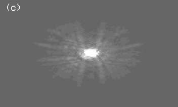
Figure 9: HST images of SwSt 1; a) The average of the two raw H$\beta$ images; b) the average of the two raw [O iii] images; c) the synthetic point spread function generated by the program Tiny Tim; the FOV is 6 arcsec, north is towards the top, east to the left.

Figure 10: De-convolved H$\beta$ (a) and [O iii] (b) HST images of SwSt 1; The images are displayed on a log scale; the FOV is 2.6 arcsec, north is towards the top, east to the left.

The de-convolved images of SwSt 1 (Fig. 10) reveal a broken ring of diameter ((1.3$\times$0.9) $\pm$ 0.2) arcsec, elongated in the east–west direction, in agreement with the radio images of Kwok et al. (1981) and Aaquist and Kwok (1990), but smaller than the 5 arcsec quoted by Perek and Kohoutek (1967). Although the images are of poor quality, this structure could be a ring whose plane is at about 30^o from the line of sight. If we take 1.3 arcsec as the true diameter, a distance of 2.0 kpc and the expansion velocity of 21 km s^-1 would imply a dynamical time-scale of 290 yr for the outer edge of the ionized material (although we do not know how far the neutral shell extends).

The [O iii] image appears smaller than the H$\beta$ image (about 75% of the area), as can be seen from overlaying the normalised contours of the [O iii] image onto the grey–scale plot of the H $\beta$ image (Fig. 11). This is consistent with ionization stratification of the PN. Further confirmation of the stratified structure of this PN comes from analysing the nebular line widths as a function of ionic charge (Fig. 12). After de-convolving the FWHM of individual lines with the respective instrumental profiles, nebular forbidden lines arising from singly ionised ions (e.g. [N ii] $\lambda$6548 and [S ii] $\lambda$6717), as well as lines coming from neutral ions (e.g. [O i] $\lambda$6300) are systematically broader (FWHM$\sim$45–60 km s^-1), while lines arising from doubly ionised ions (e.g. [O iii] $\lambda$5007 and [Ar iii] $\lambda$7750) have widths similar to the Balmer lines (FWHM(H$\beta$)=40.2 km s^-1) or narrower (FWHM$\sim$30–40 km s^-1; see Fig. 12). This is consistent with the lines arising from higher ionization stages being formed in an inner, slower part of the PN, and the lines from lower ionization stages being formed further out in an accelerating part of the flow. The Balmer emission, coming from the entire ionised region, might have been expected to produce broader lines, although it might be more intense in the inner, denser region of the PN, yielding narrower profiles.

Figure 11: De-convolved H$\beta$ HST image of SwSt 1. Over-plotted are the contours from the [O iii] image (Fig. 10).

Figure 12: Comparison of selected nebular lines in the AAT–UCLES spectrum of SwSt 1. The lines are background subtracted and normalised to the peak intensity of the [Ar iii] $\lambda$7750 line.

8 Nebular Modelling

8.1 Zanstra Temperatures

Following the formula of Milne and Aller (1975), for a 5 GHz flux of 243 mJy (the weighted average of Kwok et al. 1981, Milne and Aller 1982 and Aaquist and Kwok 1990, see Section 3.3), we predict an intrinsic H$\beta$ flux of 8.07$\times$10^-11 ergs cm^-2 s^-1. This H$\beta$ flux agrees within the uncertainties with the fluxes of Flower et al. (1984) for their adopted reddening of c(H$\beta$)=0.68. From these de-reddened H$\beta$ fluxes and the distance of 2.0 kpc for SwSt 1 we derive a flux of hydrogen–ionizing photons for the star corresponding to log(Q_o(s^-1))=46.90.

We carried out a Zanstra analysis using blackbody as well as Kurucz ATLAS9 (Kurucz 1991) model atmospheres with log(g)=4.0, the minimum gravity tabulated for atmospheres of the required effective temperatures. We derive a blackbody H i Zanstra temperature of (30 300 $\pm$ 500) K, while the ATLAS9 model grid yields an effective temperature of (34 000 $\pm$ 500) K. The radius predicted for the scaled blackbody is 2.7 R_⊙ at the adopted distance of 2.0 kpc, from which a luminosity of 3550 L_⊙ can be derived. A similar exercise for the Kurucz atmospheres yields a radius of 2.3 R_⊙ and a stellar luminosity of 6300 L_⊙.

de Freitas Pacheco and Veliz (1987) derived a blackbody H i Zanstra temperature of 32 000 K. A comparison by Flower et al. (1987) of the stellar ultraviolet and nebular free–free radio continuum fluxes yielded a blackbody H i Zanstra temperature of 36 000 K, although they found that a 30 000 K blackbody better fitted their optical and UV de-reddened stellar energy distribution.

Table 11: Empirical and modelled nebular abundances for SwSt 1 compared with mean values for Type-I and non Type-I PN from Kingsburgh & Barlow (1994).

Ratio	Abundance	Abundance	Abundance	Abundance
	Empirical	Modelb	Type-I	non Type-I
He+/H+	0.044 $\pm$0.004	0.04	0.129 $\pm$ 0.037	0.112 $\pm$ 0.015
$\log$(C/H)+12	8.38 $\pm$ 0.25	8.40	8.48 $\pm$ 0.30	8.81 $\pm$ 0.30
$\log(N/H)$+12	7.32a $\pm$ 0.10	7.99	8.72 $\pm$ 0.15	8.14 $\pm$ 0.20
$\log$(O/H)+12	8.41 $\pm$ 0.20	8.15	8.65 $\pm$ 0.15	8.69 $\pm$ 0.15
$\log$(Ne/H)+12	8.01 $\pm$ 0.07	7.88	8.09 $\pm$ 0.15	8.10 $\pm$ 0.15
$\log$(S/H)+12	6.65 $\pm$ 0.10	6.62	6.91 $\pm$ 0.30	6.91 $\pm$ 0.30
C/O	0.94	1.79	0.68	1.32
N/O	0.08	0.08	1.17	0.28
aICF(N)=O/O+=1.05, N/H=IFC(N)$\times$N+/H+, following Kingsburgh & Barlow 1994
bAbundances derived from the photoionization model, using the isa-Wind WR
stellar atmosphere as input (Table 12).

8.2 Modelling Strategy and Results

Photo-ionization modelling of PN is the best way to test the internal consistency of an empirical analysis. The Harrington photo-ionization code applied here (Harrington et al. 1982) assumes that the nebula can be represented by a hollow spherical shell which is ionised only by a central star, and sampled by 60 radial grid points.

The Kurucz model and blackbody luminosities and the distance were fixed at the values derived above. An inner nebular angular radius of 0.22 arcsec (approximately 5 pixels) was determined from the HST observations, and scaled to the adopted distance (2.0 kpc) to yield an inner radius of 0.0086 pc. The clumping and vacuum filling factors were varied so as to reproduce the de-reddened H$\beta$ flux. The electron density was kept constant throughout the PN, fixed at the empirically derived value, except in the case of the WR flux distribution, for which this value overestimated the H$\beta$ flux even for extremely low values of the filling factor, a fact that was judged non-physical. In theory, such a high density PN is likely to be optically thick, such that a correct modelling procedure should make sure that the model reaches far enough to include the edge of the Strömgren sphere. This is achieved by increasing the thickness of the PN shell until the the PN recombines at the outer grid points. On the other hand, following this procedure would mean that the thickness of the ionized shell and the corresponding H$\beta$ flux would be much larger than observed, a fact that cannot be compensated for by reducing the filling factor within sensible limits. We therefore used the observed values for the inner and outer radii and accepted an optically thin PN. A non-constant density profile was not attempted. The efforts of De Marco & Crwother (1999) on the PN M4-18 did not produce better results when a variable density profile was adopted. Additionally, for the compact PN SwSt 1 the lack of a high signal-to-noise ratio image means that the density profile cannot be constrained.

As a starting point we adopted the empirically derived abundances. Lines of oxygen and carbon were then fitted by changing their abundances. Carbon and oxygen are important coolants and changing the abundances not only varies the line strengths, but also the nebular electron temperature. When a compromise was reached on the strength of these lines and the electron temperature, lines of sulphur, nitrogen and neon were fitted by varying their abundances. The abundances of other unobserved species were left at the mean PN value as determined by Kingsburgh and Barlow (1994) for a set of 80 southern PN, or at their solar values. When the ionization balance of the element in question is very different from the observations it is arbitrary to decide which lines should be fitted and which should be ignored. In the case of sulphur, we used the strong [S iii] line at 9532 Å, ignoring [S ii] lines. For oxygen, we fitted a compromise of the [O ii] lines $\lambda$$\lambda$3726,29 and $\lambda$7325, forsaking [O iii] lines. For neon, the [Ne ii] line at 12.8 $\mu$m was used, while for carbon a compromise between the C ii] $\lambda$2326 and C iii] $\lambda$1908 lines was used. We note however that because none of the stellar flux distributions reproduces the observations to an acceptable precision, we found it unnecessary to fit individual spectral line fluxes to high accuracy.

Table 12: Comparison of results from photo-ionization models for SwSt 1 with observations (I(H$\beta$)=100), using isa-Wind non-LTE, blackbody and Kurucz plane–parallel energy distributions.

Parameter	Observed	WR	Blackbody	Kurucz
$T_{\em eff}$(K)	–	40.0	30.3	34.0
log($L/L_{\odot})$	–	3.94	3.74	3.80
R(R⊙)	–	2.0	2.7	2.3
log $Q_{0}$(s-1)	46.90	47.53	46.90	46.90
log(I(H$\beta$))	–10.1	–10.1	–10.1	–10.1
Ne(cm${}^{-3})$	31620	15000	31620	31620
$\epsilon$	–	0.76	0.15	0.18
Rinner(pc)	0.0086	0.0086	0.0086	0.0086
Router(pc)	0.0252	0.0252	0.0252	0.0252
MPN(M⊙)	–	0.021	0.009	0.015
$\tau$(H i)	–	0.69	1.3	2.2
He/H	0.04	0.04	0.064	0.15
C/H$\times$104	2.51	2.51	4.68	2.51
N/H$\times$105	1.99	9.86	4.11	2.13
O/H$\times$104	2.57	1.40	1.90	0.78
S/H$\times$106	4.17	4.00	6.00	4.60
Ne/H$\times$105	9.80	7.60	8.80	7.90
1909 C iii]	71	68	33	14
2326 C ii]	85	19	76	208
3726 [O ii]	30	57	39	38
3729 [O ii]	18	23	14	14
3868 [Ne iii]	0.5	0.0	4.8	0.06
4068 [S ii]	2.2	2.5	2.5	3.7
4076 [S ii]	0.85	0.27	0.82	1.2
4363 [O iii]	0.3	0.09	0.4	0.02
4471 He i	2.5	2.3	3.3	1.2
5007 [O iii]	29	204	62	2.2
5755 [N ii]	3.2	2.2	1.9	3.1
5876 He i	7.1	6.7	9.2	3.6
6300 [O i]	1.5	0.0	0.06	0.07
6363 [O i]	0.5	0.0	0.02	0.02
6548 [N ii]	31	30	27	32
6678 He i	1.7	1.8	2.5	1.0
6717 [S ii]	0.7	0.2	0.8	1.1
6731 [S ii]	1.4	0.4	1.9	2.5
7325 [O ii]	28	18	20	23
9532 [S iii]	91	84	92	94
128 000 [Ne ii]	68	67	65	67
C2+/C+	0.98	9.8	0.23	0.17
O2+/O+	0.043	0.81	0.18	0.088
S2+/S+	14	9.7	10.7	15
Ne2+/Ne+	0.040	–	0.063	0.004
$T_{e}$(N+)(K)	10 500	10 500	9300	10 800

In Table 12 we compare the abundances determined from modelling with the empirical values, as well as the predicted line fluxes with the de-reddened observations. None of the stellar atmospheres used reproduces the observed characteristics of SwSt 1’s PN to an acceptable degree of accuracy. In the case of the WR flux distribution, we decided that lowering the electron density to about half the observed value was preferable to having an extremely low filling factor ($\sim$0.02, too low even if the PN is actually a ring as the HST image might suggest). With this value of the electron density, a more acceptable filling factor of 0.76 was needed to reproduce the H$\beta$ flux. However, this implies an optically thin PN. The overall ionization balance is overestimated except that of sulphur, which is underestimated. Interestingly, a cooler WR stellar atmosphere, also failed to reproduce the ionization balance. We tried to use the 35kK model which reproduces most of the stellar spectral features except the C iv/Ciii ionization balance (see Sect. 5.5). This model severely underestimates the nebular ionization balance, while at the same time having a similar problem with the H$\beta$ flux and the filling factor, as outlined above. We therefore believe that the failure of the PN model is not due to the hot WR atmosphere.

The blackbody and Kurucz stellar flux distributions underestimate the ionization balance of carbon, but overestimate that of oxygen. They give mixed results in the case of neon and sulphur. With particular reference to oxygen, we point out that the [O iii] lines used are extremely susceptible to small temperature changes, in particular it appears that for central star effective temperatures above $\sim$38kK the [O iii] lines increase dramatically in flux (Miriam Peña, priv. comm.). For these stellar flux distributions we were able to use the electron density determined from observations, although, once again, we had to accept an optically thin PN, so as to obtain a sensible value for the filling factor. An optically thin PN is however more in disagreement with an electron density of 31 600 cm^-3. The three stellar atmospheres are compared in Fig. 13.

The nebular mass implied by all the stellar flux distributions is very low compared to the canonical value of 0.3 M_⊙ for optically thin PN. As for the optical depth properties of this PN, it is unusual to have an optically thin PN with an electron density as high as we encountered. On the other hand the fact that the Zanstra analysis returns values of the effective temperature lower than determined with an ad hoc modelling of the stellar spectrum with a non-LTE code, might suggest that the H$\beta$ flux is not representative of the hard photon population, i.e. that the PN is indeed optically thin.

In conclusion, no matter the method chosen for the modelling effort, we have found no way of fitting the observed properties of this PN to a satisfactory accuracy. We take this to mean that the modelling tool being used is inadequate for the PN of SwSt 1. In particular the simple shell geometry might be far from the truth of this young PN. Nebular modelling with our cmfgen models atmosphere as input was not attempted. Overall the two flux distributions compare reasonably well, with isa-Wind harder far UV flux being compensated by cmfgen’s higher effective temperature. cmfgen would therefore not succeed in reproducing the [Oiii] lines.

Figure 13: A comparison of the isa-Wind line-blanketed non-LTE model atmosphere (dotted line) with the 30 300 K blackbody flux distribution (dashed line), and a 34 000 K, log(g)=4.0 plane–parallel Kurucz model atmosphere (thick solid line). The H i and He i and other important ionization edges are marked.

9 SwSt 1 between 1895 and 1993

The warm oxygen-rich dust revealed by the 10 $\mu$m silicate emission feature, and the high nebular density, indicate that SwSt 1 has recently made the transition from the AGB. This could indicate that the pulse that caused SwSt 1 to become H-deficient might have occurred in the last century, i.e. after it was first observed in 1895. Since variability of the stellar and nebular lines has been noted by Carlson & Henize (1997) and by de Freitas Pacheco & Veliz (1987), we decided to investigate the variability issue. Photographic spectra of SwSt1 were examined by taking a cut through a scan of the plate that appeared in the original paper. We then applied a rough wavelength calibration. Obviously, some fidelity is lost in this process but the spectra are still useful qualitatively.

SwSt 1 was discovered to be an emission line star by James E. Keeler in 1895 (Fleming 1895). He reported Balmer lines in emission and compared the spectrum to that of $\eta$ Car. Although we could not find his spectrum in the literature, we examined a scan from another plate taken in 1896 which shows only 3 emission lines (H$\beta$ and [O iii] $\lambda$$\lambda$4959,5007) superimposed on a stellar continuum. On the basis of this spectrum, SwSt 1 is referred to as P-Cygni class by Fleming in her log-book. Cannon (1916), referring to these or similar spectra, also assigned SwSt 1 to the P-Cygni class. These early spectra of SwSt 1 are very low dispersion prism spectra. Although P-Cygni profiles had already been recognized in other stars, it is doubtful that they could be resolved on these plates. It is more likely that SwSt 1 was classified as P-Cygni on the basis of bright Balmer lines on top of a stellar continuum. Cannon (1921) mentions the presence of [O iii] $\lambda$$\lambda$ 4959,5007 emission in SwSt 1. She notes that these lines are associated with gaseous nebulae (even though they weren’t identified until 1928).

Subsequently, SwSt 1 was observed spectroscopically on six distinct occasions: by Payne Gaposchkin (1938, source spectra unknown); in 1940 by Swings & Struve (1940; in the range 3600–6680 Å at dispersions of 100 and 50 Å/mm); in 1942 by Swings & Struve (1943; 3600-5300 Å); in 1962 by Carlson and Henize (1979; in the range 3700–6600 Å at a dispersion of 177 Å/mm blue–ward of 5000 Å and 94 Å/mm red–ward of 5000 Å); by Aller (1977, although the date of the spectrum is not indicated; the range of the observations is 5000-8500 Å); in 1976 by Flower et al. (1984; in the range 4260-6710 Å at a resolution of 7 Å); in 1985 by de Freitas Pacheco and Feliz (1987; in the range 3600–6930 Å at resolutions of 6.5 and 0.5 Å); in by Leuenhagen & Hamann (1998; in the range 3800–5000 Å and 5800-6700 Å at a resolution of 1 Å) and by us in 1993 (in the range 3700–5400 Å at a resolution of 0.15 Å and in the range 5400–9200 Å at a resolution of 0.35 Å).

Two trends since 1940 have been suggested in the literature: a weakening of the stellar wind lines and an increasing degree of ionization of both the stellar wind and the PN. The former trend was pointed out by Carlson and Henize (1979), who noted the possible disappearance of several weak stellar O iii and C iii lines between 1940 and 1962, along with the appearance of [Fe ii] and [Fe iii] lines. They also reported the diminution of P–Cygni profiles, from a total of 10 lines (as counted by Swings & Struve, (1940)) to 4 lines, finally concluding that the wind’s density and mass-loss rate must have decreased between the two observations.

We looked at the plate reproductions in the original 1940 and 1962 papers and we also took a cut along the spectral direction of scanned-in versions. To within the precision allowed by our method, we notice no obvious change. It is possible that weak P-Cygni profiles were apparent to Swings & Struve in the original plate material and that these features had become weaker by 1962 when observed by Carlson & Henize. One might in fact expect the star to have gradually lost its hydrogen during its early post-AGB phase. We have no reason to doubt the claim by Swings and Struve that H$\gamma$ and H$\epsilon$ had P-Cygni profiles but not H$\alpha$, H$\beta$ or H$\delta$. However, we would like to point out that H$\alpha$ is generally the first line to develop an emission component and a P-Cygni profile in the presence of a wind. Looking at the 1940 spectrum we do notice however that the stellar continuum is extremely irregular, while in 1960 it is much smoother. Such irregularity, combined with a variety of emission lines could have given the impression of troughs, which could in turn have been interpreted as P-Cygni.

The claim of Carlson & Henize (1979) that [Fe ii] and [Fe iii] emission appeared sometime between 1940 and 1962 is also somewhat suspect, since [Fe ii] emission was already reported previous to 1940, by Payne Gaposchkin in 1938. However by far the most misleading statement about variability reported in the literature is the claim of Carlson and Henize (1979) that the C iii $\lambda$5696 and C iv $\lambda$$\lambda$5801,12 lines are absent from the 1962 spectrum of SwSt 1. These lines are prominent in the spectrum of Swings & Struve (1942) and also in our own spectrum. The Carlson & Henize (1979) 1962 spectrum longward of 5000 Å comes from a very weakly exposed plate compared to their other material. On that plate only the strong nebular [N ii] $\lambda$6583 line and H$\alpha$ are visible, with He i $\lambda$5876 described as being barely visible. The C iii $\lambda$5696 and C iv $\lambda$$\lambda$5801,12 lines are several times weaker than $\lambda$5876 in our spectrum and would be well below their plate limit. On this basis, the claim that C iii $\lambda$5696 and C iv $\lambda$$\lambda$5801,12 are not present in 1962 can be dismissed.

The only spectral change which seems real, comes from the spectroscopy of Aller (1977). From his Figure 4 we see that C iv $\lambda$5470 is much stronger and broader than the neighbouring He ii/[Fe iii] blend at 5411 Å. In the spectrum presented here, the strength of the two lines is comparable. However the C iv lines at 5801 and 5812 Å are not stronger in the Aller spectrum, so that no consistent trend is noticed.

de Freitas Pacheco & Veliz (1987) advocate a second trend, increasing ionization of both the stellar wind and the PN. They were not able to see any nebular [Fe ii] lines in their spectra despite the far superior resolution of their data to earlier spectra, and noticed instead weak lines which they attributed to [Fe iv]. Although de Freitas Pacheco and Veliz do not show any of the spectral regions containing [Fe ii] lines, from the quality of their published spectroscopy we suggest that they would not have been able to observe the weak [Fe ii] lines detectable in our 1993 spectrum. However, since the 1938 and 1962 spectroscopy is likely to have been of poorer S/N than their 1985 data, we conclude that [Fe ii] lines have indeed weakened and that the fact that we do observe them in the 1993 spectrum is only because of our higher resolution. Based on the weakening of the nebular [Fe ii] lines, we conclude that the PN might have increased its level of ionization, although we attach a large uncertainty to this statement. However, the argument that the stellar wind has increased in ionization is based on the erroneous claim by Carlson and Henize (1979) of the absence of the C iv lines at 5801 and 5812 Å in 1962.

In conclusion the arguments for a significant evolution of the spectrum of SwSt 1 in the last century are weak. The PN might have increased its level of ionization slightly, and there might have been some variability in the stellar wind spectrum, but nothing major has happened to this central star in the last 60 years and possibly in the 110 years since it was first observed.

10 Discussion

From the properties derived for SwSt 1 we can state the following. Although the possible distance range of 2–4 kpc is large, even at a distance of 2 kpc the stellar luminosity implied by the models points to a central star mass at the high end of the PN distribution. As we have seen, the distance issue poses a significant obstacle and does not allow us to determine the the stellar and nebular parameters with sufficient accuracy to establish relationships between different objects. Better parallaxes, or expansion distances are the only way to get around the problem. Another way would be to find [WCL] stars in the Magellanic Clouds and use those to characterize the sample. A wide field survey would be needed, sensitive enough to detect emission line stars with equivalent widths of the order of a few Ångstroms and for 8 m-class telescope follow up spectroscopy.

The stellar analysis indicates a hotter star than previously implied (Leuenhagen & Hamann 1998), and more in conformity with the [WC9] spectral classification. The weakness of SwSt 1’s stellar lines can be attributed to a relatively low mass-loss rate, although the derived value of 1.90 $\times$ 10^-7 M_⊙ yr^-1 should be quoted with care because of its distance dependence. Also noteworthy is the stellar wind oxygen abundance. This determination is reliant on a single line of O iii, but no other lines exist in the available spectral range which contradict this determination. The new stellar evolutionary calculations of Herwig (2000) show that the oxygen abundance of models which account for convective overshoot (which begin to account for the severe hydrogen deficiency of WR central stars) should have a 10-20% oxygen mass fraction. This is in agreement with our oxygen determination. Additionally the C/O mass ratio is in the range 2-4 (depending on what modelling effort we rely on), showing third dredge-up enrichment. This is not dissimilar from the values obtained for the [WC10] stars CPD–56^o8032 and He 2-113 of 3.7 and 4.1, respectively.

The PN of SwSt 1 is compact and of high density. It is likely to be stratified as indicated by the HST H$\beta$ image being larger than the [O iii] image and by the lines from higher ionization stages being narrower. The nitrogen abundance is not particularly high, which is surprising if the central star is as massive as is implied by other parameters. Its other nebular abundances are not particularly unusual when compared to the mean values obtained by Kingsburgh and Barlow (1994) for non-Type I PN. We confirm again that the C/O ratio is smaller than unity (0.7 by mass), indicating an O-rich PN. This is interesting in view of the stellar C/O ratio of 2-4, indicating active dredge up between when the nebular material was ejected the present time. A study of the C/O variation as a function of distance from the star is underway for SwSt 1, CPD–56^o5682 and He 2-113 (De Marco et al. in preparation).

The PN neutral envelope presents a fair amount of atomic (e.g. sodium; Dinerstein et al. 1995) and only weak molecular H₂ emission is observed in our SOFI spectrum. We find that modelling this PN with a simple shell geometry and a smooth electron density fails no matter what stellar flux distribution is used. For a distance of 2 kpc, our best fitting model has a luminosity of 8900 L_⊙, significantly higher than the re-radiated IR dust luminosity of 1450 L_⊙, implying that either the dust shell does not absorb and re-radiate the stellar luminosity, or else that our stellar model is not valid. On this line we also note that the relatively low N/H PN abundance ratio does not point to a particularly massive central star. Additionally, if wind strength correlates with luminosity, as is the case for radiationally driven winds, the weakness of the wind would also tend to point to a lower mass.

After carefully assessing the spectral variability reported in the literature by going back to the original publications and spectral plates, we cannot fully corroborate any of the changes reported in the spectrum of SwSt 1. From this we conclude that the star has not changed significantly over the past 100 years. Certainly we have not caught SwSt 1 before the pulse that transformed it into a hydrogen deficient star. The dynamical time-scale of 150–330 yr refers to the edge of the ionized PN, although for such a high density object, we might expect this to be only a lower limit, since the PN material might not be fully ionized.

Appendix A The neutral envelope of SwSt 1

The Na i D lines in the spectrum of SwSt 1 shown in Fig. 1 indicate a complex neutral envelope structure. Below we study this complex line system and compare our findings to those of Dinerstein et al. (1995).

The Na i D line negative LSR radial velocity troughs in the spectrum of SwSt 1 are unlikely to be of interstellar origin since the Galactic radial velocity curve in the direction of SwSt 1 is positive (Fig. 1c). It is therefore likely that these components arise from a neutral envelope enclosing the ionized PN. As such they can be a good tracer of velocity components. We identified two components per line, with radial velocities at (–78 $\pm$ 5) km s^-1 and (–38 $\pm$ 2) km s^-1 (Fig. 1b). If corrected for the heliocentric radial velocity of the nebula, the Na i D line emission components lie at (0 $\pm$ 4) km s^-1, while the two troughs are measured to be at (–70 $\pm$ 5) and (–28 $\pm$ 2) km s^-1. The nebular expansion velocity determined in Section 3.2 is (20 $\pm$ 1) km s^-1. Hence we would expect absorption components of the Na D lines associated with the ionized nebula to be found at a heliocentric radial velocity of about –20 km s^-1. The trough associated with the first component is at about –28 km s^-1, 8 km s^-1 more negative than expected, although this discrepancy can be almost justified by the relative uncertainties. The component at –70 km s^-1 then has to be explained by assuming that SwSt 1’s PN has a neutral velocity component moving at a higher velocity than the ionised ‘shell’ measured by the Balmer lines. For the [WC10] stars CPD–56^o8032 and He 2–113 (DBS97) there is a correspondence between the high velocity components of the Na i D line troughs and the shape of the emission lines of [O i]. The same comparison in SwSt 1 reveals that fitting the [O i] lines with two Gaussians (of which one is forced to have a FWHM=40 km s^-1) cannot encompass components with FWHM larger than 60 km s^-1. This could explain a Na i D line component at about –30 km s^-1 (like the observed component at –28 km s^-1) but not the trough observed at –70 km s^-1. In conclusion, the absorbing sodium must be associated with a different part of the nebula from the collisionally excited neutral oxygen.

Dinerstein et al. (1995) also found evidence for circumstellar sodium around SwSt 1. They measured the emission component of the Na D lines to be at –7 km s^-1, while they determined the absorption component to be at –27 km s^-1 (where their measurements were corrected for a heliocentric nebular radial velocity of –20 km s^-1). These correspond within the uncertainties to our emission component at 0 km s^-1 and absorption component at –28 km s^-1. They did not find a double absorption as we do, and indeed their Fig. 2 is significantly different from our Fig. 1 (a), although their claimed resolution (0.20 Å) is similar to our own. It is not possible at present to resolve this discrepancy. However they did mention the possibility of the existence of higher velocity components in the PN envelope and they compared this effect to the fast low ionization outflows (FLIERs) described by Balick et al. (1993) and Balick (1994).

Appendix B The optical and near-IR spectra of SwSt 1

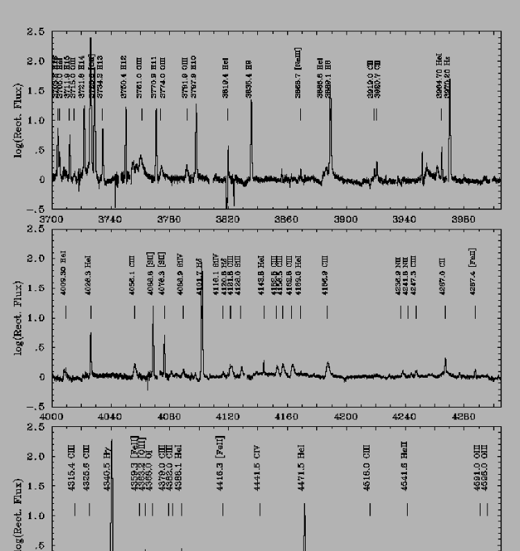
Figure 14: The AAT spectrum of SwSt 1 between 3700 and 4605 Å.

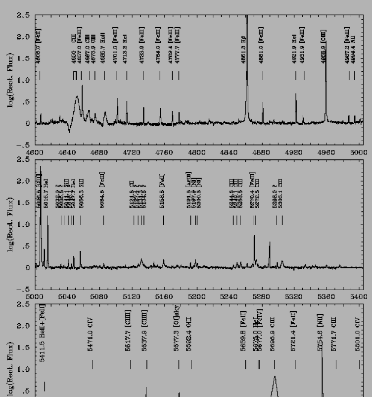
Figure 15: The AAT spectrum of SwSt 1 between 4600 and 5805 Å.

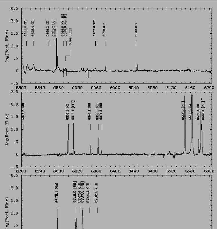
Figure 16: The AAT spectrum of SwSt 1 between 5800 and 7005 Å.

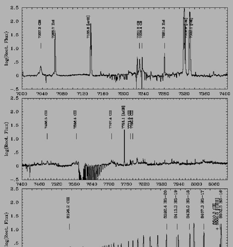
Figure 17: The AAT spectrum of SwSt 1 between 7000 and 8515 Å.

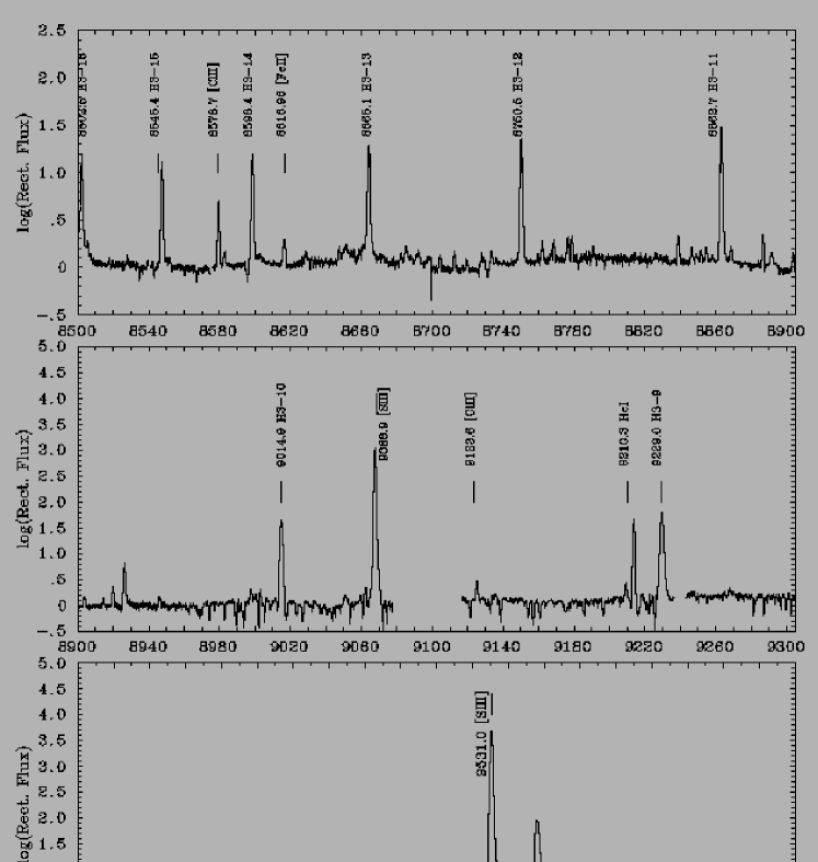
Figure 18: The AAT spectrum of SwSt 1 between 8500 and 9700 Å.

In this Appendix we present the UCL Echelle spectrum of SwSt 1 obtained at the Anglo–Australian Telescope in May 1993 (Figs. 14-18) as well as our near-IR NTT SOFI spectrum (Fig. 19; details of the data acquisition and reduction are presented in Section 2). Due to the strength of the nebular lines compared to the stellar lines, we present the rectified optical spectrum on a log scale.

In Table LABEL:tab:atlas we present a list of the lines we identified in the optical spectrum of SwSt 1. In Column 4 we indicate the origin of the line (s for stellar, n for nebular, is for interstellar), while in Column 5 we list the initials of the authors who have identified those lines in the past. A discussion of the stellar and nebular components of SwSt 1’s optical spectrum has been presented in Secs. 5.1 and 6.1.

The near-IR SOFI spectrum is dominated by strong nebular emission lines of H i (e.g. P$\beta$, Br$\gamma$) and He i (1.083$\mu$m, 2.058$\mu$m), plus [S iii] 9530Å. As reported in Sec. 2.1, we have detected $H_{2}$ (at 2.1218$\mu$m ($v$=1–0, S(1)) for the first time from this young PN.

Table 13: Lines identified in the spectrum of SwSt 1 between 3700 and 9700 Å.

Ion	Wavelength	Multiplet	Origin	Comments
	(Å)	No.
H16	3703.8		n	SS,CH
He i	3705.0	25	n	CH
H15	3711.9		n	SS,CH
O iii	3715.0	14	s	SS
H14	3721.8		n	SS,CH,dFV
$[$O ii]	3726.2	1F	n	SS,CH,dFV
$[$O ii]	3728.9	1F	n	SS,CH,dFV
H13	3734.2		n	SS,CH
H12	3750.4		n	SS,CH
O iii	3761.0	30	s	SS
H11	3770.9		n	SS,CH,dFV
O iii	3774.0	2	s
O iii	3791.3	2	s
O iii	3791.9	2	s	SS
H10	3797.9		n	SS,CH,dFV
He i	3819.4	22	n	SS,CH
H9	3835.4		n	SS,CH,dFV
$[$Ne iii]	3967.7		n
He i	3888.7	2	n	SS
H8	3889.1		n	SS,CH,dFV
C ii	3919.0	4	n	CH
C ii	3920.7	4	n	CH
He i	3964.7	5	n	SS,CH
H$\epsilon$	3970.2		n	SS,CH,dFV
He i	4009.4	55	n
He i	4026.3	18	n	SS,CH
C iii	4056.1	24	s	SS,CH
$[$S ii]	4068.6	1F	n	SS,CH,dFV
$[$S ii]	4076.3	1F	n	SS,CH,dFV
H$\delta$	4101.7		n	SS,CH,dFV
He i	4120.8	16	n
C iii	4121.8	17	s
Si ii	4128.0	3	s	CH
Si ii	4130.9	3	s
N ii	4136.9		s/n?
He i	4143.8	53	n	SS,CH
C iii	4152.5	21	s
C iii	4156.5	21	s	SS
C iii	4162.8	21	s
He i	4169.0	52	n
C iii	4186.9	18	s	SS,CH
N ii	4241.8		s/n?
C iii	4247.3	11	s
C ii	4267.0	6	n+s	CH,dFV
$[$Fe ii]	4287.4	7F	n	CH
C iii	4315.4	48	s
C iii	4325.6	7	s	CH
H$\gamma$	4340.5		n	SS,CH,dFV
$[$Fe ii]	4359.3	7F	n	CH
$[$O iii]	4363.2	2F	n	SS,CH,dFV
O i	4368.0		n	dFV
C iii	4379.0	14	s
C iii	4382.0	14	s
He i	4388.1	51	n	SS,dFV,CH
$[$Fe ii]	4416.3	6F	n	CH

Ion	Wavelength	Multiplet	Origin	Comments
	(Å)	No.
C iv	4441.5		s
C iii	4650.3	1	s	SS,CH
C iii	4651.5	1	s	SS,CH
$[$Fe iii]	4657.0	3F	n	dFV,CH
C iii	4663.6	5	s
C iii	4667.0	5	s	SS
C iii	4673.9	5	s
He ii	4685.7	3-4	s	SS,CH
$[$Fe iii]	4701.0	3F	n	CH,dFV
He i	4713.2	12	n	CH,dFV
$[$Fe iii]	4733.9	3F	n	CH,dFV
$[$Fe iii]	4754.0	3F	n	dFV
$[$Fe iii]	4769.4	3F	n
$[$Fe iii]	4777.7	3F	n
H$\beta$	4861.3		n	SS,CH,dFV
$[$Fe iii]	4881.0	2F	n
He i	4921.9	48	n	CH,dFV
$[$Fe iii]	4930.5	1F	n
$[$O iii]	4958.9	1F	n	SS,CH,dFV
$[$Fe iii]	4987.3		n
N ii]	4994.4		s/n
$[$O iii]	5006.8	1F	n	SS,CH,dFV
He i	5015.7	4	n	dFV
?	5032.0
?	5035.8
?	5041.1
He i	5047.7	47	n
Si ii	5056.0	5	n?
$[$Fe iii]	5084.8
C ii	5121.8
?	5130.8		s
$[$Fe ii]	5158.8	19F	n
$[$Ar iii]	5191.8	3F	n
$[$N i]	5197.9	1F	n
$[$N i]	5200.3	1F	n
C iii	5244.6	4	s
C iii	5249.1	23	s
C iii	5253.5	4	s
$[$Fe iii]	5270.0	1F	n	dFV
C iii	5272.5	4	s
?	5298.0
C iii	5305.1	46	s
He ii	5411.5	4-7	s
C iv	5471.0		s
$[$Cl iii]	5517.7	1F	n	dFV
$[$Cl iii]	5537.9	1F	n	dFV
$[$O i]	5577.3	3F	n	sky
OIII	5592.4	5	s
$[$Fe ii]	5659.8		n
He i	5675.0	?	n
C iii	5695.9	12	s	SS
$[$Fe ii]	5721.4	33F	n
$[$N ii]	5754.6	3F	n	SS,dFV
C iii	5771.7	?	s
C iv	5801.3	1	s	SS,dFV
C iv	5812.0	1	s	dFV
C iii	5826.4	22	s
C iii	5857.9	20	s
C iii	5871.6	20	s
He i	5875.7	11	n	SS,CH,dFV
Na i D2	5889.9		n+is
C iii	5894.2	20	s
Na i D1	5895.9		n+is
Si ii	5957.6	4	s/n?
C iii	6205.5	17	s
$[$O i]	6300.3	1F	n	SS,dFV

Ion	Wavelength	Multiplet	Origin	Comments
	(Å)	No.
$[$S iii]	6312.1	3F	n	SS,dFV
$[$O i]	6363.8	1F	n	dFV
$[$N ii]	6548.0	1F	n	SS,CH,dFV
H$\alpha$	6562.8		n	SS,CH,dFV
Si ii	6347.1	2	n/s?
Si ii	6371.4	2	n/s?
C ii	6578.1	2	n
$[$N ii]	6583.4	1F	n	SS,CH,dFV
He i	6678.1		n	SS,dFV
$[$S ii]	6716.5	2F	n	dFV
C iii	6727.4	3	s
$[$S ii]	6730.8	2F	n	dFV
C iii	6744.4	3	s
C iii	6762.2	3	s
C iii	7037.2	6.01	s
He i	7065.7	10	n
$[$Ar iii]	7135.8	1F	n
C ii	7231.3	3	n
C ii	7236.4	3	n
He i	7281.3	45	n
$[$O ii]	7319.9	2F	n
$[$O ii]	7330.1	2F	n
C iii	7486.5	41	s
C iii	7586.4	2.02	s
C iii	7707.4	10.01	s
$[$Ar iii]	7751.1	1F	n
C iii	7771.8	26	s
C iii	7780.4	26	s
C iii	7796.0	26	s
C iii	8196.2	43	s
H3-20	8392.4		n
H3-19	8413.3		n
H3-18	8438.0		n
H3-17	8467.3		n
$[$Cl iii]	8500.0		n
C iii	8500.3	1.01	s
H3-16	8502.5		n
H3-15	8545.4		n
$[$Cl ii]	8578.7		n
H3-14	8598.4		n
$[$Fe ii]	8617.0		n
H3-13	8665.1		n
H3-12	8750.5		n
H3-11	8862.7		n
H3-10	9014.9		n
$[$S iii]	9068.9	1F	n
H3-9	9229.0		n
$[$S iii]	9531.0	1F	n
SS=Swings and Struve 1940; range 3600–6680 Å; dispersion
100 and 50 Å/mm.
CH=Carlson and Henize 1979; observations taken in 1962,
range 3700–6600 Å, resolution 177 Å/mm up to
5000, 94 Å/mm after.
dFV=de Freitas Pacheco and Veliz 1984; range 3600–5900 Å
resolution 6.5 Å and 0.5 Å;NB some lines observed by th em
might be missing.

Table 14: Principal near-IR line fluxes, $F_{\lambda}$, obtained from NTT-SOFI observations of SwSt 1, together with de-reddened fluxes relative to I(H$\beta$)=1.50 $\times 10^{-10}$ erg cm${}^{-2}\,s^{-1}$, assuming E(B–V)=0.46 mag. Uncertain values are given in parenthesis (due to poor atmospheric transmission).

$\lambda_{\rm obs}$	Identification	$\lambda_{\rm lab}$	$F_{\lambda}$	100$\times$$I_{\lambda}$
($\mu$m)		($\mu$m)	(erg cm${}^{-1}\,s^{-1}$)	/I(H$\beta$)
0.954	[SIII]	0.953	7.56$\times 10^{-11}$	90.7
0.971	CIII(3p-3d)	0.971	2.30$\times 10^{-12}$	2.7
1.005	P$\delta$	1.005	4.86$\times 10^{-12}$	5.6
1.033			1.24$\times 10^{-12}$	1.3
1.084	HeI(2s-2p)	1.083	5.69$\times 10^{-11}$	60.8
1.094	P$\gamma$	1.094	8.46$\times 10^{-12}$	9.0
1.198	CIII(4s-4p)	1.198	3.7$\times 10^{-13}$	0.4
1.282	P$\beta$	1.282	1.56$\times 10^{-11}$	14.8
1.317			2.6$\times 10^{-13}$	0.2
1.520	HI(4-20)	1.519	1.4$\times 10^{-13}$	0.1
1.527	HI(4-19)	1.526	1.5$\times 10^{-13}$	0.1
1.535	HI(4-18)	1.534	2.3$\times 10^{-13}$	0.2
1.544	HI(4-17)	1.544	2.2$\times 10^{-13}$	0.2
1.556	HI(4-16)	1.556	2.5$\times 10^{-13}$	0.2
1.571	HI(4-15)	1.570	3.3$\times 10^{-13}$	0.3
1.589	HI(4-14)	1.588	4.1$\times 10^{-13}$	0.3
1.612	HI(4-13)	1.611	4.4$\times 10^{-13}$	0.4
1.641	HI(4-12)	1.641	6.5$\times 10^{-13}$	0.5
1.681	HI(4-11)	1.681	8.0$\times 10^{-13}$	0.7
1.701	HeI(3p-4d)	1.700	1.5$\times 10^{-13}$	0.1
1.737	Br$\zeta$	1.736	9.1$\times 10^{-13}$	0.7
1.818	Br$\epsilon$	1.817	3.5$\times 10^{-12}$	2.8
1.875	P$\alpha$	1.875	(1.78$\times 10^{-11}$)	(14.0)
1.945	Br$\delta$	1.945	1.9$\times 10^{-12}$	1.5
2.058	HeI(2s-2p)	2.058	1.4$\times 10^{-12}$	1.0
2.122	H2(0-1, S(1))	2.122	1.5$\times 10^{-13}$	0.1
2.166	Br$\gamma$	2.166	3.2$\times 10^{-12}$	2.4

Figure 19: The SOFI spectrum of SwSt 1.

References

- [1] Aaquist O.B. & Kwok S., 1990, A&AS 84, 229
- [2] Acker A., Stenholm B. & Tylenda R., 1989, A&AS 77, 487
- [3] Acker A., Fresneau A., Pottasch S. R.; Jasniewicz G., 1998, A&A 337, 253
- [4] Aitken D.K. & Roche P.F., 1982, MNRAS 200, 217
- [5] Allen D.A. & Glass I.S., 1974, MNRAS 167, 337
- [6] Aller L.H., 1977, JRASC, 71, 67
- [7] Balick, B., Rugers M., Terzian Y. & Chengalur J.N., 1993, ApJ 411, 778
- [8] Balick, B., 1994, ApJ 424, 800
- [9] Baird S.R., 1981, ApJ, 245, 208
- [10] Barlow M.J., 1997, ApSS, 251, 15
- [11] Beichman C.A., Neugebauer G., Habing H.J., Clegg P.E., Chester T.J., 1985a, IRAS Point Source Catalog. Jet Propulsion Laboratory, Pasadena
- [12] Beichman C.A., Neugebauer G., Habing H.J., Clegg P.E., Chester T.J., 1985b, IRAS Explanatory Supplement. Jet Propulsion Laboratory, Pasadena
- [13] Cahn J.H., Kaler J.B., Stanghellini L., 1992, A&AS 94, 399
- [14] Cannon, A.J. 1916, Harvard Annals, 76
- [15] Cannon, A.J. 1921, Harvard Circular, 224
- [16] Carlson E.D. & Henize K.G., 1979, Vistas in Astronomy 23, 213
- [17] Cohen M., Barlow M.J., 1974, ApJ, 193, 401
- [18] Cohen M., 1975, MNRAS 173, 489
- [19] Cohen M., Barlow M.J., Sylvester R.J., et al., 1998, ApJ 513, L135
- [20] Cohen M., 2001, ApSS 275, 103
- [21] Crowther P.A, De Marco O. & Barlow M.J., 1998, MNRAS 296, 367
- [22] Crowther P.A, Pasquali A., De Marco O. et al., 1999, A&A, 350, 1007
- [23] de Koter A., Schmutz W., Lamers H.J.G.L.M., 1993, A&A 277, 561
- [24] de Koter A., Heap S.R. & Hubeny I., 1997, ApJ 477, 792
- [25] De Marco O., Barlow M.J. & Storey P.J., 1997, MNRAS 292, 86
- [26] De Marco O. & Crowther P.A., 1999, MNRAS 296, 419
- [27] De Marco O., Schmutz W., Crowther P.A., et al., 2000, A&A 358, 187
- [28] De Marco O., 2001, ApSS, in press
- [29] De Marco O. & Barlow M.J., 2001, ApSS 275, 53
- [30] De Marco O., Barlow M.J. & Cohen M., 2001, AAS 197, 114.02
- [31] Dessart L., Crowther, P.A., Hillier D.J, et al., 2000, MNRAS 315, 407
- [32] Dinerstein H.L., Sneden C. & Uglum J., 1995, ApJ 447, 262
- [33] Fleming, W.P. 1895, ApJ, 2, 354
- [34] Flower D.R., Goharji A.& Cohen M., 1984, MNRAS 206, 293
- [35] de Freitas Pacheco J.A. & Veliz J.G., 1987, MNRAS 227, 773
- [36] Gehrz R.D., 1972, ApJ, 178, 715
- [37] Goodrich R.W. & Dahari O., 1985, ApJ 289, 342
- [38] Gorny S.K., & Stasinska G., 1995, A&A 303, 893
- [39] Hamann W.-R. & Koesterke L., 2000, A&A 360, 647
- [40] Harrington J.P., Seaton M.J., Adams S. & Lutz J.H., 1982, MNRAS 199, 517
- [41] Herwig F., 1999, A&A 349, L5
- [42] Herwig F., 2000, A&A 360, 952
- [43] Hillier D.J. & Miller D.L., 1998, ApJ 496, 407
- [44] Hillier D.J. & Miller D.L., 1999, ApJ 519, 354
- [45] Howarth I.D., Murray J., Mills D. & Berry D.S., 1995, Starlink User Note 50.16, (Rutherford Appleton Laboratory)
- [46] Howarth I.D., 1983, MNRAS 203, 301
- [47] Huggins P.J., Bachiller R., Cox P. & Forveille T., 1996, A&A 315, 284
- [48] Iben I. Jr. & Renzini A., 1983, ARA&A 21, 271
- [49] Iben I. Jr., Kaler J.B, Truran J.W. & Renzini A., 1983, ApJ 264 605
- [50] Jones A., Lawson W., De Marco O., et al., 1999, The Observatory 119, 1149
- [51] Kastner J.H., Weintraub D.A., Gatley I., Merrill K.M. & Probst R.G., 1996, ApJ 462, 777
- [52] Kaufman V. & Sugar J., 1986, J.Phys.Chem.Ref.Data 15, 321
- [53] Keyes C.D., Aller L.H. & Feibelman W.A., 1990, PASP 102, 59
- [54] Kingsburgh R.L. & Barlow M.J., 1991, MNRAS 257, 317
- [55] Kingsburgh R.L. & Barlow M.J., 1994, MNRAS 271, 257
- [56] Kurucz R.L., 1991, In: Stellar Atmospheres Beyond Classical Models, Proceedings of the Advanced Research Workshop, Trieste, Italy, Dordrecht D. Reidel Co., p. 441
- [57] Kwok S., Purton C.R. & Keenan D.W., 1981, ApJ 250, 232
- [58] Landolt A.U., 1992, AJ 104, 340
- [59] Leuenhagen U., Hamann W.-R. & Jeffery C.S., 1996, A&A 312, 167
- [60] Leuenhagen U. & Hamann W.-R., 1998, A&A 330, 265
- [61] Mathis J.S. 1994, ApJ, 422, 176
- [62] Milne D.K. & Aller L.H., 1975, 38, 183
- [63] Milne D.K. & Aller L.H., 1982, A&AS 50, 209
- [64] Oke J.B., 1992, AJ, 92, 1621
- [65] Payne Gaposchkin C.H & Gaposchkin S., 1938, QB835.G3
- [66] Payne Gaposchkin C.H & Gaposchkin S., 1938, AnAp 1, 430
- [67] Perek L. & Kohotek L., 1967, Catalogue of Galactic Planetary Nebulae, Czechoslovakian Academy of Science, Prague
- [68] Perek L., 1971, Bull. Astr. Inst. Czech. 22, 103
- [69] Pottasch S.R., 1996, ApSS 238, 17
- [70] Prinja R.K., Barlow M.J. & Howarth I.D., 1990, ApJ 361, 607
- [71] Roche P.F. & Aitken D.K., 1986, MNRAS 221, 63
- [72] van der Steene G.C. & Zijlstra A.A., 1994, A&AS 108, 485
- [73] Schmutz W., Leitherer K. & Hubeny I. et al., 1991, ApJ 372, 664
- [74] Schmutz W., 1997, A&A 321, 268
- [75] Schmutz W., 1998, in: Boulder-Munich II: Properties of Hot, Luminous Stars, edited by Ian Howarth, ASP Conference Series vol. 131 (San Francisco), 1998, p. 119
- [76] Schneider S.E., Terzian Y., Purgathofer A., Perinotto M., 1983, ApJS 52, 399
- [77] Seaton M.J., 1995, The Opacity Project Volume 1, Institute of Physics Publishing, Bristol. ISBN 0-7503-0288-7
- [78] Shortridge K., Meyerdierks H., Currie M., et al. 1999, Starlink User Note 86.17, Rutherford Appleton Laboratory
- [79] Smith L.F., 1968, MNRAS 140, 409
- [80] van de Steene G.C. & Zijlstra A.A., 1994, A&AS 108, 485
- [81] Storey P.J. & Hummer D.G., 1995, MNRAS 272, 41
- [82] Swings & Struve 1940, Proc. Nat. Acad. Sci., 26, 454
- [83] Swings & Struve 1943, ApJ, 97, 194
- [84] Szczerba R., Gorny S.K., Stasinska G., Sidmiak N. & Tylenda R., 2001, ApSS 275, 113
- [85] Tylenda R., Acker A. & Stenholm B., 1993, A&AS 102, 595
- [86] van der Hucht K.A., Conti P.S., Lundstron I. & Stenholm B., 1981, Space Sci. Rev. 28, 227
- [87] Vassiliadis E. & Wood P.R., 1994, ApJS 92, 125
- [88] Waters L.B.F.M, Beintema D.A., Zijlstra A.A., et al., 1998, A&A 331, 61L
- [89] Zhang C.Y., 1993, ApJ 410, 239
- [90] Zahng C.Y., 1995, ApJS 98, 659
- [91] Zhang C.Y. & Kwok S., 1991, A&A 250, 179
- [92] Zuckerman B. & Gatley I., 1988, ApJ 324, 501