Parallax Microlensing Events in the OGLE II Database Toward the Galactic Bulge

Abstract

We present a systematic search for parallax microlensing events among a total of 512 microlensing candidates in the OGLE II database for the 1997-1999 seasons. We fit each microlensing candidate with both the standard microlensing model and also a parallax model that accounts for the Earth’s motion around the Sun. We then search for the parallax signature by comparing the $\chi^{2}$ of the standard and parallax models. For the events which show a significant improvement, we further use the ‘duration’ of the event and the signal-to-noise ratio as criteria to separate true parallax events from other noisy microlensing events. We have discovered one convincing new candidate, sc33_4505, and seven other marginal cases. The convincing candidate (sc33_4505) is caused by a slow-moving, and likely low-mass, object, similar to other known parallax events. We found that irregular sampling and gaps between observing seasons hamper the recovery of parallax events. We have also searched for long-duration events that do not show parallax signatures. The lack of parallax effects in a microlensing event puts a lower-limit on the Einstein radius projected onto the observer plane, which in turn imposes a lower limit on the lens mass divided by the relative lens-source parallax. Most of the constraints are however quite weak.

1 Introduction

Gravitational microlensing was originally proposed as a method of detecting compact dark matter objects in the Galactic halo (Paczyński 1986). However, it also turned out to be an extremely useful method to study Galactic structure, mass functions of stars and potentially extra-solar planetary systems (for a review, see Paczyński 1996). Most microlensing events are well described by the standard light curve (e.g. Paczyński 1986). Unfortunately, from these light curves, one can only derive a single physical constraint, namely the Einstein radius crossing time, which involves the lens mass, various distance measures and relative velocity (see §3). This degeneracy means that the lens properties cannot be uniquely inferred, thus making the interpretation of the microlensing results ambiguous; this ambiguity is particularly serious for the interpretation of microlensing events toward the Large Magellanic Clouds (e.g. Sahu 1994; Zhao & Evans 2000; Alcock et al. 2000b, and references therein).

Fortunately, some microlensing events are exotic, in that they deviate from the standard shape appropriate for a point source lensed by a single star (e.g. Paczyński 1986). The deviations include binary microlensing events (e.g., Mao & Paczyński 1991; Udalski et al. 2000; Alcock et al. 2000a), the finite source size events (Gould 1994; Nemiroff & Wickramasinghe 1994; Witt & Mao 1994) and parallax microlensing events. The importance of these non-standard events is that they allow one to derive extra constraints on the lens parameters. Parallax signatures in microlensing events arise when the event lasts long enough that the Earth’s motion can no longer be approximated as rectilinear during the event (Gould 1992; see also Refsdal 1966). Unlike the light curves for the standard events which are symmetric, these parallax events exhibit asymmetries in their light curves due to this motion of the Earth around the Sun. These events allow one to derive the physical dimension of the Einstein radius projected onto the observer plane (i.e., the solar system). The first parallax microlensing event was reported by the MACHO collaboration toward the Galactic bulge (Alcock et al. 1995), and the second case (toward Carina) was discovered by the OGLE collaboration and reported in Mao (1999). Additional parallax microlensing candidates have been presented in a conference abstract (Bennett et al. 1997). A spectacular microlensing event that exhibits parallax signatures over a span of two years was reported by Soszyński et al. (2001). The MOA collaboration also discovered a parallax microlensing event toward the Galactic bulge (Bond et al. 2001). However, despite the importance of parallax events, there have been no reported systematic searches in the existing databases. This paper is an attempt to remedy this situation. We search for parallax signatures among 512 microlensing candidates discovered by Woźniak et al. (2001) using the difference image analysis. The outline of the paper is as follows. In §2 we briefly describe the microlensing database, in §3 we describe our fitting and search procedures, and in §4 we describe our candidate parallax events, including both convincing and marginal cases. We also search the long-duration events that show no obvious parallax signatures and study their constraints on the lens parameters. Finally, in §5 we discuss the implications of our results and highlight observational issues in identifying parallax events.

2 Database of Microlensing Events

All observations presented in this paper were carried out during the second phase of the OGLE experiment with the 1.3 m Warsaw telescope at the Las Campanas Observatory, Chile. The observatory is operated by the Carnegie Institution of Washington. The telescope was equipped with the “first generation” camera with a SITe 3 2048$\times$2048 pixel CCD detector working in the drift-scan mode. The pixel size was 24$\mu$m, giving the scale of 0.417^′′pixel^-1. Observations of the Galactic bulge fields were performed in the “medium” speed reading mode with the gain 7.1 e^- ADU^-1 and readout noise about 6.3 e^-. Details of the instrumentation setup can be found in Udalski, Kubiak & Szymański (1997). The majority of the OGLE-II frames were taken in the $I$-band, roughly 200-300 frames per field during observing seasons 1997–1999. A typical observing season for the Galactic bulge lasts between mid February to the end of October, which unfortunately produces gaps of more than a quarter of a year in length (for more details, see Section 5). Udalski et al. (2000) gives full details of the standard OGLE observing techniques, and the DoPhot photometry is available from the OGLE web site at http://www.astrouw.edu.pl/~ogle/ogle2/ews/ews.html.

Woźniak et al. (2001) presented a sample of microlensing events from difference image analysis of the three year OGLE-II bulge data. His difference image analysis pipeline is designed and tuned for the OGLE bulge data (Woźniak 2000), and is based on the algorithm from Alard & Lupton (1998) and Alard (2000). The difference image analysis pipeline returned a catalog of over 200,000 candidate variable objects, for which only very modest assumptions have been made about the variability type. This sample was further searched for objects which somewhere in the light curve showed no significant variations in a window containing about half of all photometric points, but had one or two brightening episodes (to allow for binaries, which often have two peaks). Woźniak et al. (2001) describes the details of the selection process. Briefly, a brightening episode is defined as 3 or 4 consecutive points deviating respectively by 4 or 3 $\sigma$ upwards with respect to the baseline flux (determined from the quiet period). At this point there are no assumptions made about the shape of the light curve near the event. In all, 4424 light curves passed the above criteria. Further cuts requiring the light curves to be satisfactorily fit by the standard microlensing model would strongly discriminate against the non-standard ones such as parallax events (see Section 1). To avoid this problem, the most efficient way to recover as many of these events as possible, including the interesting non-standard ones, is still a visual search. 512 events were found in the course of visual inspection of all 4424 light curves in the weakly filtered sample, the largest set of microlensing light curves published so far. Allowing for slightly larger number of searched fields, this is roughly a factor of 2 more than discovered by the standard photometric pipeline from essentially the same data (Udalski et al. 2000). In contrast to the standard pipeline, the error distribution from the difference image analysis follows a Gaussian distribution and the photometric error is reduced by a factor of 2–3. These two properties further increase the chance of seeing departures from the standard microlensing model. The error bars were re-calibrated so as to enforce the $\chi^{2}$ per degree of freedom to be unity for the best-fitting model (see §4).

3 Selection Procedure

We first fit each microlensing candidate with the standard single microlens model which is sufficient to describe most events. In this model, the (point) source, the lens and the observer are all assumed to move with constant spatial velocities. The standard light curve, $A(t)$ is given by (e.g. Paczyński 1986):

$$A(t)={u^{2}+2\over u\sqrt{u^{2}+4}},~{}~{}u(t)\equiv\sqrt{u_{0}^{2}+\tau(t)^{2}},$$ (1)

where $u_{0}$ is the impact parameter (in units of the Einstein radius) and

$$\tau(t)={t-t_{0}\over t_{\rm E}},~{}~{}t_{\rm E}={\tilde{r}_{\rm E}\over\tilde{v}},$$ (2)

with $t_{0}$ being the time of the closest approach (maximum magnification), $\tilde{r}_{\rm E}$ the Einstein radius projected onto the observer plane, $\tilde{v}$ the lens transverse velocity relative to the observer-source line of sight, also projected onto the observer plane, and $t_{\rm E}$ the Einstein radius crossing time . The Einstein radius projected onto the observer plane is given by

$$\tilde{r}_{\rm E}=\sqrt{4GMD_{\rm s}x\over{c^{2}(1-x)}},$$ (3)

where $M$ is the lens mass, $D_{\rm s}$ the distance to the source and $x=D_{\rm l}/D_{\rm s}$ is the ratio of the distance to the lens and the distance to the source. Eqs. (1-3) shows the well-known lens degeneracy, i.e., from a measured $t_{\rm E}$, one can not infer $\tilde{v}$, $M$ and $x$ uniquely even if the source distance is known.

The flux difference obtained from difference image analysis can be written as

$$f(t)=f_{\rm L}\left[A(t)-1\right]+\Delta f,$$ (4)

where $f_{\rm L}$ is the baseline flux of the lensed star, and $\Delta f$ is the difference between the total baseline flux [i.e. the flux of the unlensed source and the blended star(s), if present] and the flux of the reference image. Note that in general $\Delta f$ does not have to be zero (or even positive). Therefore, to fit the I-band data with the standard model, we need five parameters, namely, $f_{\rm L}$, $\Delta f$, $u_{0},t_{0}$, and $t_{\rm E}$. Best-fitting parameters (and their errors) are found by minimizing the usual $\chi^{2}$ using the MINUIT program in the CERN library.

We then proceeded to fit these light curves with a model which accounts for the parallax effect. To do this we need to describe the lens trajectory in the ecliptic plane. This requires two further parameters, namely the projected Einstein radius onto the observer plane, $\tilde{r}_{\rm E}$, and an angle $\psi$ in the ecliptic plane, which is defined as the angle between the heliocentric ecliptic $x$-axis and the normal to the trajectory (This geometry is illustrated in Fig. 5 of Soszyński et al. 2001). Once these two parameters are specified, the resulting lens trajectory in the ecliptic plane completely determines the separation between the lens and the observer (i.e., the quantity which is analogous to the standard model’s $u_{0}$ parameter from eq. 1). This allows the light curve to be calculated; the complete prescription is given in Soszyński et al. (2001), to which we refer the reader for further technical details (see also Alcock et al. 1995; Dominik 1998). For the parameters $f_{\rm L}$, $\Delta f$, $u_{0},t_{0}$, and $t_{\rm E}$, we take the fit parameters from the standard fit as the initial guesses, while $\tilde{r}_{\rm E}$ and $\psi$ are arbitrarily chosen (see below for more details). The best-fitting model is again found by minimizing the $\chi^{2}$. While the standard fit to an observed microlensing light curve is almost always unique, this is not necessarily the case for the parallax events. To avoid missing the best-fitting parallax fit in the multi-dimensional parameter space, we ran the parallax fitting program with 24 combinations of $\tilde{r}_{\rm E}$ and $\psi$ as initial guesses; the model with the lowest $\chi^{2}$ is selected as the best parallax fit.

We then compared the $\chi^{2}$ values for the standard and parallax fits to determine which events were better described by the parallax model. Since the parallax fit utilized two additional parameters, we had to establish whether a given improvement in $\chi^{2}$ was simply due to the increase in the number of free parameters, or whether this improvement was actually due to a deficiency in the standard model. This was done by performing the standard F-test for the significance of parameters (e.g. Lupton 1993) on each event. Briefly, we first calculate the variable

$$l=\left[{\chi^{2}_{\rm S}/{\chi^{2}_{\rm P}-1}}\right]\times(N-7)/2,$$ (5)

where $\chi^{2}_{\rm S}$ and ${\chi^{2}_{\rm P}}$ are the $\chi^{2}$ for the best standard and parallax fits, respectively, $N-7$ is the number of degrees of freedom for the parallax fit, and the factor of 2 is the difference in the degrees of freedom between the parallax fit and the standard fit. The variable $l$ follows an $F_{2,n-7}$ distribution. The statistical significance can then be evaluated using a one-sided test, i.e., the upper-tail of the $F_{2,n-7}$ distribution. A large value of $l$, i.e., a small one-sided probability, $p_{F}\equiv F(>l)$, means that there is a significant improvement using the parallax model and vice versa. We selected events with probability less than $p_{F}<0.001$ as potential parallax candidates. In total, 109 microlensing candidates passed this selection criterion. We visually examined many of these candidates, and found that the database was still contaminated by events with low signal-to-noise ratios. We needed to narrow down the parallax candidates further and to do this we employed two additional criteria: the event ‘duration’ and the peak signal-to-noise ratio.

The duration constraint is imposed because the parallax effect should, in general, be more prominent for events that have long duration, since the Earth is able to move a substantial distance around the Sun during these events. However, the Einstein radius crossing time, $t_{\rm E}$, can sometimes be misleading. For example, bright events with large peak fluxes and small photometric error bars exhibit noticeable magnification for a period longer than $\sim 2t_{\rm E}$ because the microlensing variability can still be detected even outside the Einstein ring. To avoid this problem we classified the duration of an event as being the length of time which the flux of the standard fit was 3$\sigma$ above its baseline value. This corresponds to the length of time which we can practicably utilize in our analysis of the lensed part of the light curve. For every event we recorded the duration along with the previously mentioned probability, and events with duration greater than 100 days were considered as potential parallax affected candidates. In total, 18 microlensing events passed this additional test.

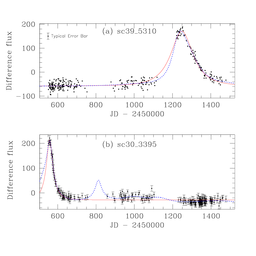
Figure 1: Two events which highlight the problems associated with noisy data. The solid and dotted lines represent the standard fit and the parallax fit, respectively. (a) The event sc39_5310, which illustrates how slight deviations between the two fits can easily be hidden by noisy data. The error bars have been omitted for clarity, but a typical error bar is shown in the top left hand corner. (b) The event sc30_3395, which demonstrates how a microlensing light-curve can be seemingly-erroneously fitted with a parallax model exhibiting many peaks. This leads to a significant improvement in $\chi^{2}$. Such multi-peak parallax models often occur in events with noisy data, which may signal additional variability other than microlensing.

However, more than two thirds of these events still turn out to have noisy data and are unsuitable for detecting parallax signatures. A typical example of this is given in Fig. 1(a), which clearly illustrates the fact that more accurate data are needed in order to observe the often slight deviations between the standard and parallax fits. Another common problem which occurs with the noisy events is shown in Fig. 1(b). In this case, the parallax fit substantially improves the $\chi^{2}$ because the parallax fit has multiple peaks that better reproduce the fluctuations in the data. However, one notices that the secondary peak falls in a gap between two observing seasons. Many other parallax fits for the noisy events show similar multiple-peak structures. While such multi-peak parallax events have been predicted (Gould et al. 1994), the large error bars make the identification un-convincing. This is further supported by their often unusual parameter values; for example, the majority of these events have values of $\tilde{r}_{\rm E}$ which are significantly different from the value of a few AU which is expected for a typical microlensing event. It is therefore clear that the identification of parallax signatures requires accurate data in order to observe the slight deviations and so the light curves for these noisy events were of little use and we do not regard them as parallax events. To eliminate these events from our selection procedure we needed to quantify how noisy the data were for an event. This was done by analysing the signal-to-noise ratio. To assess this signal-to-noise ratio, we use a quantity, $({\rm S/N})_{\rm peak}$, defined as the difference between the peak flux and the baseline flux divided by the average error estimated using the data points outside the ‘duration’ of the light curve. We find empirically that $({\rm S/N})_{\rm peak}>30$ provides an excellent separator. This criterion, while satisfactory, is somewhat arbitrary; we return to this issue briefly in the discussion.

As well as identifying events which displayed parallax signatures, we also wished to find events which unexpectedly exhibited no deviations from the standard light curve. Of particular interest are events which have unusually large time-scales but no signs of asymmetry, since they provide lower-limits on $\tilde{r}_{\rm E}$ (see §4.3). To isolate these we used the event duration which was mentioned earlier. We also used two further criteria: firstly, a measure of the improvement in $\chi^{2}$ between the standard and the parallax fits (i.e. a high value of $p_{F}$, which corresponds to no significant improvement in $\chi^{2}$) and secondly, the signal-to-noise ratio, $({\rm S/N})_{\rm peak}$. Events which had duration $>100$ days, $({\rm S/N})_{\rm peak}>30$, and probability $p_{F}>0.05$ were considered as long-duration events that showed no parallax signatures.

4 Results

Out of the 512 events, there were 8 events where the incorporation of the parallax effect substantially improved the goodness of the fit (see above) and passed our test of event duration and the peak signal-to-noise ratio. These events are given in Table 1. One light curve was found to show clear signs of parallax affected behaviour, in addition to a number of others which could be classified as marginal cases. In the following, we shall first discuss these parallax candidates and in §4.3 we discuss the physical limits that one can derive from the long-duration events that exhibited no parallax signatures.

For all the microlensing events presented here, we re-normalize the $\chi^{2}$ per degree of freedom to be unity for the best-fitting model by multiplying the quoted observational errors by a constant factor (usually between 0.8 to 1.3). This is necessary because we found that the quoted error bars in observations are often too large. The events in §4.1 and §4.2 were re-normalized using the best-fitting parallax model, while the events in §4.3 were re-normalized using the best-fitting standard model (which has essentially the same $\chi^{2}$ as the best-fitting parallax model). This re-normalization affects primarily the quoted error bars in the model parameters. It also weakly affects the selection procedure through both the peak flux ratio, $({\rm S/N})_{\rm peak}$, and duration, although this perturbation is only very slight since $l$ in eq. (5) remains unchanged.

4.1 Parallax microlensing candidate

From the catalogue of 512 microlensing events, the most convincing parallax event we found was sc33_4505, which is shown in Fig. 2. Despite the lack of data for two important regions (namely $t\equiv{\rm JD}-2450000<550$ days and $760<t<870$ days), the systematic deviations from the standard curve can clearly be seen. During the upward slope of the light curve the standard fit undoubtedly has a gradient which is too shallow and yet for the downward slope this fit’s gradient is clearly too steep. This prominent asymmetry provides strong evidence that the light curve may be exhibiting parallax behaviour and this is further supported when the parallax model is used to fit the data. This model provides a much more accurate fit, with the $\chi^{2}$ being drastically reduced from 398.972 (or $\chi^{2}=2.23$ per degree of freedom) to 177 ($\chi^{2}=1$ per degree of freedom). When observing resumed after $t=870$ days it can be seen that the parallax model fitted this region more accurately, even though the lensing event was very nearly over and the magnification was only a fraction of the peak value.

The best fit parameters from both the standard and parallax fit are given in Table 2. In particular, for the best-fitting parallax model, we find that

$$t_{\rm E}=194\pm 30\,{\rm days},~{}~{}\tilde{r}_{\rm E}=6.37\pm 0.53\,{\rm AU}.$$ (6)

An expression for the lens mass as a function of the relative lens-source distance can be shown to be (see Soszyński et al. 2001),

$$M=\frac{c^{2}\tilde{r}_{\rm E}^{2}}{4G}\left({{1\over D_{\rm l}}-{1\over D_{\rm s}}}\right)=0.0123M_{\odot}\left(\frac{\tilde{r}_{\rm E}}{\rm AU}\right)^{2}\left(\frac{\pi_{\rm rel}}{0.1\rm mas}\right),~{}~{}\pi_{\rm rel}\equiv{{{\rm AU}\over D_{\rm l}}-{{\rm AU}\over D_{\rm s}}},$$ (7)

where $\pi_{\rm rel}$ is the relative lens-source parallax in milli-arcseconds. For this event, the parallax parameters give a projected velocity of

$$\tilde{v}=\frac{\tilde{r}_{\rm E}}{t_{\rm E}}=57^{+16}_{-12}\mbox{ km s}^{-1}.$$ (8)

The lens mass depends on the relative lens-source parallax (eq. 7). If the source is about 7 kpc away, and the lens lies in the disk half-way between the observer and the source ($x=1/2$), then $\pi_{\rm rel}\approx 0.143$ mas, which gives a lens mass of about $0.71M_{\odot}$; as a comparison, for a bulge self-lensing event with $D_{\rm s}\approx 8\,\rm{kpc}$ and $D_{\rm l}\approx 6\,\rm{kpc}$, then $\pi_{\rm rel}\approx 0.042$ mas, which would give a lens mass of about $0.21M_{\odot}$. However, this latter scenario is less likely since the projected velocity of the lens is relatively low. It appears that similar to the previous parallax microlensing events, this event is caused by a slow-moving and likely low-mass lens.

4.2 Marginal parallax microlensing candidates

Apart from the above convincing candidate, sc33_4505, a number of events were found which showed indications of parallax signatures. However, the case for classifying these events as having parallax affected light curves is not wholly convincing, mainly due to the insufficiency of the data. Figs. 3-9 show these ‘marginal’ microlensing events that we have found, and Table 3 presents the best fit parameters for both the standard and parallax models.

The problem of insufficient sampling is clear from several marginal cases. For example, for the sc41_3299 event (Fig. 8), there are very few points in the rising branch of the light curve. As a result, although the parallax fit seems to provide a somewhat better fit in the region between $t=880-900$ days, it is not clear whether this is a genuine parallax event or just due to the large errors in the data. The situation is similar for events sc20_5748 (Fig. 4), sc27_3078 (Fig. 6), and sc43_836 (Fig. 9). For the event sc6_2563 (Fig. 3), the standard fit consistently over-predicts the fluxes between $t=1040$ to $1140$ days, and the parallax model provides a much better fit for these parts. Unfortunately, there was no data for the time period ($t\sim$ 1180 days) when the standard model and the parallax model are predicted to show substantial deviations. The fact that we can pick out marginal cases like sc41_3299 implies that our selection method is sensitive, and it is unlikely that we could have missed many true candidate parallax events.

The situations for the events sc20_5875 (Fig. 5) and sc35_2526 (Fig. 7) are slightly different. For the sc35_2526 event, the light curve is highly asymmetric, and the standard model is clearly a bad fit. The parallax model, on the other hand, provides a much better fit; the improvement in $\chi^{2}$ is from 361.5 to 170. However, the fit is not perfect, particularly at the peak and for the few data points between $700<t<750$ days. For this reason, we still cautiously regard this event as a “marginal” parallax candidate event. The situation for sc20_5875 is similar, but less dramatic. It is possible that these two events are produced by binaries, where the asymmetry is provided, e.g., by the shear perturbation by the secondary on the primary lens (e.g. Mao & Di Stefano 1995). Notice that, for the event sc35_2526, the $t_{\rm E}$ parameter is unusually long (see Table 3); however, this is just an artifact due to the well-known degeneracy between the impact parameter, $u_{0}$, and $t_{\rm E}$ for microlensing light curves in blended light curves (Woźniak & Paczyński 1997), where only the combination of $u_{0}t_{\rm E}$ can be inferred in some cases.

4.3 Long microlensing events that show no parallax signatures

Of almost equal interest to parallax events are the events which have large time-scales and yet exhibit no signs of parallax induced asymmetry. A total of 20 events were identified using the selection criteria which were given in §3, i.e. events which had duration $>100$ days, $({\rm S/N})_{\rm peak}>30$, and probability $p_{F}>0.05$. The parallax signatures become more pronounced for small values of $\tilde{r}_{\rm E}$ because the Earth’s motion around the Sun then becomes a larger fraction of the Einstein radius, and hence presents a larger perturbation to the light curve. The lack of parallax signatures therefore provides a lower-limit on $\tilde{r}_{\rm E}$. For each such event, we fix $\tilde{r}_{\rm E}$ in a range of values while letting all the other six parameters vary and find the minimum $\chi^{2}$ value for each fixed $\tilde{r}_{\rm E}$. The $2\sigma$ confidence constraint on $\tilde{r}_{\rm E}$ is then given by the $\tilde{r}_{\rm E}$ value corresponding to the point at which its $\chi^{2}$ becomes larger than the best fit $\chi^{2}$ by 4.00 (e.g. Lupton 1993). From eq. (7), one sees that this lower limit on $\tilde{r}_{\rm E}$ can then be translated into a lower limit on $M/\pi_{\rm rel}$. The events which produced the 4 largest constraints are given in Table 4, and their light curves are shown in Fig. 10.

In all cases, the lower limits on the mass are rather weak, the best case being for event sc26_2218, where the lower limit reaches about $0.2M_{\odot}$ for $\pi_{\rm rel}=0.1$ mas. These weak constraints are similar to those found by the EROS collaboration for the microlensing event EROS2-GSA1 (Derue et al. 1999), from which they obtained values of $\tilde{r}_{\rm E}\geq 1.33$ AU and $M\ga 10^{-3}M_{\odot}$.

5 Summary and discussion

We have conducted an extensive search for parallax events in the microlensing database of 512 microlensing events obtained by the difference image analysis of the OGLE II data. Our selection procedure involves a direct comparison of the standard microlensing model and the parallax model, augmented by the requirements of long duration and high peak signal-to-noise ratio. While empirically we found these criteria to be very effective, there is no guarantee that these selection procedures are optimal. This issue is best explored using the recovery of artificial parallax events in Monte Carlo simulations (see below).

Using our selection criteria, we found one convincing new parallax microlensing event, sc33_4505. A number of other more marginal cases were also recovered. However, while these marginal events are better fitted by a model incorporating the parallax effect, their parallax nature cannot be established beyond any doubt due to the poor sampling in the light curve. This may be particularly severe for the events which last for about one year, due to the gap of approximately three months between observing seasons. In such cases either the rising or the declining branch of the light curve will typically be missing, and so the parallax induced asymmetry is particularly difficult to identify. We have also found some very long events that showed no parallax signatures, and these events provide a lower-limit on the Einstein radius projected onto the observer plane. Consequently, a lower-limit on the lens mass $M/\pi_{\rm rel}$ can be derived (cf. eq. 7). However, in most cases, the lower limits on $M/\pi_{\rm rel}$ are rather weak.

The convincing parallax event (sc33_4505) is similar to all of the other 4 known parallax events (see introduction) in that it is caused by a slow-moving lens and, quite likely, a low mass lens. The low projected velocity favors the interpretation that this microlensing geometry is a disk source lensed by a disk lens. For such events, the observer, the lens and the source rotate about the Galactic center with roughly the same velocity, and the relative motion is only due to the small, $\sim 10{\rm\,km\,s^{-1}}$, random velocities (see, e.g. Derue et al. 1999). On the other hand, the chance for a bulge source (with its much larger random velocity, $\sim 100{\rm\,km\,s^{-1}}$) to have such a low projected velocity relative to the lens (whether in the disk or bulge) is small. So it appears that all known parallax events are caused by disk-disk lensing. If this is true, then the radial velocities of the lensed sources are expected to be small. It will therefore be very interesting to check this by obtaining the radial velocities of the parallax events spectroscopically. Since their projected transverse velocities are known, one obtains a more complete kinematic picture of these unusual microlensing events that can be used to probe the dynamical model of the Milky Way. As a by product, one also obtains the metallicity and age of these stars.

While the number of convincing parallax events toward the Galactic bulge seems to be very low (1 out of 512), the number of marginal cases makes the true fraction somewhat uncertain. A related question is whether existing microlensing catalogs are biased against parallax events. This is an important issue because parallax events preferentially have long durations, which may be detectable only when one has monitored the stars for many years. In fact, after the completion of this work, eight additional events were recovered by cross identification of the 214 microlensing candidates from the standard OGLE database with the difference image analysis variability database of Woźniak (2000). Some of these were missed in the first search because they have such long durations that they have not yet reached a constant baseline. We plan to analyze these additional unique events for parallax signatures. On the theoretical side, Buchalter & Kamionkowski (1997) have estimated the expected fraction of parallax events which would be identified, using a regular sampling of every few minutes to $\sim 1$ day. Our search strongly suggests that the irregular sampling and gaps between different observing seasons hamper the recovery of parallax events. We plan to perform a simulation with realistic sampling and photometric errors similar to those found in observations. A comparison between the observed and predicted rates may enable us to provide constraints on the lens and source kinematics. Such simulations will also be helpful for devising the optimal search strategy for selecting parallax events from the experiments. The results of these Monte Carlo simulations will be reported in a future publication.

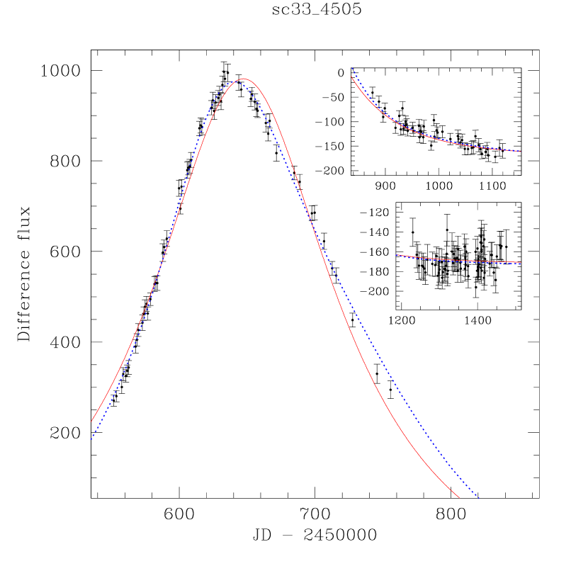
Figure 2: Difference flux ($f(t)$, as defined in eq. 4) as a function of time for the best candidate parallax microlensing event, sc33_4505. The solid line shows the best standard fit while the dotted line shows the best fit that accounts for the parallax effect. The insets show the light curves for the ‘non-lensed’ seasons.

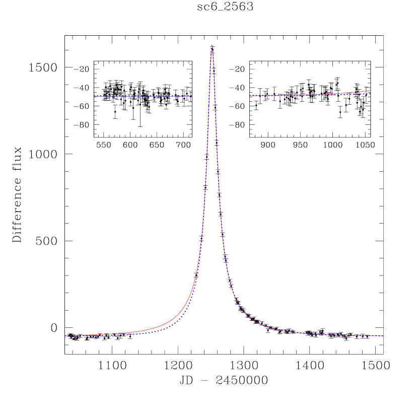
Figure 3: The marginal candidate parallax microlensing event, sc6_2563. The notations are the same as in Fig. 2.

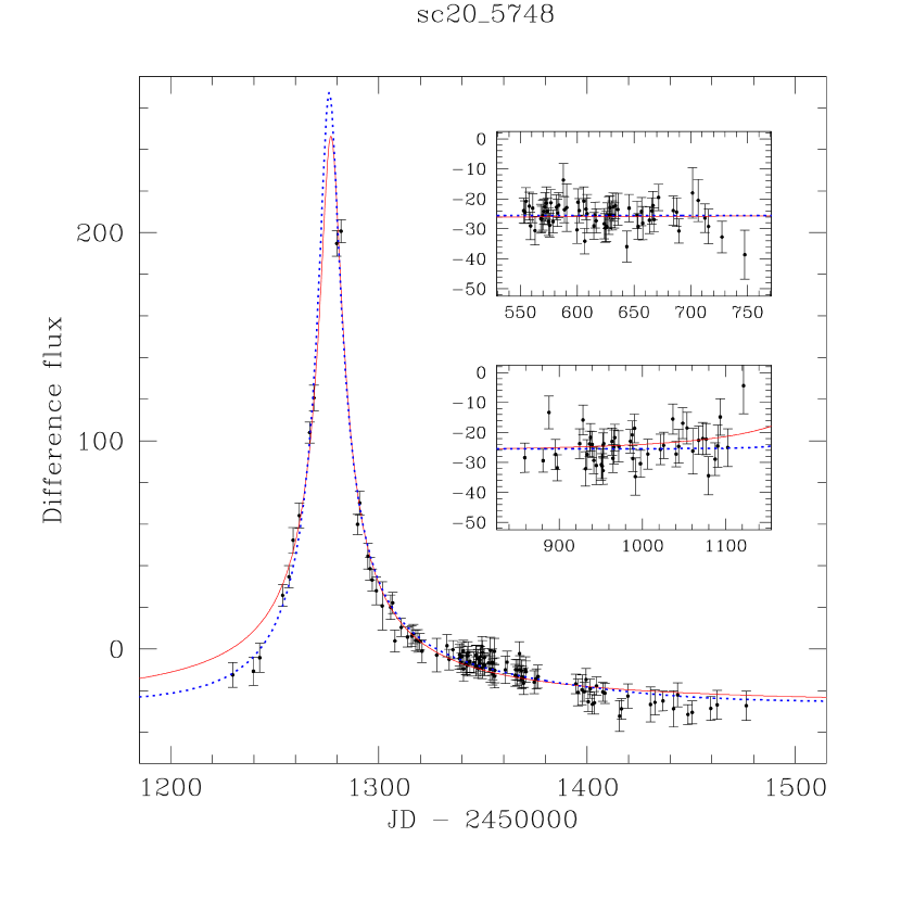
Figure 4: The marginal candidate parallax microlensing event, sc20_5748. The notations are the same as in Fig. 2.

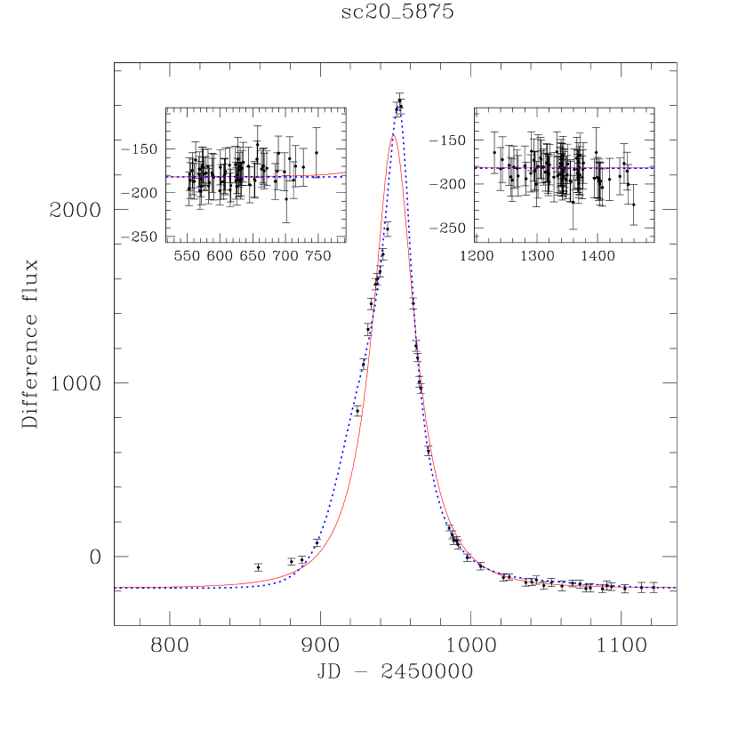
Figure 5: The marginal candidate parallax microlensing event, sc20_5875. The notations are the same as in Fig. 2. This event is not perfectly fit by the parallax model. This event may, instead, be caused by a (weak) binary lens (see also Fig. 7).

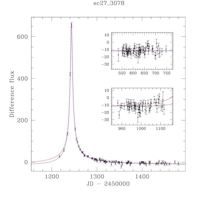
Figure 6: The marginal candidate parallax microlensing event, sc27_3078. The notations are the same as in Fig. 2.

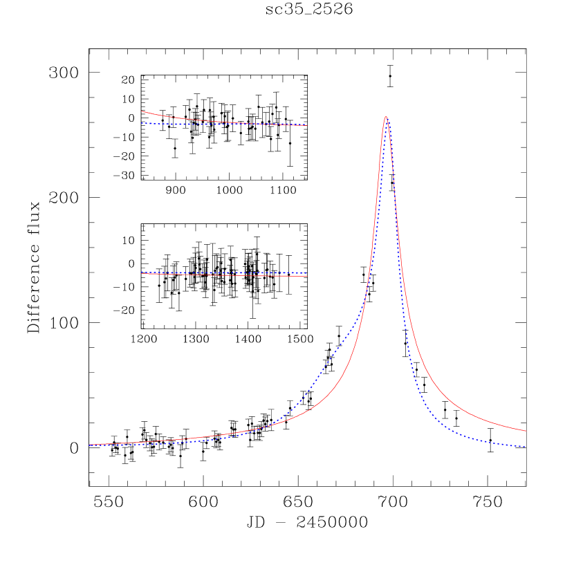
Figure 7: The marginal candidate parallax microlensing event, sc35_2526. The notations are the same as in Fig. 2. This event is not perfectly fit by the parallax model. This event may, instead, be caused by a (weak) binary lens (see also Fig. 5).

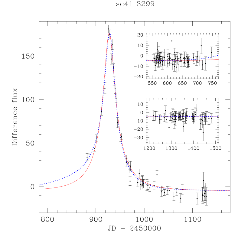
Figure 8: The marginal candidate parallax microlensing event, sc41_3299. The notations are the same as in Fig. 2.

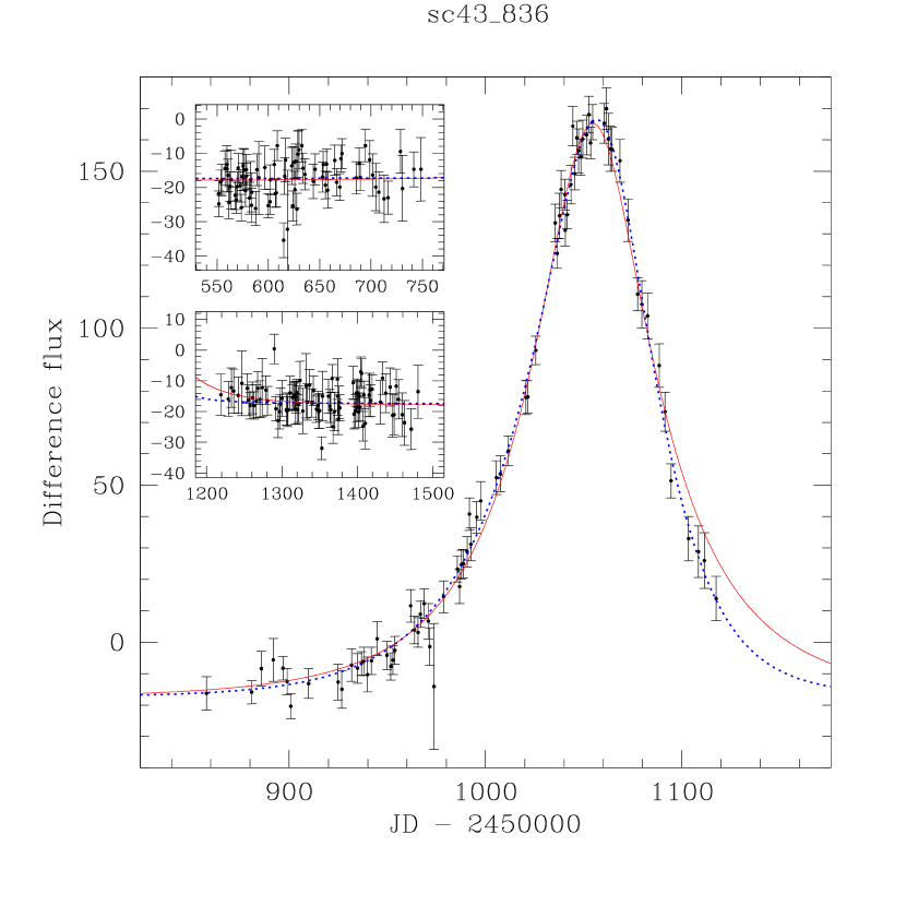
Figure 9: The marginal candidate parallax microlensing event, sc43_836. The notations are the same as in Fig. 2.

Figure 10: The 4 long-duration lensing events which produced the most stringent lower-limits on the lens mass $M/\pi_{\rm rel}$ (see eq. 7 and Table 4). For these events, the incorporation of parallax effects produces virtually no improvement in the $\chi^{2}$. The dotted line shows the theoretical baseline flux and the horizontal axis covers a length of time corresponding to the event duration, as specified in §3.

Table 1: The 8 events which were systematically selected as potential parallax affected light-curves, and their subsequent classification. The probability $p_{F}$ and $({\rm S/N})_{\rm peak}$ are defined in §3. The convincing candidate (sc33_4505) and other marginal candidates are shown in Figs. 2-9.

Event	RA	DEC	Duration (day)	$t_{\rm E}$ (day)	$p_{F}$	$({\rm S/N})_{\rm peak}$	Classification
sc6_2563	18:08:02.64	-31:49:05.2	$245$	$66.6\pm 1.3$	$1.22\times 10^{-8}$	228.39	marginal
sc20_5748	17:59:39.05	-28:27:16.6	$150$	$78.2\pm 2.5$	$2.58\times 10^{-5}$	38.99	marginal
sc20_5875	17:59:08.99	-28:24:54.7	$146$	$27.22\pm 0.21$	$0.00$	119.04	marginal/binary?
sc27_3078	17:48:15.92	-34:50:09.0	$162$	$124\pm 10$	$2.04\times 10^{-7}$	142.82	marginal
sc33_4505	18:05:46.71	-28:25:32.1	$663$	$194\pm 30$	$5.78\times 10^{-32}$	78.79	convincing
sc35_2526	18:04:22.42	-27:57:52.2	$162$	$6600\pm 180$	$1.44\times 10^{-28}$	47.02	marginal/binary?
sc41_3299	17:52:19.08	-32:48:20.8	$119$	$98\pm 18$	$1.28\times 10^{-5}$	35.17	marginal
sc43_836	17:34:52.64	-27:23:14.4	$207$	$45.1\pm 1.6$	$4.31\times 10^{-5}$	31.70	marginal

Table 2: The best standard model (first row) and the best parallax model (second row) for the convincing candidate sc33_4505.

Model	$t_{0}$	$t_{\rm E}$ (day)	$u_{0}$	$f_{\rm L}$	$\Delta f$	$\psi$	$\tilde{r}_{\rm E}$ (AU)	$\chi^{2}$
S	$647.22\pm 0.36$	$166\pm 11$	$-0.412\pm 0.036$	$730\pm 91$	$-172.2\pm 1.8$	—	—	399.0
P	$654.4\pm 4.1$	$194\pm 30$	$-0.207\pm 0.065$	$440\pm 150$	$-174.3\pm 2.1$	$3.136\pm 0.011$	$6.37\pm 0.53$	177

Table 3: The best standard model (indicated by ‘S’) and the best parallax model (indicated by ‘P’) for marginal parallax candidates. The error bars have been rescaled so as to enforce the $\chi^{2}$ per degree of freedom to be unity for the best-fitting parallax model.

Event	$t_{0}$	$t_{\rm E}$ (day)	$u_{0}$	$f_{\rm L}$	$\Delta f$	$\psi$	$\tilde{r}_{\rm E}$ (AU)	$\chi^{2}$
sc6_2563,S	$1251.971\pm 0.068$	$89.2\pm 2.8$	$0.0758\pm 0.0032$	$135.9\pm 5.7$	$-49.43\pm 0.52$	—	—	253.7
————,P	$1263.85\pm 0.62$	$66.6\pm 1.3$	$0.0272\pm 0.0085$	$192.8\pm 5.5$	$-48.84\pm 0.49$	$0.262\pm 0.012$	$4.27\pm 0.16$	214
sc20_5748,S	$1277.03\pm 0.22$	$357\pm 120$	$-0.0148\pm 0.0056$	$4.1\pm 1.5$	$-26.24\pm 0.67$	—	—	243.2
————,P	$1315.12\pm 0.96$	$78.2\pm 2.5$	$-0.325\pm 0.041$	$16.67\pm 0.79$	$-25.50\pm 0.41$	$1.234\pm 0.057$	$2.43\pm 0.11$	221
sc20_5875,S	$948.74\pm 0.10$	$31.3\pm 1.7$	$0.461\pm 0.042$	$1950\pm 250$	$-181.9\pm 1.7$	—	—	666.7
————,P	$933.88\pm 0.28$	$27.22\pm 0.21$	$2.073\pm 0.011$	$320\pm 25$	$-182.0\pm 1.6$	$0.235\pm 0.011$	$0.3515\pm 0.0021$	189
sc27_3078,S	$1243.481\pm 0.077$	$312\pm 77$	$0.0070\pm 0.0018$	$4.8\pm 1.2$	$-12.08\pm 0.52$	—	—	245.2
————,P	$1238.75\pm 0.34$	$124\pm 10$	$-0.6266\pm 0.0068$	$18.2\pm 1.3$	$-11.60\pm 0.36$	$2.971\pm 0.026$	$1.68\pm 0.019$	212
sc35_2526,S	$696.33\pm 0.20$	$53000\pm 11000$	$0.000107\pm 0.000021$	$0.0291\pm 0.0057$	$-7.39\pm 0.59$	—	—	361.5
————,P	$695.46\pm 0.23$	$6600\pm 180$	$0.01512\pm 0.00018$	$0.0920\pm 0.0066$	$-4.65\pm 0.57$	$2.9967\pm 0.0087$	$63.02\pm 0.73$	170
sc41_3299,S	$927.65\pm 0.29$	$63.2\pm 8.3$	$0.186\pm 0.034$	$40.8\pm 8.5$	$-4.63\pm 0.40$	—	—	197.1
————,P	$913.1\pm 7.7$	$98\pm 18$	$0.19\pm 0.16$	$26.2\pm 6.8$	$-4.87\pm 0.47$	$6.222\pm 0.096$	$2.33\pm 0.68$	173
sc43_836,S	$1054.69\pm 0.41$	$71.5\pm 7.2$	$0.437\pm 0.067$	$126\pm 28$	$-17.91\pm 0.41$	—	—	262.0
————,P	$1040.0\pm 1.6$	$45.1\pm 1.6$	$-0.104\pm 0.035$	$176\pm 13$	$-17.38\pm 0.37$	$3.1744\pm 0.0054$	$1.511\pm 0.091$	241

Table 4: The 4 non-lensed events which produced the best $2\sigma$ confidence lower limit on the projected Einstein radius in the observer plane ($\tilde{r}_{\rm E}$) and on $M/\pi_{\rm rel}$ (cf. eq. 7). The ‘duration’ of the event is defined in §3, and the probability $p_{F}$ is defined below eq. (5). The relative lens-source parallax $\pi_{\rm rel}$ is in units of milli-arcseconds; for microlensing events toward the Galactic bulge, $\pi_{\rm rel}\sim 0.1$ mas.

Event	RA	DEC	Duration (day)	$t_{\rm E}$ (day)	$p_{F}$	$\tilde{r}_{\rm E}$ (AU)	$M/\pi_{\rm rel}$ ($M_{\odot}$)
sc22_1992	17:56:35.30	-30:56:33.4	$151$	$45.5\pm 3.7$	$0.132$	$0.94$	$0.11$
sc26_2218	17:47:23.29	-34:59:52.4	$195$	$45.10\pm 0.59$	$0.104$	$3.74$	$1.71$
sc34_3906	17:58:37.11	-29:06:29.9	$331$	$58.7\pm 6.2$	$0.204$	$1.44$	$0.25$
sc45_810	18:03:30.06	-30:09:55.6	$115$	$98\pm 54$	$0.151$	$1.73$	$0.37$

References

- [1]
- [2] Alard C., Lupton R. H., 1998, ApJ, 503, 325
- [3] Alard C., 2000, A&A Suppl., 144, 363
- [4] Alcock C. et al., 1995, ApJ, 454, L125
- [5] Alcock C. et al., 2000a, ApJ, 541, 270
- [6] Alcock C. et al., 2000b, ApJ, 542, 281
- [7] Bennett D. P. et al., 1997, BAAS, 191, 8303
- [8] Bond I. A. et al. (the MOA collaboration) 2001, preprint (astro-ph/0102181)
- [9] Buchalter A., Kamionkowski M., 1997, ApJ, 482, 782
- [10] Derue F. et al., 1999, A&A, 351, 87
- [11] Dominik M., 1998, A&A, 329, 361
- [12] Gould A., 1992, ApJ, 392, 442
- [13] Gould A., 1994, ApJ, 421, L71
- [14] Gould A., Miralda-Escude J., Bahcall J.N., 1994, ApJ, 423, L105
- [15] Lupton R. H., 1993, Statistics in theory and practice (Princeton: Princeton University Press)
- [16] Mao S., Paczynski B., 1991, ApJ, 374, L37.
- [17] Mao S., Di Stefano R., 1995, ApJ, 440, 22
- [18] Mao S., 1999, A&A, 350, L19
- [19] Nemiroff R.J., Wickramasinghe W.A.D.T., 1994, ApJ, 424, L21
- [20] Paczyński B., 1986, ApJ, 304, 1
- [21] Paczyński B., 1996, ARAA, 34, 419
- [22] Refsdal S., 1966, MNRAS, 134, 315
- [23] Sahu K. C., 1994, Nature, 370, 275
- [24] Soszyński I. et al., 2001, ApJ, 552, 731
- [25] Udalski A., Kubiak M., Szymański M., 1997, Acta Astron., 47, 319
- [26] Udalski A., Żebruń K., Szymański M., Kubiak M., Pietrzyński G., Soszyński I., Woźniak P., 2000, Acta Astron., 50, 1
- [27] Witt H.J., Mao S., 1994, ApJ, 430, 505
- [28] Woźniak P., Paczyński B., 1997, ApJ, 487, 55
- [29] Woźniak P., 2000, Acta Astron., 50, 421
- [30] Woźniak P. et al., 2001, Acta Astron., submitted (astro-ph/0106474)
- [31] Zhao H.S., Evans W.N., 2000, ApJ, 545, L35