Self-consistent axisymmetric Sridhar–Touma models

Abstract

We construct phase-space distribution functions for the oblate, cuspy mass models of Sridhar & Touma, which may contain a central point mass (black hole) and have potentials of Stäckel form in parabolic coordinates. The density in the ST models is proportional to a power $r^{-\gamma}$ of the radius, with $0<\gamma<1$. We derive distribution functions $f(E,L_{z})$ for the scale-free ST models (no black hole) using a power series of the energy $E$ and the component $L_{z}$ of the angular momentum parallel to the symmetry axis. We use the contour integral method of Hunter & Qian to construct $f(E,L_{z})$ for ST models with central black holes, and employ the scheme introduced by Dejonghe & de Zeeuw to derive more general distribution functions which depend on $E$, $L_{z}$ and the exact third integral $I_{3}$. We find that self-consistent two- and three-integral distribution functions exist for all values $0<\gamma<1$.

1 Introduction

Observations of the nuclei of elliptical galaxies using the Hubble Space Telescope have revealed that the luminosity density diverges towards the centre as a power $r^{-\gamma}$ of the radius [Jaffe et al. 1994, Lauer et al. 1995, Carollo et al. 1997, Rest et al. 2001]. Many and perhaps all of the nuclei host a central black hole [Richstone et al. 1999, de Zeeuw 2001]. Dynamical models for such cusped galaxies include the axisymmetric power-law galaxies introduced by Toomre (1982) and Evans (1994), which have spheroidal potentials and simple $f(E,L_{z})$ distribution functions, with $E$ the orbital energy and $L_{z}$ the component of the angular momentum parallel to the symmetry axis. Similar models with spheroidal densities were constructed by Dehnen & Gerhard (1994) and Qian et al. (1995, hereafter Q95). Most orbits in these models admit an approximate third integral of motion. Self-consistent three-integral distribution functions were constructed for some special scale-free cases by Schwarzschild’s (1979) numerical orbit superposition method (Richstone 1980, 1984; Levison & Richstone 1985) and by analytic means (de Zeeuw, Evans & Schwarzschild 1996; Evans, Häfner & de Zeeuw 1997, hereafter EHZ).

Q95 constructed two-integral distribution functions $f(E,L_{z})$ for axisymmetric power-law spheroidal densities containing a central black hole by means of the contour integral method of Hunter & Qian (1993, hereafter HQ). They showed that self-consistent $f(E,L_{z})$’s exist for oblate scale-free spheroids with $0\leq\gamma<3$, but found an upper bound for the axial ratios of self-consistent prolate models of this kind. Their study also revealed that the presence of a central black hole limits the region of parameter space for which physical distribution functions (i.e., $f(E,L_{z})\geq 0$) exist to $\gamma\geq 1/2$ (for all axis ratios). De Bruijne et al. (1996) studied oblate spheroidal cusps in the radial range where the spherical potential of the black hole dominates, and constructed analytic constant-anisotropy three-integral distribution functions $f(E,L_{z},L)$, with $L$ the modulus of the angular momentum. These distribution functions remain physical also when $0\leq\gamma<1/2$, and suggest that shallow-cusped axisymmetric galaxies with central black holes can in fact be constructed, a result confirmed by application of Schwarzschild’s numerical method (Verolme, priv. comm.). Self-consistent axisymmetric models with central black holes designed to fit the observed photometry and kinematics of specific galaxies were constructed with Schwarzschild’s method by, e.g., van der Marel et al. (1998), Cretton et al. (1999, 2000) and Gebhardt et al. (2000).

The oblate models introduced by Sridhar & Touma (1997a, hereafter ST) provide the only set of cuspy models with a central black hole for which all orbits have an exact third integral of motion $I_{3}$, so that, in principle, exact distribution functions can be constructed. The potential of these models is of Stäckel form in parabolic coordinates, and this causes the density to be significantly flattened, with a shape that is fixed once the cusp slope is chosen, and a total mass that is infinite. The oblate axisymmetric models with a potential of Stäckel form in prolate spheroidal coordinates [Kuzmin 1956, de Zeeuw 1985] also admit an exact third integral and include a large set of models with a range of density profiles and shapes with finite total mass. However, they all have constant density cores and can not contain a central point mass without destroying the separability [de Zeeuw, Peletier & Franx 1986]. Oblate density distributions with potentials that are separable in spherical coordinates have densities that become negative at large distances (Lynden–Bell 1962b). Here we study self-consistent distribution functions for the oblate ST models. We show that, by contrast to the cusped spheroidal densities of Q95, the ST models with a central black hole do have consistent $f(E,L_{z})$ distribution functions for all values of the cusp slope $0<\gamma<1$.

In §2 we summarize the properties of the ST models. Without a black hole, the ST models are scale-free. We discuss their distribution functions in §3, and investigate the general case in §4. We summarize our conclusions in §5.

2 Sridhar–Touma models

A comprehensive description of the mass models and the orbit structure can be found in ST. Here we collect the relevant properties, derive the fundamental integral equation for the distribution function, and close with a brief discussion of the velocity moments.

2.1 Potential, density and orbits

The motion in the axisymmetric ST models separates in parabolic coordinates $(\xi,\eta)$ in the meridional plane. We define them as

$$\xi=r(1+\cos\theta),\quad\eta=r(1-\cos\theta),\quad\xi,\eta\geq 0,$$ (1)

where $r$ is the polar radius and $\theta$ is the co-latitude. Our definition of $\eta$ differs from that in ST by an overall sign, which removes the need to use $|\eta|$ in many expressions. In these coordinates the gravitational potential of an ST model can be written as

$$V(\xi,\eta)=\frac{2K(\xi^{3-\gamma}+\eta^{3-\gamma})-2GM}{\xi+\eta},\quad K>0,$$ (2)

where $K$ is a positive constant, $G$ is the gravitational constant, and $M$ denotes the mass of a central black hole (point mass). The density distribution $\rho(\xi,\eta)$ associated with the potential (2) follows from eq. (18) of ST. When $M=0$, the potential and the density are proportional to $r^{2-\gamma}$ and $r^{-\gamma}$, respectively, i.e., they are scale-free, but the density is non-negative only for $0<\gamma<1$. The equipotential surfaces are approximately spheroidal. Their axis ratio $b/a$ (defined by the condition $V(0,b)=V(a,0)$) equals 1/2 for all values of $\gamma$. As a result, the surfaces of constant density are dimpled along the short ($z$) axis, and the dimple deepens, i.e., the density distribution becomes increasingly toroidal, with increasing $\gamma$.

For subsequent use, we record here the expressions for the ST potential-density pairs in terms of the standard spherical polar coordinates $(r,\theta,\phi)$

$$V(r,\theta)\!\!\! = \!\!\!Kr^{2-\gamma}P(\theta)-\frac{GM}{r},$$

$$\rho(r,\theta)\!\!\! = \!\!\!\rho_{0}r^{-\gamma}S(\theta)+M\delta(r),$$ (3)

where $\rho_{0}=2(3-\gamma)(1-\gamma)K/\pi G$, $\delta$ is the Dirac delta-function, and

$$P(\theta)\!\!\! = \!\!\!(1\!+\!\cos\theta)^{3-\gamma}+(1\!-\!\cos\theta)^{3-\gamma},$$

$$S(\theta)\!\!\! = \!\!\!(2\!-\!\gamma\!-\!\cos\theta)(1\!+\!\cos\theta)^{2-\gamma}$$ (4)

$$\!\!\!+(2\!-\!\gamma\!+\!\cos\theta)(1\!-\!\cos\theta)^{2-\gamma}.$$

In terms of cylindrical polar coordinates ($\varpi,\phi,z$):

$$V(\varpi,z)\!\!\!\! = \!\!\!\!\frac{K}{r}\big{[}(r\!+\!z)^{3-\gamma}\!+\!(r\!-\!z)^{3-\gamma}\big{]}-\frac{GM}{r},$$

$$\rho(\varpi,z)\!\!\!\! = \!\!\!\!\frac{\rho_{0}}{r^{3}}\big{\{}[(2-\gamma)r\!\!-\!\!z](r\!+\!z)^{2-\gamma}$$ (5)

$$\!+[(2-\gamma)r\!+\!z](r\!\!-\!\!z)^{2-\gamma}\big{\}}\!+\!M\delta(r),$$

where $r=\sqrt{\varpi^{2}+z^{2}}$. In what follows, we take units such that $K=1$ and $\rho_{0}=1$.

The separation of the Hamilton-Jacobi equation results in a third integral of motion given by [Pars 1965]

$$I_{3}=2\xi p_{\xi}^{2}+2\xi^{3-\gamma}+\frac{L_{z}^{2}}{2\xi}-E\xi-GM,$$ (6)

or, equivalently

$$I_{3}=-2\eta p_{\eta}^{2}-2\eta^{3-\gamma}-\frac{L_{z}^{2}}{2\eta}+E\eta+GM,$$ (7)

with $p_{\xi}$ and $p_{\eta}$ the momenta conjugate to $\xi$ and $\eta$, respectively. Here $E$ denotes the orbital energy and $L_{z}\equiv p_{\phi}=r^{2}\dot{\phi}\,\sin^{2}\theta$ the component of the angular momentum parallel to the symmetry axis, both of which are integrals of motion as well. All orbits with $L_{z}\not=0$ are short-axis tubes, which may be either symmetric or asymmetric with respect to the equatorial plane. Those with $L_{z}=0$ are confined to a plane of constant $\phi$, and are centrophilic when a black hole is present. The orbital families are illustrated in Figure 2 of ST.

2.2 Distribution functions

In integrable systems, the distribution function depends on the phase-space coordinates through the isolating integrals of motion (Jeans 1915; Lynden–Bell 1962a), which for axisymmetric systems means $f=f(E,L_{z},I_{3})$. The mass density $\rho$ is related to $f$ through the integral

$$\!\!\!\!\!\!\!\rho(r,\theta)=\int\!\!f(E,\!L_{z},\!I_{3})\,{\rm d}^{3}\mn@boldsymbol{v}$$

$$\!\!\!=8\!\int\!\!\!{f(E,\!L_{z},\!I_{3})\over r^{2}\sin\theta}\left|\frac{\partial(\xi,\eta,\phi)}{\partial(r,\theta,\phi)}\!\frac{\partial(p_{\xi},p_{\eta},p_{\phi})}{\partial(E,I_{3},L_{z})}\right|{\rm d}E{\rm d}L_{z}{\rm d}I_{3},$$ (8)

where $\mn@boldsymbol{v}=(v_{r},v_{\theta},v_{\phi})^{\rm T}$ is the velocity vector in the spherical coordinates, and the factor of eight occurs because both $E$ and $I_{3}$ are quadratic in the velocities, and we consider only distribution functions that are even in $L_{z}$, so that $f(E,-L_{z},I_{3})=f(E,L_{z},I_{3})$. The Jacobians in the integral (2.2) follow from expressions (1), (6) and (7), and are given by

$$\frac{\partial(\xi,\eta,\phi)}{\partial(r,\theta,\phi)}\!\!\! = \!\!\!2r\sin\theta,$$

$$\left|\frac{\partial(p_{\xi},p_{\eta},p_{\phi})}{\partial(E,I_{3},L_{z})}\right|\!\!\! = \!\!\!\left|-\frac{\xi+\eta}{16\xi\eta p_{\xi}p_{\eta}}\right|$$ (9)

$$= \!\!\!\frac{1}{4\sin\theta\sqrt{[I_{3}\!-\!I_{3}^{-}][I_{3}^{+}\!-\!I_{3}]}},$$

where

$$I_{3}^{-}=I_{3}^{-}(E,L_{z},\xi)\!\!\! = \!\!\!2\xi^{3-\gamma}+\frac{L_{z}^{2}}{2\xi}-E\xi-GM,$$

$$I_{3}^{+}=I_{3}^{+}(E,L_{z},\eta)\!\!\! = \!\!\!-2\eta^{3-\gamma}-\frac{L_{z}^{2}}{2\eta}+E\eta+GM$$ (10)

We define the equivalent surface density $\Sigma(r,\theta)$ by

$$\Sigma(r,\theta)=2r\sin\theta\rho(r,\theta),$$ (11)

and substitute expression (2.2) in the integral (2.2) to obtain

$$\Sigma(r,\theta)=\!8\!\!\!\!\int\limits_{V(r,\theta)}^{\infty}\!\!\!\!\!{\rm d}E\!\!\!\!\!\!\int\limits_{0}^{{L_{z}}_{\rm max}(E,r,\theta)}\!\!\!\!\!\!\!\!\!\!\!{\rm d}L_{z}\int\limits_{I_{3}^{-}(E,L_{z},\xi)}^{I_{3}^{+}(E,L_{z},\eta)}\!\!\!\!\!\!\!\!\!\!{\rm d}I_{3}\!\frac{f(E,L_{z},I_{3})}{\sqrt{[I_{3}\!-\!I_{3}^{-}][I_{3}^{+}\!-\!I_{3}]}},$$ (12)

where

$${L_{z}}_{\rm max}(E,r,\theta)=r\sin\theta\sqrt{2[E-V(r,\theta)]}.$$ (13)

This is the fundamental integral equation for the distribution functions of the ST models. According to (13), the distribution functions obtained from (12) will be even in $L_{z}$. We assign only positive values to ${L_{z}}_{\rm max}$, which means that all stellar orbits have a definite sense of rotation around the axis of symmetry.

       

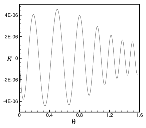
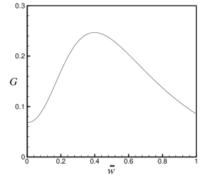
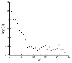
                          $(a)$ $(b)$ $(c)$

Figure 1: (a) The variation of $R(\theta)=\sigma(\theta)-\sigma_{N}(\theta)$ for $\gamma=0.7$ and $N=28$. (b) The distribution function ${\cal G}(\overline{w})$ for $0\leq\overline{w}=w/w_{\rm max}\leq 1$. (c) The history of the objective function ${\cal J}$ versus $N$. ${\cal J}$ has converged to its minimum at $\approx 10^{-12}$. The numerical accuracy is saturated because of truncation and round-off errors.

2.3 Velocity moments

The velocity moments $\rho\langle v_{\xi}^{l}v_{\eta}^{m}v_{\phi}^{n}\rangle$ are defined by

$$\rho\langle v_{\xi}^{l}v_{\eta}^{m}v_{\phi}^{n}\rangle\!=\!\!\int\!\!\int\!\!\int v_{\xi}^{l}v_{\eta}^{m}v_{\phi}^{n}f(\xi,\eta,v_{\xi},v_{\eta},v_{\phi})\,{\rm d}^{3}\mn@boldsymbol{v},$$ (14)

where the integrations are carried out over all possible velocities. The velocity components are related to the momenta in parabolic coordinates through

$$p_{\xi}\!=\!{\cal L}^{2}\dot{\xi}\!=\!{\cal L}v_{\xi},~{}~{}p_{\eta}\!=\!{\cal M}^{2}\dot{\eta}\!=\!{\cal M}v_{\eta},~{}~{}p_{\phi}\!=\!{\cal N}^{2}\dot{\phi}\!=\!{\cal N}v_{\phi},$$ (15)

where ${\cal L}$, ${\cal M}$ and ${\cal N}$ are the metric coefficients defined as

$${\cal L}^{2}={\xi+\eta\over 4\xi},~{}~{}{\cal M}^{2}={\xi+\eta\over 4\eta},~{}~{}{\cal N}^{2}=\xi\eta.$$ (16)

Transforming to the integration variables $E$, $L_{z}$ and $I_{3}$ gives (cf. eq. [12])

$$\!\!\!\!\!\rho\langle v_{\xi}^{l}v_{\eta}^{m}v_{\phi}^{n}\rangle=2^{2+\frac{l+m}{2}}\xi^{l-n-1\over 2}\eta^{m-n-1\over 2}(\xi+\eta)^{-(l+m)\over 2}$$

$$\!\!\!\!\times\int\!{f(E,L_{z},I_{3})L_{z}^{n}\over(I_{3}\!-\!I_{3}^{-})^{{1-l}\over 2}(I_{3}^{+}\!-\!I_{3})^{{1-m}\over 2}}\,{\rm d}I_{3}{\rm d}L_{z}{\rm d}E,$$ (17)

where the integration limits are identical to those of the integral (12).

We consider only the second moments. It is not difficult to show that the velocity ellipsoid is aligned with the parabolic coordinate system, so that $\langle v_{\xi}v_{\eta}\rangle=\langle v_{\xi}v_{\phi}\rangle=\langle v_{\eta}v_{\phi}\rangle=0$. This leaves three non-zero elements of the stress tensor, $\langle v_{\xi}^{2}\rangle$, $\langle v_{\eta}^{2}\rangle$, and $\langle v_{\phi}^{2}\rangle$, which are connected to the potential $V$ and the density $\rho$ by two Jeans equations,

$${\partial\rho\langle v_{\xi}^{2}\rangle\over\partial\xi}\!\!\!\!\! = \!\!\!\!\!{\rho\over 2\xi(\xi\!+\!\eta)}\big{[}\xi\langle v_{\eta}^{2}\rangle\!+\!(\xi+\eta)\langle v_{\phi}^{2}\rangle$$

$$-(2\xi+\eta)\langle v_{\xi}^{2}\rangle\big{]}\!-\!\rho{\partial V\over\partial\xi},$$

$${\partial\rho\langle v_{\eta}^{2}\rangle\over\partial\eta}\!\!\!\!\! = \!\!\!\!\!{\rho\over 2\eta(\xi\!+\!\eta)}\big{[}\eta\langle v_{\xi}^{2}\rangle\!+\!(\xi+\eta)\langle v_{\phi}^{2}\rangle$$ (18)

$$-(2\eta+\xi)\langle v_{\eta}^{2}\rangle\big{]}\!\!-\!\!\rho{\partial V\over\partial\eta}.$$

The relations with the familiar second moments in spherical coordinates are

$$\rho\langle v_{r}^{2}\rangle\!\!\!\! = \!\!\!\!\frac{1}{\xi+\eta}\left[\xi\rho\langle v_{\xi}^{2}\rangle+\eta\rho\langle v_{\eta}^{2}\rangle\right],$$

$$\rho\langle v_{\theta}^{2}\rangle\!\!\!\! = \!\!\!\!\frac{1}{\xi+\eta}\left[\eta\rho\langle v_{\xi}^{2}\rangle+\xi\rho\langle v_{\eta}^{2}\rangle\right],$$

$$\rho\langle v_{r}v_{\theta}\rangle\!\!\!\! = \!\!\!\!\frac{\sqrt{\xi\eta}}{\xi+\eta}\left[\rho\langle v_{\eta}^{2}\rangle-\rho\langle v_{\xi}^{2}\rangle\right].$$ (19)

These relations are valid for any oblate density $\rho$ in a potential $V$ that is separable in parabolic coordinates. In the two-integral limit, we have $\langle v_{r}^{2}\rangle=\langle v_{\theta}^{2}\rangle$ and $\langle v_{r}v_{\theta}\rangle=0$, or, equivalently, $\langle v_{\eta}^{2}\rangle=\langle v_{\xi}^{2}\rangle$.

Using (2.3) one can show that the second velocity moments for the self-consistent ST models are all infinite. The problem occurs at $E=\infty$. For the case $M=0$ it also follows through the application of eq. (2.14) of EHZ, which gives a divergent integral for the $\theta$-dependence of the stresses, and confirms that this property is shared by all weak cusps with $0<\gamma<1$. Scale-free steep cusps with $\gamma\geq 1$ do not have this problem, because their density falls off sufficiently fast with radius.

3 Scale-free ST models

In the absence of a central black hole, the ST models are scale-free, and it is natural to consider distribution functions which are also scale-free. This restriction simplifies the fundamental integral equation, as we show in this section.

3.1 Fundamental integral equation

When $M=0$, the integrals $L_{z}$ and $I_{3}$ can be scaled by the energy $E$. We consider scale-free distribution functions $f(E,L_{z},I_{3})$ of the form

$$f(E,L_{z},I_{3})=E^{p}{\cal G}(E^{q}I_{3},E^{s}L_{z}),$$ (20)

where the exponents $p$, $q$ and $s$ are real numbers. We define the dimensionless variables

$$u=\frac{V}{E},\quad v=I_{3}E^{q},\quad w=L_{z}E^{s},$$ (21)

from which we obtain

$${\rm d}E=-E\frac{{\rm d}u}{u},\quad{\rm d}I_{3}=E^{-q}{\rm d}v,\quad{\rm d}L_{z}=E^{-s}{\rm d}w.$$ (22)

We choose the values of $p$, $q$ and $s$ so that the radius $r$ factors out of the integral equation (12). This occurs when:

$$p=-\frac{1}{2}-\frac{2}{2-\gamma},~{}~{}q=-1-\frac{1}{2-\gamma},~{}~{}s=-\frac{1}{2-\gamma}-\frac{1}{2}.$$ (23)

It follows that scale-free distributions for the ST models are of the form (20), with $p$, $q$ and $s$ given in (23).

In terms of the new variables (21), equation (12) becomes

$$\sigma(\theta)\!=\!\!\int\limits_{0}^{1}\!\!u^{2\gamma-3\over 2-\gamma}\,{\rm d}u\!\!\!\!\int\limits_{0}^{w_{+}(u,\theta)}\!\!\!\!\!\!{\rm d}w\!\!\int\limits_{v_{-}(u,w,\theta)}^{v_{+}(u,w,\theta)}\!\!\!\!\!\!\!\!\!\!{\rm d}v\,\frac{{\cal G}(v,w)}{\sqrt{[v\!-\!v_{-}][v_{+}\!-\!v]}},$$ (24)

where the integration limits are given by

$$w_{+}(u,\theta)\!\!\!\! = \!\!\!\!\sqrt{2(1\!-\!u)}u^{\frac{1}{2-\gamma}}\frac{\sin\theta}{P(\theta)^{\frac{1}{2-\gamma}}},$$

$$v_{+}(u,w,\theta)\!\!\!\! = \!\!\!\!\frac{(1\!-\!\cos\theta)u^{\frac{1}{2-\gamma}}}{P(\theta)^{\frac{3-\gamma}{2-\gamma}}}\Big{[}P(\theta)\!-\!2u(1\!-\!\cos\theta)^{2-\gamma}$$

$$\qquad\qquad-w^{2}u^{-\frac{2}{2-\gamma}}\frac{P(\theta)^{4-\gamma\over 2-\gamma}}{2(1\!-\!\cos\theta)^{2}}\Big{]},$$

$$v_{-}(u,w,\theta)\!\!\!\! = \!\!\!\!\frac{(1\!+\!\cos\theta)u^{\frac{1}{2-\gamma}}}{P(\theta)^{\frac{3-\gamma}{2-\gamma}}}\Big{[}2u(1\!+\!\cos\theta)^{2-\gamma}\!-\!P(\theta)\!$$ (25)

$$\qquad\qquad+w^{2}u^{-\frac{2}{2-\gamma}}\frac{P(\theta)^{4-\gamma\over 2-\gamma}}{2(1\!+\!\cos\theta)^{2}}\Big{]},$$

and the left hand side is defined as

$$\sigma(\theta)=\frac{2S(\theta)\sin\theta}{P(\theta)^{1-\gamma\over 2-\gamma}}.$$ (26)

Hence, the problem of finding $f(E,L_{z},I_{3})$ is reduced to solving equation (24) for ${\cal G}(v,w)$.

3.2 Fricke series for $f(E,L_{z})$

We first consider the (even part of the) two-integral distribution function $f(E,L_{z})$, which is determined uniquely by the density distribution. One way to obtain it is to assume that ${\cal G}$ only depends on $w$. In this case equation (24) reads

$$\sigma(\theta)=\pi\int\limits_{0}^{1}\!\!u^{2\gamma-3\over 2-\gamma}{\rm d}u\!\!\!\int\limits_{0}^{w_{+}(u,\theta)}\!\!\!\!{\cal G}(w){\rm d}w.$$ (27)

This integral equation must be solved for ${\cal G}(w)\geq 0$. We assume the solution in the form of power series (Fricke 1952)

$${\cal G}(w)=\sum_{n=0}^{N}a_{n}w^{n},$$ (28)

where we have to determine $a_{n}$ ($n=0,\ldots,N$) and we choose $N$ based on the required accuracy of the solutions. We substitute the series (28) into the integral equation (27) and obtain

$$\sigma_{N}(\theta)=\sum_{n=0}^{N}a_{n}g_{n}(\theta),$$ (29)

where the functions $g_{n}(\theta)$ are given by (Gradshteyn & Ryzhik 1980)

$$g_{n}(\theta)\!\!\!\! = \!\!\!\!\pi\int\limits_{0}^{1}\!\!u^{2\gamma-3\over 2-\gamma}{\rm d}u\!\!\!\int\limits_{0}^{w_{+}(u,\theta)}\!\!\!\!w^{n}{\rm d}w$$ (30)

$$= \!\!\!\!\frac{\pi}{n\!+\!1}\left(\frac{\sqrt{2}\sin\theta}{P(\theta)^{1\over 2-\gamma}}\right)^{n+1}{\rm B}\left(\frac{n\!+\gamma}{2-\gamma},\frac{n\!+\!3}{2}\right),$$

and $B$ is the Beta-function. We determine the $a_{n}$ from the requirement that $\sigma_{N}(\theta)$ converges to $\sigma(\theta)$ as $N$ is increased. We think of mean convergence and therefore attempt to minimize the objective function

$${\cal J}=\int\limits_{0}^{\frac{\pi}{2}}{\textstyle{1\over 2}}\left[\sigma(\theta)-\sigma_{N}(\theta)\right]^{2}{\rm d}\theta,$$ (31)

with respect to the variations of the coefficients $a_{n}$. This is the well-known method of Bubnov–Galerkin (e.g., Reddy 1986). The function ${\cal J}$ has a local extremum if

$$\frac{\partial{\cal J}}{\partial a_{j}}=0,\qquad j=0,\ldots,N.$$ (32)

Therefore, we are left with a set of linear algebraic equations for $a_{n}$ as

$$\mn@boldsymbol{K}\cdot\mn@boldsymbol{a}=\mn@boldsymbol{b},$$ (33)

where the matrix $\mn@boldsymbol{K}=[k_{ij}]$ is the so-called stiffness matrix, $\mn@boldsymbol{a}=(a_{0},a_{1},\ldots,a_{N})^{\rm T}$ is the vector of unknowns and $\mn@boldsymbol{b}=(b_{0},b_{1},\ldots,b_{N})^{\rm T}$ is a constant vector. The elements of $\mn@boldsymbol{K}$ and $\mn@boldsymbol{b}$ are given by

$$k_{ij}=k_{ji}=\int\limits_{0}^{\frac{\pi}{2}}g_{i}(\theta)g_{j}(\theta){\rm d}\theta,\qquad b_{j}=\int\limits_{0}^{\frac{\pi}{2}}g_{j}(\theta)\sigma(\theta){\rm d}\theta.$$ (34)

We note that $\sigma(\theta)=\sigma(\pi-\theta)$ because of the symmetry with respect to the equatorial plane. Since the $g_{n}(\theta)$ have this property as well, $n$ can take both even and odd values. The convergence to $\sigma(\theta)$ is guaranteed if $\lim_{N\rightarrow\infty}{\cal J}=0$.

       

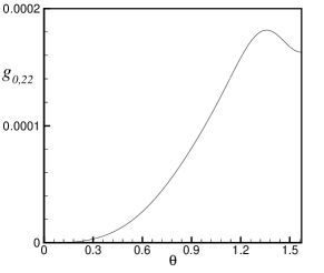
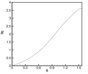
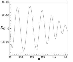
                          $(a)$ $(b)$ $(c)$

Figure 2: (a) The basis function $g_{0,22}(\theta)$ for $\gamma=0.7$ and $m=n=2$. (b) The residual function $R(\theta)$ when $\sigma(\theta)$ is approximated by ${\cal G}_{0}(v,w)$. (c) The global residual function $R_{G}(\theta)$.

As an example, we set $\gamma=0.7$ and follow the procedure mentioned above. We compute $a_{n}$ for different values of $N$ and increase $N$ until ${\cal J}$ attains its minimum ($\approx 10^{-12}$) and the accuracy of the numerical solutions is saturated. Our convergence condition is satisfied for $N=28$. We find that $\sigma_{N}(\theta)$ agrees with $\sigma(\theta)$ to an accuracy of $10^{-6}$, which is consistent with the minimum value of ${\cal J}$. The series expansion of ${\cal G}(w)$ is also convergent in the domain $0\leq w\leq w_{\rm max}$ where we have defined

$$w_{\rm max}=w_{+}(\frac{2}{4-\gamma},\theta=\frac{\pi}{2}),$$ (35)

so that $w_{\rm max}$ corresponds to the circular orbit in the equatorial plane. Figure 1a shows the variation of the residual function $R(\theta)=\sigma(\theta)-\sigma_{N}(\theta)$ versus $\theta$. The corresponding distribution function, which is a well-defined positive function, has been plotted versus $\overline{w}=w/w_{\rm max}$ and shown in Figure 1b. By studying the history of ${\cal J}$ versus $N$ (Figure 1c) it follows that the extremum of ${\cal J}$ is indeed a minimum. Furthermore, the envelope of the residual function is almost uniform, which indicates optimal fitting of $\sigma(\theta)$. Our numerical experiments show that the speed of convergence increases when $\gamma\rightarrow 0$.

An alternative method for the determination of the $a_{n}$ coefficients would be to expand $\sigma(\theta)$ and $g_{n}(\theta)$ in Fourier series, and to calculate $a_{n}$ by comparing the coefficients of the sine functions on both sides of (29). However, the evaluation of the Fourier coefficients considerably increases the required computational effort, and we have not followed this approach. Direct evaluation of $f(E,L_{z})$ by means of the HQ method is discussed in §4.1.

Our results show that, just as for the scale-free spheroids of Q95 and the scale-free power-law galaxies of Evans (1994), the scale-free ST models admit self-consistent $f(E,L_{z})$ distribution functions. In the former models the function $G(w)$ is monotonic, but for the ST models it has a maximum.

3.3 Distribution functions $f(E,L_{z},I_{3})$

Dejonghe & de Zeeuw (1988, hereafter DZ) constructed three-integral distribution functions for Kuzmin’s (1956) model using a generalized Fricke’s (1952) method. They expanded the given model density $\rho$ in terms of the potential $V$ and the polar cylindrical radius $\varpi=\sqrt{x^{2}+y^{2}}$, and wrote the distribution function $f$ as the sum of two parts: $f=f_{2}\!+\!f_{3}$. $f_{2}$ and $f_{3}$ are two- and three-integral distribution functions, respectively. One can integrate $f_{3}$ to obtain the corresponding density $\rho_{3}$, which is subtracted from $\rho$. The remaining density $\rho\!-\!\rho_{3}$ is then reproduced by $f_{2}$. DZ computed the coefficients of the Fricke expansion by direct comparison of the series representations for $\rho$ and the integral of $f$.

We can construct three-integral distribution functions by solving (24) for ${\cal G}(v,w)$ by means of a method developed by DZ for axisymmetric systems with Stäckel potentials. This can be considered as a perturbative approach in which one exploits the existence of two-integral distribution functions. We assume ${\cal G}$ has the form

$${\cal G}(v,w)={\cal G}_{0}(v,w)+{\cal G}_{1}(w).$$ (36)

Then, we choose a specific form for ${\cal G}_{0}(v,w)$ and compute the resulting density $\tilde{\sigma}(\theta)$. Subtracting $\tilde{\sigma}(\theta)$ from $\sigma(\theta)$ leaves a residual function $R(\theta)$. Finally, we determine the two-integral ${\cal G}_{1}(w)$ that is consistent with $R(\theta)$.

We first consider simple monomial forms for ${\cal G}_{0}$,

$${\cal G}_{0}(v,w)=a_{0,mn}v^{m}w^{n}.$$ (37)

Any combinations of (37) can also be chosen. By substituting (37) in the fundamental integral equation (24), and carrying out the integrations over $v$, $w$ and $u$, we find

$$\tilde{\sigma}(\theta)=a_{0,mn}g_{0,mn}(\theta).$$ (38)

The explicit expression for $g_{0,mn}(\theta)$ is (see Appendix A)

$$g_{0,mn}(\theta)\!\!\!\! = \!\!\!\!\sum_{i=0}^{m}\sum_{j=0}^{m-i}\!~{}\sum_{k=0}^{m-i-j}\sum_{l=0}^{i}{\scriptsize\left(\!\!\!\begin{array}[]{c}m\\ i\end{array}\!\!\!\right)}{\scriptsize\left(\!\!\!\begin{array}[]{c}m\!-\!i\\ j\end{array}\!\!\!\right)}{\scriptsize\left(\!\!\!\begin{array}[]{c}m\!-\!i\!-\!j\\ k\end{array}\!\!\!\right)}{\scriptsize\left(\!\!\!\begin{array}[]{c}i\\ l\end{array}\!\!\!\right)}$$

$$\!\!\!\!\times(-1)^{m-i-j-k+l}2^{i+k+\frac{n+1}{2}}{\rm B}(i+{\textstyle{1\over 2}},{\textstyle{1\over 2}})$$

$$\!\!\!\!\times{\rm B}\left({\textstyle{\gamma\over 2-\gamma}}\!+\!k\!+\!{\textstyle{m+n\over 2-\gamma}},1\!+\!i\!+\!j\!+\!{\textstyle{n+1\over 2}}\right)$$

$$\!\!\!\!\times\frac{{P_{1}(\theta)}^{m-i-2j+2k-\gamma k}{P_{2}(\theta)}^{n+1+2j}}{(1\!+\!n\!+\!2j\!+\!2l){P(\theta)}^{\frac{i}{2-\gamma}}},$$ (48)

where

$$P_{1}(\theta)=\frac{1+\cos\theta}{P(\theta)^{\frac{1}{2-\gamma}}},\qquad P_{2}(\theta)=\frac{\sin\theta}{P(\theta)^{\frac{1}{2-\gamma}}}.$$ (49)

We now calculate $R(\theta)=\sigma(\theta)-\tilde{\sigma}(\theta)$ and solve the following equation for ${\cal G}_{1}(w)$

$$R(\theta)=\pi\!\int\limits_{0}^{1}\!u^{2\gamma-3\over 2-\gamma}\,{\rm d}u\int\limits_{0}^{w_{+}(u,\theta)}\!\!\!\!{\cal G}_{1}(w){\rm d}w.$$ (50)

The solution of this equation for ${\cal G}_{1}(w)$ can be inserted in (36) to determine ${\cal G}(v,w)$. The performance of this technique depends on the initial choice of ${\cal G}_{0}(v,w)$.

As an example, we construct a three-integral distribution function for the same case discussed in §3.2. We take $\gamma=0.7$, $a_{0,22}=5000$ and assume $m=n=2$. This gives us the basis function $g_{0,22}(\theta)$ that is plotted in Figure 2a. The residual function of this step, $R(\theta)$, is displayed in Figure 2b. We now assume ${\cal G}_{1}(w)=\sum_{k=0}^{K}b_{k}w^{k}$ and find $K$ so that $R(\theta)$ is reproduced with the best available accuracy, i.e.,

$$R(\theta)\approx\tilde{R}(\theta)=\pi\sum_{k=0}^{K}b_{k}\int\limits_{0}^{1}\!u^{2\gamma-3\over 2-\gamma}\,{\rm d}u\int\limits_{0}^{w_{+}(u,\theta)}\!\!\!w^{k}{\rm d}w.$$ (51)

The constants $b_{k}$ are calculated by minimizing the objective function ${\cal J}_{1}=\int\nolimits_{0}^{\frac{\pi}{2}}\frac{1}{2}[R(\theta)-\tilde{R}(\theta)]^{2}{\rm d}\theta$ with respect to the variations of $b_{k}$. Numerical computation shows that ${\cal J}_{1}$ converges to a minimum of $5.3\times 10^{-12}$ by taking $K=15$. The global residual function, $R_{G}(\theta)=R(\theta)-\tilde{R}(\theta)$, is plotted in Figure 2c. The three-integral distribution function obtained from (36) is positive for all possible values of $u$ and $w$. The residual functions of the two- and three-integral distribution functions, displayed in Figures 1a and 2c, have similar behaviours. Their envelopes are nearly identical, and the maximum deviation from $\sigma(\theta)$ is approximately equal to the square root of the minimum value of the objective function, as expected. The minimum value of the objective function is the limit of available numerical accuracy.

4 ST models with central black holes

In the presence of a central black hole, i.e., when $M\not=0$ in equation (2), the ST models still have separable potentials but lose their scale-freeness. The construction of distribution functions by means of the series solutions of §3 becomes more complicated, even for the two-integral case. We overcome this problem by using the contour integral method of Hunter & Qian (1993).

4.1 Construction of $f(E,L_{z})$

The expressions for the density and potential of the ST models in cylindrical polar coordinates ($\varpi,\phi,z$) are given in equation (2.1). We consider the relative potential $\Psi=-V$ corresponding to the relative energy ${\cal E}=\Psi-\frac{1}{2}v^{2}$ (Binney & Tremaine 1987) with $v$ the modulus of the velocity vector.

The potential $\Psi$ can be split into $\Psi=\Psi_{\rm BH}+\Psi^{*}$ where $\Psi_{\rm BH}=GM/r$ and $\Psi^{*}$ is the potential induced by the density (2.1). The value of $L_{z}^{2}$ at a point $(\varpi,z)$ is obtained through

$$L_{z}^{2}=2\varpi^{2}\left[\Psi(\varpi^{2},z^{2})\!-\!{\cal E}\right]=-2\varpi_{c}^{4}\frac{{\rm d}\Psi(\varpi^{2},0)}{{\rm d}\varpi^{2}}|_{\varpi=\varpi_{c}},$$ (52)

where $\varpi_{c}$ is the radius of the circular orbit of energy ${\cal E}$ in the equatorial plane, which is obtained from

$${\cal E}=\Psi(\varpi_{c}^{2},0)+\varpi_{c}^{2}\frac{{\rm d}\Psi(\varpi^{2},0)}{{\rm d}\varpi^{2}}|_{\varpi=\varpi_{c}}.$$ (53)

At a fixed energy ${\cal E}$, $L_{z}$ takes its maximum value for $\varpi=\varpi_{c}$ and $z=0$. We denote this maximum by $L_{c}=L_{z}(\varpi_{c})$ and define $\overline{w}=L_{z}/L_{c}$, which is equal to $w/w_{\rm max}$ of equation (35). For the ST models equation (53) reads

$$(4-\gamma)\varpi_{c}^{3-\gamma}+{\cal E}\varpi_{c}-{\textstyle{1\over 2}}GM=0.$$ (54)

It is convenient to express (54) in terms of the dimensionless parameter $\zeta=[\Psi_{\rm BH}(\varpi_{c}^{2},0)/|\Psi^{*}(\varpi_{c}^{2},0)|]\geq 0$. Thus, we obtain $GM=2\zeta\varpi_{c}^{3-\gamma}$ and equation (54) is equivalent to

$$\varpi_{c}=[-{\cal E}/(4-\gamma-\zeta)]^{1\over 2-\gamma}.$$ (55)

It follows that $\zeta>1$ corresponds to the black hole sphere of influence, i.e., the region where the potential of the black hole dominates, and $0<\zeta<1$ outside this region.

       

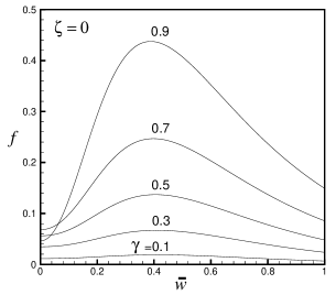
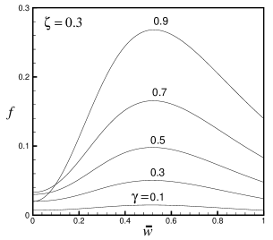
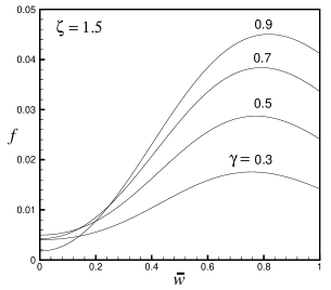
                        $(a)$ $(b)$ $(c)$

Figure 3: Physical distribution functions constructed for ST models using the HQ contour integral method. In all cases we have set ${\cal E}=-1$. Panel a with $\zeta=0$ corresponds to scale-free models in the absence of central black holes. Panel b corresponds to $\zeta=0.3$ outside the black hole sphere of influence. Panel c with $\zeta=1.5$ corresponds to the regions inside the black hole sphere of influence.

To apply the HQ method, we follow Q95 and express the density $\rho$ in terms of $\Psi$ and $\varpi^{2}$ as $\tilde{\rho}(\Psi,\varpi^{2})$ by eliminating $z^{2}$ between the expressions for the density and potential given in equation (2.1). The contour integral solution of HQ for axisymmetric models has the form

$$f({\cal E},L_{z}^{2})\!=\!\frac{1}{4\pi^{2}{\rm i}\sqrt{2}}\!\!\!\!\int\limits_{\Psi_{\infty}}^{[\Psi_{\rm env}({\cal E})+]}\!\!\!\!\!\!\!\tilde{\rho}_{11}\left[\wp,\frac{L_{z}^{2}}{2(\wp\!-\!{\cal E})}\right]\frac{{\rm d}\wp}{\sqrt{\wp\!-\!{\cal E}}},$$ (56)

which is evaluated in the complex $\wp$-plane. Following HQ and Q95, we use the subscript 1 to indicate a partial derivative with respect to the first argument of $\tilde{\rho}$. The symbol $[\Psi_{\rm env}({\cal E})+]$ indicates the contour of integration, which starts from $\Psi_{\infty}$ on the lower side of $\wp$-plane, crosses the real axis at $\Psi_{\rm env}({\cal E})$ and ends at $\Psi_{\infty}$ on the upper side of $\wp$-plane.

For the ST models we have $\Psi_{\infty}=-\infty$ and $\Psi_{\rm env}({\cal E})=\Psi(\varpi_{c}^{2},0)=2\varpi_{c}^{2-\gamma}(\zeta-1)$. The value of $\Psi_{\rm env}$ belongs to the interval $[\Psi_{\rm min},\Psi_{\rm max}]$ of physically achievable potentials on the real axis. To determine $\tilde{\rho}_{11}(\wp,\varpi^{2})$ we use the implicit relation

$$\tilde{\rho}_{11}(\wp,\varpi^{2})=\frac{\rho_{22}(\varpi^{2}\!,z^{2})}{[\Psi_{2}(\varpi^{2}\!,z^{2})]^{2}}\!-\!\frac{\rho_{2}(\varpi^{2}\!,z^{2})\Psi_{22}(\varpi^{2}\!,z^{2})}{[\Psi_{2}(\varpi^{2}\!,z^{2})]^{3}},$$ (57)

where each subscript 2 indicates partial differentiation with respect to the second argument, $z^{2}$. For a given pair $\{\wp,\varpi^{2}=L_{z}^{2}/[2(\wp-{\cal E})]\}$ on the contour of integration, the variable $z^{2}$ is supplied to (57) through solving the following nonlinear complex equation

$${\cal P}(z^{2})=\Psi\left[\frac{L_{z}^{2}}{2(\wp-{\cal E})},z^{2}\right]-\wp=0.$$ (58)

We use the modified Newton method for solving (58), and use the recursive formula

$$z^{2}_{n+1}=z^{2}_{n}+\frac{1}{2^{j}}\delta,\quad\delta=-\left[\frac{{\cal P}(z^{2})}{{\cal P}^{\prime}(z^{2})}\right]_{z^{2}=z^{2}_{n}},\quad^{\prime}\equiv\frac{\rm d}{{\rm d}z^{2}},$$ (59)

for obtaining the $(n+1)$th estimate of the root of ${\cal P}(z^{2})$. The coefficient $1/2^{j}$ allows for a univariate search along the gradient of ${\cal P}$ with the aim of taking the best step size towards the final answer. The integer exponent $j$ is determined through

$$j={\rm min}\{k:0\leq k\leq k_{\rm max},\|{\cal P}(z_{n}^{2}+\delta/2^{k})\|<\|{\cal P}(z_{n}^{2})\|\},$$ (60)

which guarantees a uniform and stable convergence. This algorithm fails if $k>k_{\rm max}$ and we have to change the initial choice $z_{0}^{2}$ for starting the recursion (59).

An appropriate contour is the one used by Q95, and defined by

$$\wp=\Psi_{\rm env}({\cal E})+l\left[1\!-\!\sec\left(\frac{\vartheta}{2}\right)\right]\!+\!{\rm i}h\sin\vartheta,\quad-\pi\leq\vartheta\leq\pi,$$ (61)

with $l$ and $h$ positive constants. The maximum width of the integration contour is controlled by $h$, while $l$ adjusts the location of the local maximum of the contour. The singularities (poles and branch points) of $\tilde{\rho}_{11}(\wp,\varpi^{2})$ play an important role in the integration along $[\Psi_{\rm env}({\cal E})+]$. Unfortunately, due to the implicit evaluation of $\tilde{\rho}_{11}(\wp,\varpi^{2})$, we have no clear idea about the possible singularities except for the branch point $\wp={\cal E}$ that corresponds to $\sqrt{\wp-{\cal E}}$ in the denominator of the integrand of (56). To gain a better sense, we changed the width of our contour and investigated the existence of singularities by monitoring the value of distribution function. We set $l=h=c|\Psi_{\rm env}({\cal E})|$ and evaluated the integral (56) for $c=0.2$, 0.5, 1, 5 and 10. The results were the same in all cases indicating that $\wp={\cal E}$ is the only singular point on the real axis and the integrand does not have any complex conjugate singularities. Our computations show that larger values of $c$ give more accurate results, and therefore we have used $c=5$ throughout.

We evaluate the contour integral (56) using a Gaussian quadrature. We carry out a change of independent variable as $\lambda=\cos\vartheta$ ($0\leq\vartheta\leq\pi$) and obtain

$${\rm d}\wp=\left[-l\frac{\sqrt{1\!-\!\lambda}}{\sqrt{2}(1\!+\!\lambda)}\!+\!{\rm i}h\lambda\right]\frac{-{\rm d}\lambda}{\sqrt{1\!-\!\lambda^{2}}},\quad-1\leq\lambda\leq+1,$$ (62)

which transforms (56) to

$$f({\cal E},L_{z}^{2})=\frac{(a\!+\!{\rm i}b)\!-\!(a\!-\!{\rm i}b)}{4\pi^{2}{\rm i}\sqrt{2}}=\frac{b}{2\pi^{2}\sqrt{2}},$$ (63)

where

$$a\!+\!{\rm i}b\!\!\! = \!\!\!\int\limits_{-1}^{+1}g(\lambda)\frac{{\rm d}\lambda}{\sqrt{1\!-\!\lambda^{2}}},$$

$$g(\lambda)\!\!\! = \!\!\!\left[-l\frac{\sqrt{1\!-\!\lambda}}{\sqrt{2}(1\!+\!\lambda)}\!+\!{\rm i}h\lambda\right]\tilde{\rho}_{11}\!\left(\wp(\lambda),\frac{L_{z}^{2}}{2[\wp(\lambda)\!-\!{\cal E}]}\right)\!.$$ (64)

Physical distribution functions correspond to $b\geq 0$. Assuming $W(\lambda)=1/\sqrt{1-\lambda^{2}}$ as the weight function, one can apply the $N$-point Gauss-Chebyshev quadrature formula (Press et al. 1992) and obtain

$$\int\limits_{-1}^{+1}g(\lambda)\frac{{\rm d}\lambda}{\sqrt{1-\lambda^{2}}}\approx\sum_{j=1}^{N}w_{j}g(\lambda_{j}),$$ (65)

where

$$w_{j}=\frac{\pi}{N},\quad\lambda_{j}=\cos\left[\frac{\pi(j\!-\!1/2)}{N}\right].$$ (66)

We solve (59) with an accuracy of $10^{-10}$ and increase $N$ until an accuracy of $10^{-8}$ is obtained in the integration of (4.1) using (65). For instance, we constructed distribution functions for ${\cal E}=-1$ and several values of $\zeta$ and $\gamma$. Figure 3 shows the results for $\zeta=0$, 0.3 and 1.5. Scale-free models without central black holes correspond to $\zeta=0$. As can be seen in Figure 3a, the graph of $\gamma=0.7$ is in agreement with ${\cal G}(\overline{w})$ of Figure 1b, which was constructed by means of the Fricke series.

By increasing the value of $\zeta$ (moving into the black hole sphere of influence), the maxima of $f(E,L_{z})$’s are shifted to the high-$L_{z}$ orbits (Figure 3). This means that sufficiently close to the central black hole, more nearly circular orbits are needed to maintain self-consistency in the ST models.

4.2 Distribution functions $f(E,L_{z},I_{3})$

         

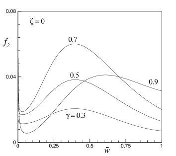
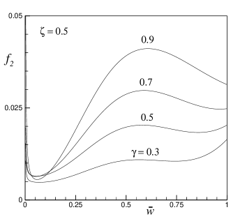
Figure 4: The two-integral $f_{2}$ part of the three-integral distribution functions of ST models for ${\cal E}=-2$. The left and right panels correspond to the scale-free ST models and ST models with central black holes, respectively. The value of $\zeta=0.5$ is relevant to the regions outside the black hole sphere of influence.

Three-integral distribution functions of ST models with central black holes can be derived as in §3 for the scale-free models. We again write $f(E,L_{z},I_{3})=f_{2}(E,L_{z})+\epsilon f_{3}(E,L_{z},I_{3})$, assume simple forms for $f_{3}$ and determine the density $\rho_{3}=\epsilon\int f_{3}{\rm d}^{3}{\boldmath v}$. We then subtract $\rho_{3}$ from $\rho$ and generate $f_{2}$ by the residual density $\rho_{2}=\rho-\rho_{3}$ using the method of HQ.

For example, we assume $f_{3}=E^{-4}I_{3}^{2}\delta(L_{z})$ where $\delta$ is the Dirac delta function. The corresponding density becomes (this is a consequence of eq. [12] for models with central black holes)

$$\rho_{3}\!\!\! = \!\!\!{\epsilon\pi\over 2\sqrt{\xi\eta}}\Big{[}{c_{1}^{2}+c_{2}^{2}\over V^{3}}+{3(\xi^{2}+\eta^{2})\over V}+{3(\eta c_{1}-\xi c_{2})\over V^{2}}$$ (67)

$$\qquad\qquad-{2\xi\eta\over V}+{2c_{1}c_{2}\over 3V^{3}}+{2(\eta c_{2}-\xi c_{1})\over V^{2}}\Big{]},$$

where

$$c_{1}=-2\eta^{3-\gamma}+GM,~{}~{}c_{2}=2\xi^{3-\gamma}-GM,$$ (68)

with $\xi$ and $\eta$ the parabolic coordinates. The potential function $V$ is given by (2.1). It is now straightforward to construct $f_{2}({\cal E},L_{z})$ from $\rho_{2}(\varpi^{2},z^{2})=\rho(\varpi^{2},z^{2})-\rho_{3}(\varpi^{2},z^{2})$ by following the procedure in §4.1. We have set $\epsilon=0.02$, ${\cal E}=-2$ and have constructed $f_{2}({\cal E},L_{z})\geq 0$ for several choices of $\gamma$ and $\zeta$. The results have been demonstrated in Figure 4. As this figure shows, $f_{2}({\cal E},L_{z})$ is oscillatory and steeply increases as $\overline{w}\rightarrow 0$. Our three-integral distribution functions exist both in the absence and in the presence of a central black hole for all values of $0<\gamma<1$.

5 Discussion

We have constructed two- and three-integral distribution functions for the cusped oblate models with central black holes introduced by Sridhar & Touma (1997a). We have computed $f(E,L_{z})$ for the case without a black hole by means of a Fricke (1952) series, and have confirmed the result by means of the contour integral method of Hunter & Qian (1993). The distribution function $f(E,L_{z})$ is of the form $E^{p}{\cal G}(\overline{w})$, with $p=-\frac{1}{2}-\frac{2}{2-\gamma}$ and $\overline{w}=L_{z}/L_{c}$ where $L_{c}(E)$ is the value of $L_{z}$ for the circular orbit of energy $E$. These distribution functions are non-negative for all values of the cusp slope $0<\gamma<1$, in agreement with the results obtained by Evans (1994) for scale-free power-law galaxies, and by Q95 for scale-free oblate spheroidal densities. By contrast to these other models, the function ${\cal G}(\overline{w})$ is not monotonic for the strongly dimpled shape of the ST models.

The ST models with a central black hole are not scale-free, but the HQ contour method shows that in this case again self-consistent $f(E,L_{z})$ exist. This makes the ST models significantly different from spheroidal cusps with central black holes, which do not admit a self-consistent $f(E,L_{z})$ when $\gamma<1/2$ (Q95; de Bruijne et al. 1996). We ascribe this difference to the dimpled shape of the ST models, as the density distribution can be considered as the weighted integral of two-integral components $\delta(E-E^{*})\delta(L_{z}-L_{z}^{*})$, each of which have toroidal shapes. This result is unlikely to depend on the separability of the ST models, or on the details of the orbit structure, as the computation of $f(E,L_{z})$ does not require any knowledge of the orbits, or indeed of the existence of an exact third integral. We speculate that the power-law galaxies of Evans (1994) can have a physical $f(E,L_{z})$ distribution function even when a central black hole is added. As the density $\rho$ of these models is a simple function of $\Psi$ and $\varpi^{2}$ (see Appendix D of Evans & de Zeeuw 1994), these distribution functions can be found by means of the HQ method following the procedure described in §4.1.

Nevertheless, the simple and exact form of $I_{3}$ in the ST models makes it possible to construct distribution functions $f(E,L_{z},I_{3})$ for these models, by means of a scheme introduced by Dejonghe & de Zeeuw (1988). These three-integral ST models have stars on the symmetric short-axis tube orbits as well as on pairs of reflected banana orbits (to ensure the symmetry with respect to the equatorial plane). The ST models have special shapes, but have a somewhat richer dynamical structure than, e.g., the oblate models with Stäckel potentials in spheroidal coordinates, which contain only one major orbit family, the short-axis tubes.

The two-dimensional versions of the ST models (Sridhar & Touma 1997b) are elongated discs, and no self-consistent distribution functions exist (Syer & Zhao 1998). The non-self-consistency of these models is related to the nature of the banana orbits that deposit much mass far from the major axis where the density is maximum. Although the meridional motions of the oblate ST models suffer this shortcoming too, their measure in the ($E,L_{z},I_{3}$) space is zero, and the short-axis tubes with $L_{z}\not=0$ have a sufficient variety of shapes to allow a range of self-consistent distribution functions.

Scale-free models with shallow cusps have mass distributions that diverge strongly at large radii, and infinite projected surface densities and stress tensors. Realistic models clearly require a radial profile that falls off more steeply at larger radii. Q95 and de Bruijne et al. (1996) have shown that at small and large radii the scale-free models provide insight into the dynamics of these more general models. The ST models similarly provide insight into the nature of galactic nuclei with a central black hole and a shallow luminosity cusp. In particular they indicate that the detailed shape of the surfaces of constant density may have a significant influence on the nature of the stellar velocity distribution.

6 acknowledgments

MAJ thanks the Sterrewacht Leiden for hospitality, and the Netherlands Research School for Astronomy NOVA for financial assistance.

Appendix A Determination of basis functions

The functions $g_{0,mn}(\theta)$ are given by

$$g_{0,mn}(\theta)\!=\!\int\limits_{0}^{1}\!\!u^{2\gamma-3\over 2-\gamma}{\rm d}u\!\!\!\!\int\limits_{0}^{w_{+}(u,\theta)}\!\!\!\!{\rm d}w\!\!\!\!\int\limits_{v_{-}(u,w,\theta)}^{v_{+}(u,w,\theta)}\frac{v^{m}w^{n}{\rm d}v}{\sqrt{[v\!-\!v_{-}][v_{+}\!-\!v]}},$$ (69)

where $v_{-}$ and $v_{+}$ are given in equation (3.1). Define the new variable

$$\mu=\frac{v-v_{-}}{v_{+}-v_{-}},\qquad 0\leq\mu\leq 1,$$ (70)

and rewrite (69) as

$$g_{0,mn}(\theta)\!=\!\!\int\limits_{0}^{1}\!\!u^{2\gamma-3\over 2-\gamma}{\rm d}u\!\!\!\!\!\int\limits_{0}^{w_{+}(u,\theta)}\!\!\!\!\!\!\!w^{n}{\rm d}w\!\!\int\limits_{0}^{1}\!\frac{[v_{-}\!+\!(v_{+}\!-\!v_{-})\mu]^{m}{\rm d}\mu}{\sqrt{\mu(1-\mu)}}.$$ (71)

The inner integral in (71) can be evaluated by writing out the binomial expansion for $[v_{-}+(v_{+}-v_{-})\mu]^{m}$, and using the definition of the beta-function. The result is

$$\sum_{i=0}^{m}{\scriptsize\left(\!\!\begin{array}[]{c}m\\ i\end{array}\!\!\right)}v_{-}^{m-i}(v_{+}\!-\!v_{-})^{i}{\rm B}(i\!+\!{\textstyle{1\over 2}},{\textstyle{1\over 2}}).$$ (72)

We now collect the $w$-dependent terms of $v_{-}$ and $v_{+}\!-\!v_{-}$ and write

$$v_{-}\!=\!v_{1}(u,\theta)\!+\!w^{2}\!v_{2}(u,\theta),\quad v_{+}\!-\!v_{-}\!=\!v_{3}(u,\theta)\!+\!w^{2}\!v_{4}(u,\theta),$$ (73)

where

$$v_{1}(u,\theta)\!\!\! = \!\!\!\frac{1+\cos\theta}{P(\theta)^{\frac{3-\gamma}{2-\gamma}}}[2u(1\!+\!\cos\theta)^{2-\gamma}\!-\!P(\theta)]u^{\frac{1}{2-\gamma}},$$

$$v_{2}(u,\theta)\!\!\! = \!\!\!u^{-\frac{1}{2-\gamma}}\frac{P(\theta)^{\frac{1}{2-\gamma}}}{2(1\!+\!\cos\theta)},$$

$$v_{3}(u,\theta)\!\!\! = \!\!\!2u^{\frac{1}{2-\gamma}}(1\!-\!u)P(\theta)^{-\frac{1}{2-\gamma}},$$

$$v_{4}(u,\theta)\!\!\! = \!\!\!-u^{-\frac{1}{2-\gamma}}\frac{P(\theta)^{\frac{1}{2-\gamma}}}{\sin^{2}\theta}.$$ (74)

By combining these results, and carrying out the integration over $w$, we obtain

$$g_{0,mn}(\theta)\!\!\! = \!\!\!\!\int\limits_{0}^{1}\!\!u^{2\gamma-3\over 2-\gamma}{\rm d}u\sum_{i=0}^{m}\sum_{j=0}^{m-i}\sum_{l=0}^{i}{\scriptsize\left(\!\!\begin{array}[]{c}m\\ i\end{array}\!\!\right)}{\scriptsize\left(\!\!\begin{array}[]{c}m\!-\!i\\ j\end{array}\!\!\right)}{\scriptsize\left(\!\!\begin{array}[]{c}i\\ l\end{array}\!\!\right)}$$

$$\!\!\!\!\times{\rm B}(i+{\textstyle{1\over 2}},{\textstyle{1\over 2}})v_{1}^{m-i-j}v_{2}^{j}v_{3}^{i-l}v_{4}^{l}$$

$$\!\!\!\times\frac{w_{+}(u,\theta)^{n+1+2j+2l}}{n+1+2j+2l}.$$ (82)

Finally, we replace $v_{1}^{m-i-j}$ with its binomial expansion, collect the $u$-dependent terms and then integrate over $u$. This gives us equation (3.3).

References

- [Binney & Tremaine 1987] Binney J., Tremaine S., 1987, Galactic Dynamics, Princeton University Press, Princeton
- [de Bruijne et al. 1996] de Bruijne J.H.J., van der Marel R.P., de Zeeuw P.T., 1996, MNRAS, 282, 909
- [Carollo et al. 1997] Carollo C.M., Franx M., Illingworth G.D., Forbes D., 1997, ApJ, 481, 710
- [Cretton et al. 1999] Cretton N., de Zeeuw P.T., van der Marel R.P., Rix H-W., 1999, ApJS, 124, 383
- [Cretton, Rix & de Zeeuw 2000] Cretton N., Rix H.-W., de Zeeuw P.T., 2000, ApJS, 536, 319
- [Dehnen & Gerhard 1994] Dehnen W., Gerhard O.E., 1994, MNRAS, 268, 1019
- [Dejonghe & de Zeeuw 1988] Dejonghe H., de Zeeuw P.T., 1988, ApJ, 333, 90 (DZ)
- [Evans 1994] Evans N.W., 1994, MNRAS, 267, 333
- [Evans & de Zeeuw 1994] Evans N.W., de Zeeuw P.T., 1994, MNRAS, 271, 202
- [Evans, Häfner & de Zeeuw 1997] Evans N.W., Häfner R.M., de Zeeuw P.T., 1997, MNRAS, 286, 315 (EHZ)
- [Fricke 1952] Fricke W., 1952, Astron. Nachr., 280, 193 (in German)
- [Gebhardt et al. 2000] Gebhardt K., Richstone D.O., Kormendy J., Lauer T.R., Ajhar E.A., Bender R., Dressler A., Faber S.M., Grillmair C., Magorrian J., Tremaine S.D., 2000, AJ, 119, 1157
- [Gradshteyn & Ryzhik 1980] Gradshteyn I.S., Ryzhik I.M., 1980, Table of Integrals, Series and Products, 4th edition, Academic Press, New York
- [Hunter & Qian 1993] Hunter C, Qian E.E., 1993, MNRAS, 262, 401 (HQ)
- [Jaffe et al. 1994] Jaffe W., Ford H.C., O’Connell R.W., van den Bosch F.C., Ferrarese L., 1994, AJ, 108, 1567
- [Jeans 1915] Jeans J.H., 1915, MNRAS, 76, 71
- [Kuzmin 1956] Kuzmin G.G., 1956, Astr. Zh., 33, 27
- [Lauer et al. 1995] Lauer T.R., Ajhar E, Byun Y.-I., Dressler A., Faber S.M., Grillmair C., Kormendy J., Richstone D.O., Tremaine S.D., 1995, AJ, 110, 2622
- [Levison & Richstone 1985] Levison H.F., Richstone D.O., 1985, ApJ, 295, 340
- [Lynden–Bell 1962] Lynden–Bell D., 1962a, MNRAS, 124, 1
- [Lynden–Bell 1962] Lynden–Bell D., 1962b, MNRAS, 124, 95
- [1] van der Marel R.P., Cretton N., de Zeeuw P.T., Rix H-W., 1998, ApJ 493, 613
- [Pars 1965] Pars L.A., 1965, A Treatise on Analytical Dynamics, John Wiley & Sons, Inc., New York
- [Press et al. 1992] Press W.H., Teukolsky S.A., Vetterling W.T., Flannery B.P., 1992, Numerical Recipes, Cambridge University Press, Cambridge
- [Qian et al. 1995] Qian E.E., de Zeeuw P.T., van der Marel R.P., Hunter C., 1995, MNRAS, 274, 602 (Q95)
- [Reddy 1986] Reddy J.N., 1986, Applied Functional Analysis and Variational Methods in Engineering, McGraw–Hill, New York
- [Rest et al. 2001] Rest A., van den Bosch F.C., Jaffe W., Tran H., Tsvetanov Z., Ford H.C., Davies J., Schafer J., 2001, AJ, 121, 2431
- [Richstone 1980] Richstone D.O., 1980, ApJ, 238, 103
- [Richstone 1984] Richstone D.O., 1984, ApJ, 281, 100
- [Richstone et al. 1999] Richstone D.O., et al., 1999, Nature, 395A, 14
- [Schwarzschild 1979] Schwarzschild M., 1979, ApJ, 232, 236
- [Sridhar & Touma 1997a] Sridhar S., Touma J., 1997a, MNRAS, 292, 657 (ST)
- [Sridhar & Touma 1997b] Sridhar S., Touma J., 1997b, MNRAS, 287, L1
- [Syer & Zhao 1998] Syer D., Zhao H.S., 1998, MNRAS, 296, 407
- [Toomre 1982] Toomre A., 1982, ApJ, 259, 535
- [de Zeeuw 1985] de Zeeuw P.T., 1985, MNRAS, 216, 273
- [de Zeeuw 2001] de Zeeuw P.T., 2001, in Black Holes in Binaries and Galactic Nuclei, eds L. Kaper, E.P.J. van den Heuvel & P.A. Woudt, ESO, 78
- [de Zeeuw, Peletier & Franx 1986] de Zeeuw P.T., Peletier R.F., Franx M., 1986, MNRAS, 221, 1001
- [de Zeeuw, Evans & Schwarzschild 1996] de Zeeuw P.T., Evans N.W., Schwarzschild M., 1996, MNRAS, 280, 903