A Catalogue and Analysis of X–ray luminosities of Early–type galaxies

Abstract

We present a catalogue of X–ray luminosities for 401 early–type galaxies, of which 136 are based on newly analysed ROSAT PSPC pointed observations. The remaining luminosities are taken from the literature and converted to a common energy band, spectral model and distance scale. Using this sample we fit the L_X:L_B relation for early–type galaxies and find a best fit slope for the catalogue of $\sim$2.2. We demonstrate the influence of group–dominant galaxies on the fit and present evidence that the relation is not well modeled by a single powerlaw fit. We also derive estimates of the contribution to galaxy X–ray luminosities from discrete sources and conclude that they provide L_dscr/L${}_{B}\simeq$29.5 erg s^-1 L${}_{B\odot}^{-1}$. We compare this result to luminosities from our catalogue. Lastly, we examine the influence of environment on galaxy X–ray luminosity and on the form of the L_X:L_B relation. We conclude that although environment undoubtedly affects the X-ray properties of individual galaxies, particularly those in the centres of groups and clusters, it does not change the nature of whole populations.

1 Introduction

One of the most surprising results from the Einstein observatory (launched in 1978) was the discovery of diffuse X–ray emission from early–type galaxies. Since then, many X–ray studies of galaxies have been published, ranging between detailed analyses of individual objects and large catalogues designed to shed light on their global properties. ? (FKT) produced one of the most extensive catalogues using Einstein data, observing 148 early–type galaxies and examining (among other things) the L_X:L_B relation for these objects. Other works in a similar vein include those of ?, a somewhat larger catalogue of Einstein data, ? and ? which use smaller samples based on ROSAT PSPC pointed observations, ? based on the ROSAT All–Sky Survey, and ? using ROSAT pointed data.

The largest of these catalogues, that of Beuing et al. , contains almost 300 galaxies, but most of these have exposure times of only a few hundred seconds. Catalogues based on pointed data have much longer exposures, but lack the coverage to be truly representative of the general population of early–type galaxies. The problem is exacerbated by the fact that most small and medium sized samples focus on the brightest objects, and pass over the fainter and less well studied galaxies. It can also be difficult to compare between catalogues, as each employs its own analysis procedure and presents results in its own particular format. For example, we have not used data from the sample of ? because the method used to convert count rates to fluxes is not based on a single spectral model, making it more difficult to correct luminosities from this catalogue to our own model and waveband.

Our intention in this paper is to provide a large general catalogue of X–ray luminosities for early–type galaxies. We have therefore calculated new X–ray luminosities for 136 galaxies, based on ROSAT PSPC data, and added a further 265 luminosities from previously published catalogues. All of the X–ray luminosities have been converted to a common format based on a reliable distance scale (assuming H₀ = 75 km s^-1 Mpc^-1) and correcting for differences in spectral fitting techniques and waveband. We use the resulting catalogue to study the X–ray properties of early–type galaxies, focusing in particular on the L_X:L_B relation and on the influence of environment.

In Section 2 we give details of our sample, and discuss our X–ray analysis of ROSAT data in Section 3. Section 4 covers the methods used to add data from the literature to our own results, and Section 5 briefly discusses the survival analysis techniques used to fit lines to censored data. In Section 7 we report the results of our line fits to the L_X:L_B relation, as well as giving an estimate of the contribution of discrete sources and examining the influence of galaxy environment. Section 8 is a discussion of some of our results and the conclusions we draw from them. Throughout the paper we normalise L_B using the solar luminosity in the B band, L_B⊙ = 5.2 $\times$ 10³² erg s^-1.

2 Sample selection

Our sample of early–type galaxies was selected from the Lyon–Meudon Extragalactic Data Archive (LEDA). This catalogue contains information on $\sim$100,000 galaxies, of which $\sim$40,000 have redshift and morphological data. Galaxies were selected using the following criteria:

• Morphological Type T $<-1.5$ (${\it i.e.\ }$ E, E–S0 and S0 galaxies)

• Virgo corrected recession velocity V $\leq$ 9,000 km s^-1

• Apparent Magnitude B${}_{T}\leq$ 13.5

The redshift and apparent magnitude restrictions were chosen in order to minimise the effects of incompleteness on our sample. The LEDA catalogue is known to be 90% complete at B_T = 14.5 (?), so our selection should be close to statistical completeness. The selection process produced $\sim$700 objects. We then cross–correlated this list with a list of public ROSAT PSPC pointings. Only pointings within 30^′ of the target were accepted as further off axis the PSPC point–spread function becomes large enough to make analysis problematic. This left us with 209 galaxies with X–ray data available.

3 Data Reduction and Spectral Fitting

Data reduction and analysis of the X–ray datasets were carried out using the asterix software package. Before the datasets can be used, various sources of contamination must be removed. Possible sources include charged particles and solar X–rays scattered into the telescope from the Earth’s atmosphere. Onboard instrumentation provides information which allows periods of high background to be identified. The master veto counter records the charged particle flux, and we have excluded all time periods during which the master veto rate exceeds 170 count s^-1. Solar contamination causes a significant overall increase in the X–ray event rate. To remove this contamination we excluded all times during which the event rate deviated from the mean by more than 2$\sigma$. This generally removes no more than a few percent of each dataset.

After this cleaning process each dataset is binned into a 3–dimensional (x, y, energy) data cube. Spectra or images can be extracted from such a cube by collapsing it along the axes. A model of the background is generated based on an annulus taken from this cube. We used annuli of width 0.1^∘, and inner radius 0.4^∘ where possible. In cases where this would place the annulus close to the source we moved the annulus, generally to r = 0.55^∘. To ensure that the background model is not biased by sources within the annulus, an iterative process was used to remove point sources of $>4.5\sigma$ significance. Occasionally the annulus lies over an area of diffuse emission, in which case we either remove that region by hand or move the annulus to an uncontaminated region. The only exception to this occurred in cases where the target galaxy was surrounded by group or cluster emission. In such cases the target is contaminated by group emission along the line of sight, increasing its apparent luminosity. To counter this we allowed the annulus to lie over the outer region of the group emission (unless prevented by large numbers of point sources), thereby removing at least a part of the contamination. The resulting background model was then used to produce a background-subtracted cube. Regions near the PSPC window support structure were removed from these images, as objects in those areas would have been partially obscured during the observation. The cube was further corrected for dead time and vignetting effects, and point sources were removed.

Examination of background subtracted images allowed us to locate each galaxy and produce a radial profile of its emission. This profile was used to determine the radius of the region from which a spectrum was extracted, with the cutoff radius taken at the point where the X–ray emission drops to the background level. We excluded 73 sources for which derived X–ray fluxes were unreliable at this stage. Many were too close to the support structure, or only had very poor quality data available. Others were found to be located close to bright X–ray sources. Galaxies in groups and clusters were only accepted if they stood out clearly above the general cluster emission. Point sources within the extraction region were not removed, as we considered these likely to be part of the galaxy emission. A spectrum of this region was then obtained by collapsing the cube along its x and y axes.

Galaxy spectra were fitted with a MEKAL hot plasma model (?; ?). Hydrogen absorption column densities were fixed at values determined from radio surveys (?), and temperature and metal abundance were fixed at 1 keV and 1 solar respectively. Fitting in this way provides a fairly crude measure of the bolometric X–ray flux, but allows all the galaxy spectra to be fitted by the same model, regardless of the quality of the data available.

Our choice of temperature and metallicity for these fits was influenced by our intention to combine our results with those of other studies. The catalogues of ? and ? both assume these values in their fits to early-type objects, although they use a Raymond & Smith (?) plasma model rather than the more accurate MEKAL model. There is a strong body of evidence showing that these parameters are representative of the majority of early-type galaxies. The recent study by ?, uses high quality ASCA observations to examine the gas metallicity in a number of X–ray luminous early-type galaxies. Taking into account probable errors in the modeling of the Fe–L spectral region, average metal abundances are found to be solar to within a factor of two, regardless of the plasma code used. Measured temperatures of early-type galaxies usually range between 0.2 and 1.3 keV (e.g. ?; ?), but finding an accurate average is hampered by the lack of high quality data.

The spectral representation we employ is clearly over–simplistic given that these objects are probably better fit by two component models (?). While such multi–temperature models should give more accurate measurements of halo gas temperatures, they require higher quality data, and have been used to date on only relatively small samples of bright galaxies. Single temperature 1 keV models are most likely to be poor descriptions of X-ray faint galaxies, which are expected to be dominated by emission from X-ray binaries (?). In these galaxies, emission is likely to be better represented by a high temperature bremsstrahlung model. If we assume that our lowest luminosity galaxies are actually better described by a 10 keV bremsstrahlung model, we find that we will have underestimated their bolometric luminosity by a factor of $\sim$2.

In total we fitted luminosities for 136 early–type galaxies, of which only 15 are upper limits. These form the core of our catalogue.

4 A Master Catalogue

Comparison of our new data with previously published catalogues was hampered by the different basic parameters used in these catalogues. The three catalogues we examined are those of ?, ? and ?. These use a range of models to fit the data, different wavebands, distances and blue luminosities. We have corrected for these differences by converting the catalogues to a common set of values, as used for our own results.

Where possible, we take our distances from ?. These are computed using the model of ? which accounts for the influence of the Great Attractor and Virgocentric flow. For galaxies not listed in Prugniel & Simien we used distances from LEDA, which are corrected only for Virgocentric motion. Similarly, we have calculated L_B for each object based where possible on the B_T values given in Prugniel & Simien. Where these are unavailable we use B_T, or in some cases m_B, from NED. Galaxies for which we have used m_B to calculate L_B are marked in the final catalogue, and in order to test their effect on our results we compared their distribution on an L_X:L_B graph with that of the rest of our catalogue. We found no significant difference between the two subsets. We therefore believe that these values provide us with a reasonably homogeneous and accurate set of distances and luminosities on which to base our study.

The three catalogues we wish to compare our results to each quote L_X in different wavebands. ? and ?, working with the Einstein IPC, quote luminosities in the 0.2–4.0 keV and 0.5–4.5 keV bands. ? choose a 0.64–2.36 keV band, as their work is based on relatively low signal to noise ROSAT PSPC All–Sky Survey data. To allow us to compare these with our luminosities we convert each to a pseudo–bolometric band. The spectral models available generally have limited energy range; for example, the Raymond & Smith model grid available on asterix covers the 0.088–17.25 keV range. However, we have assumed a typical galaxy temperature of 1 keV, as do the three other catalogues, so contributions to any model from outside the available range should be negligible. Using xspec (v11.0.1) we have tested this and find that changing the lower bound to 10 eV has no effect increases L_X by $\sim$6%, while changing the upper bound to 100 keV produces no measurable increase.

We also need to correct for different spectral models. For our analysis we have used the MEKAL model, as this is probably the most accurate generally available. However, both Beuing et al. and Fabbiano et al. use the Raymond & Smith model, and Roberts et al. use a simple bremsstrahlung model. Luckily, the choice of solar metallicity is common to all. Therefore, we calculated conversion factors between 1 keV, solar metallicity Raymond & Smith and bremsstrahlung models in the appropriate wavebands and our own MEKAL model in the pseudo–bolometric band. We then apply these corrections to the catalogues, bringing their luminosities into line with ours. The correction factors, including the effects of plasma code and conversion to bolometric luminosities, are shown in Table 1.

Catalogue	Correction Factor
	$\Delta$Log LX
Beuing et al.	+0.27
Fabbiano et al.	+0.15
Roberts et al.	+0.36

Table 1: Correction factors used to convert luminosities from Beuing et al. , Fabbiano et al. and Roberts et al. into our pseudo–bolometric band and MEKAL model.

To confirm that this process acts as intended, we compare L_X values for those galaxies which are listed in more than one catalogue. Plots of these comparisons are shown in Figure 1.

Figure 1: Comparisons of corrected bolometric L_X values from our PSPC pointed data and three other catalogues; a) Beuing et al. (1999), b) Fabbiano, Kim & Trinchieri (1992) and c) Roberts et al. (1991). Solid lines are best fits to the detections, excluding aberrant points as described in the text. Dotted lines show 1:1 relations between each pair of luminosities. All points, including those excluded from the fits, are marked as squares (detections) or arrows (upper limits).

In all three plots, a strong and fairly tight correlation is clear. In order to establish the relation between the three catalogues and our own points, we have fitted regression lines to the data. Galaxies actually detected in two catalogues should have very similar measured luminosities. However, the differences in data quality between the samples imply that upper limits may not be similar. We therefore fit the lines using detections only. We also expect a certain number of galaxies for which the measured luminosities disagree. There may be cases where the lower spatial resolution of the Einstein IPC or the small exposure times of the RASS observations allow confusion from nearby sources. Contamination from group or cluster emission is also likely to be dealt with differently in the different catalogues. To avoid bias from such cases we therefore exclude from our fits galaxies for which the luminosities disagree by more than a factor of $\sim$3. A search in NED revealed that all the galaxies thus excluded are either AGN (such as Cen A), surrounded by group or cluster emission (such as M86 or NGC 720) or lie near a much brighter companion galaxy (NGC 3605). Lastly, we also exclude the local group dwarf elliptical, M32, as it has a much lower luminosity than any of the other galaxies, and tends to drive the fitting process. With these galaxies excluded, we use the OLS bisector method to fit lines to the data. The slopes and intercepts are shown in Table 2.

Catalogue	Best Fit
	Slope (Error)	Intercept (Error)
Beuing et al.	0.971 ($\pm$0.031)	1.057 ($\pm$1.298)
FKT	1.014 ($\pm$0.028)	-0.672 ($\pm$1.160)
Roberts et al.	1.011 ($\pm$0.028)	-0.593 ($\pm$1.132)

Table 2: Comparison between galaxies from our PSPC pointed data and those from other samples.

The relations between the two Einstein–based catalogues and our own L_X values both have slopes close to unity, and small intercept values. We take this as an indication that the corrected catalogues are comparable. In the case of the Beuing et al. luminosities we find a slope of slightly less than unity, suggesting that their luminosities become systematically brighter than ours at high L_X. We believe this to be caused by a difference in analysis technique. Beuing et al. take source radii, as we do, as the radius at which the X–ray emission drops to the background level. However, when dealing with group–dominant galaxies they set the radius to include the group halo, whereas we attempt to use a radius at which the galaxy emission drops to the group level. This means that at high L_X, some of their luminosities include considerably more group emission than ours.

These relations show that our correction factors do indeed bring the catalogues into good agreement with one another. We do however recognize that there are likely to be factors we are unable to take into account, such as the use of different source extraction radii, and so we apply the relations defined in Table 2 as a further correction factor to the X–ray luminosities from the literature. In practice, it should be noted that the corrections are small (generally less than $\Delta$Log L_X = 0.1) and therefore have a minimal effect on the results presented in the rest of this paper.

5 Statistical Analysis

Before presenting the results of our new measurements, we first discuss the statistical techniques used to analyze the various correlations presented in this paper. Throughout this study we deal with data which contain both upper limits and detections. This is unavoidable when attempting to compile a large catalogue of galaxy X–ray luminosities. Many of the objects included only have serendipitous pointings available, and there are a number of faint galaxies which would require longer pointings to be detected.

To deal with data containing upper limits, we use the survival analysis tasks available in iraf. Survival analysis assumes that the censoring of the data is random – i.e. that the upper limits are unrelated to the true values of the parameter. In more detail, the assumption is made that for each upper limit, the distribution of detections below this value forms a reasonable model for the probability distribution of the true value associated with the upper limit. This assumption would be invalidated if, for example, sensitivity limits were systematically related to the true fluxes from sources – for example by observing known faint sources for longer in an attempt to detect them. In the case of our samples, we have upper limits representing galaxies over the majority of the range of L_X, and the detection limits are determined by exposure time, source distance, off axis angle and in some cases source environment. Most of the galaxies whose X–ray luminosities we have calculated based on ROSAT pointed data were not the target of the pointings used. This suggests that exposure time should be unrelated to the galaxy luminosity or distance. Similarly, luminosities taken from the Beuing et al. sample are based on exposures whose length is unrelated to any particular target. The situation is less clear in the case of the luminosities based on Einstein data, as more of these objects are likely to have been the target of the observation. However, for the great majority of galaxies, random censoring appears to be a fair assumption.

Three correlation tests are available in iraf; the generalized Kendall’s tau, generalized Spearman’s rho and Cox proportional hazard tests. Both the Kendall’s tau and Cox hazard tests are known to perform poorly when the data contains large numbers of tied values, and all three tasks function best on large datasets (?). Our samples are mainly large, in which case we use all three tests. We quote the least favourable result - i.e. the lowest significance found. In the few cases where a sample contains less than 30 objects we do not use the generalized Spearman’s rho test.

To fit lines to our samples we use two of the three linear regression tasks available. These are the expectation and maximization (EM) algorithm and the Buckley–James algorithm (BJ). The EM algorithm is a parametric test and assumes that the residuals to the fitted line follow a Gaussian distribution. The BJ method is non-parametric, using the Kaplan–Meier estimator for the residuals to calculate the regression, and therefore only requires the censoring distribution of the data about the line to be random. In almost all cases we find that these two methods agree reasonably well, and in most cases their results are nearly identical. However, in cases where the two methods are not in close agreement it should be noted that the BJ algorithm is probably the more reliable of the two, as it makes no assumption about the underlying distribution of the data. When using these tasks or the correlation tests, we take the uncensored parameter as the independent variable and the censored parameter as the dependent variable. The EM and BJ algorithms also produce values for the standard deviation about the regression, giving an estimate of the scatter in the relation.

The third linear regression task available to us is the Schmitt binning method. This technique can deal with upper limits on both axes, which allows allows a bisector fit to be carried out, based on fitting both y/x (y on x) and x/y regressions lines. However, the Schmitt algorithm is known to be unreliable when used with heavily censored data (?; ?), a result confirmed by the simulations reported in section 6. We therefore do not use Schmitt binning for our analysis.

To calculate means, we use the Kaplan–Meier estimator, which produces reliable results and error estimates except in cases where the lowest point in the data is an upper limit. When this occurs, the mean value derived tends to be underestimated. The estimator can also be used to effectively fit lines of fixed slope. For example, when fitting a line of slope unity to L_X:L_B relations, as the mean value of the L_X/L_B distribution is equal to the intercept of a slope unity line.

6 Tests of fitting accuracy

When attempting to determine the underlying relationship between two uncensored variables, an OLS bisector fit is likely to be the most reliable fitting method (?). For our censored data we have used the EM and BJ algorithms, which perform y on x regression. An alternative to these fits is to use the Schmitt binning method to perform y/x and x/y fits and then calculate a bisector of the two. We have carried out fits using this method, as described in ?, on various subsamples of our data. The slopes of these ‘Schmitt bisector’ fits are generally somewhat steeper than the EM and BJ fits, as might be expected. However, in many cases the slopes are very different from those found by the other two algorithms, and in a few cases a shallower slope is found. In order to test how well the three algorithms measure the underlying distribution of data, we have carried out a number of comparisons using simulated data.

We simulate datasets by using a random number generator to produce a set of data points, based on a predetermined straight line relation and range of x–values. We define a level of scatter, and points are shifted up or down by a random distance uniformly distributed within this range. To censor the data, we randomly select a number of data points and calculate a new y–axis value for each, corresponding to a detection threshold. If this new value is higher than the original, the data point is declared to be an upper limit at the new, higher value. The range of scatter of these detection thresholds is defined separately from the scatter in the data values, and both have been chosen to be comparable to that seen in our real dataset. Datasets containing the initial “detected” values (i.e. without any thresholding) are also produced, and these are fitted using a standard OLS bisector, as well as by the EM, BJ and Schmitt bisector methods.

As a test of the basic fitting properties of the four techniques, we simulated a line of slope 2, intercept 0, with x ranging between 0 and 10 and a scatter in the points of $\pm$0.5. We generated datasets containing 400, 200, 100 and 48 points, in which we censored 25, 50 and 75 per cent of the data. We also performed simulations involving 100 points with a larger scatter of $\pm$1. In all cases, the four techniques agreed well (within errors) with each other and with the original input slope. The Schmitt bisector generally produced slopes furthest from the OLS bisector slope. We conclude that all four techniques are capable of fitting a single line, though the survival analysis techniques may have problems in cases of large scatter.

However, our data set as a whole does not follow a single linear relationship. As can be seen in Figure 3, it is probably better described as a broken power law, with a shallow slope below L${}_{B}\simeq$10 and a steeper incline above. We therefore simulated a new dataset based on a broken power law similar to that indicated in our data (see Section 7.1), with a gradient of 1.0 over the range x=9.0-10.2, and gradient 2.5 over x=10.2-11.0. Scatter about each segment was set at $\pm$1 and each line was used to generate 150 data points, of which 75 were censored. The results of a variety of fits to this simulated dataset are shown in Figure 2.

The OLS bisector fit to this dataset gives a slope of $\sim$1.8, as does the Schmitt bisector which is offset downwards from the OLS bisector line. The EM and BJ algorithms both have slopes of $\sim$1.49. These results suggested that the Schmitt bisector does indeed behave, as expected, in a similar way to the OLS bisector fit, but that both are more influenced by the steeper line than the shallower. The y/x fits give consistently shallower slopes, but these may be more representative of the general spread of points.

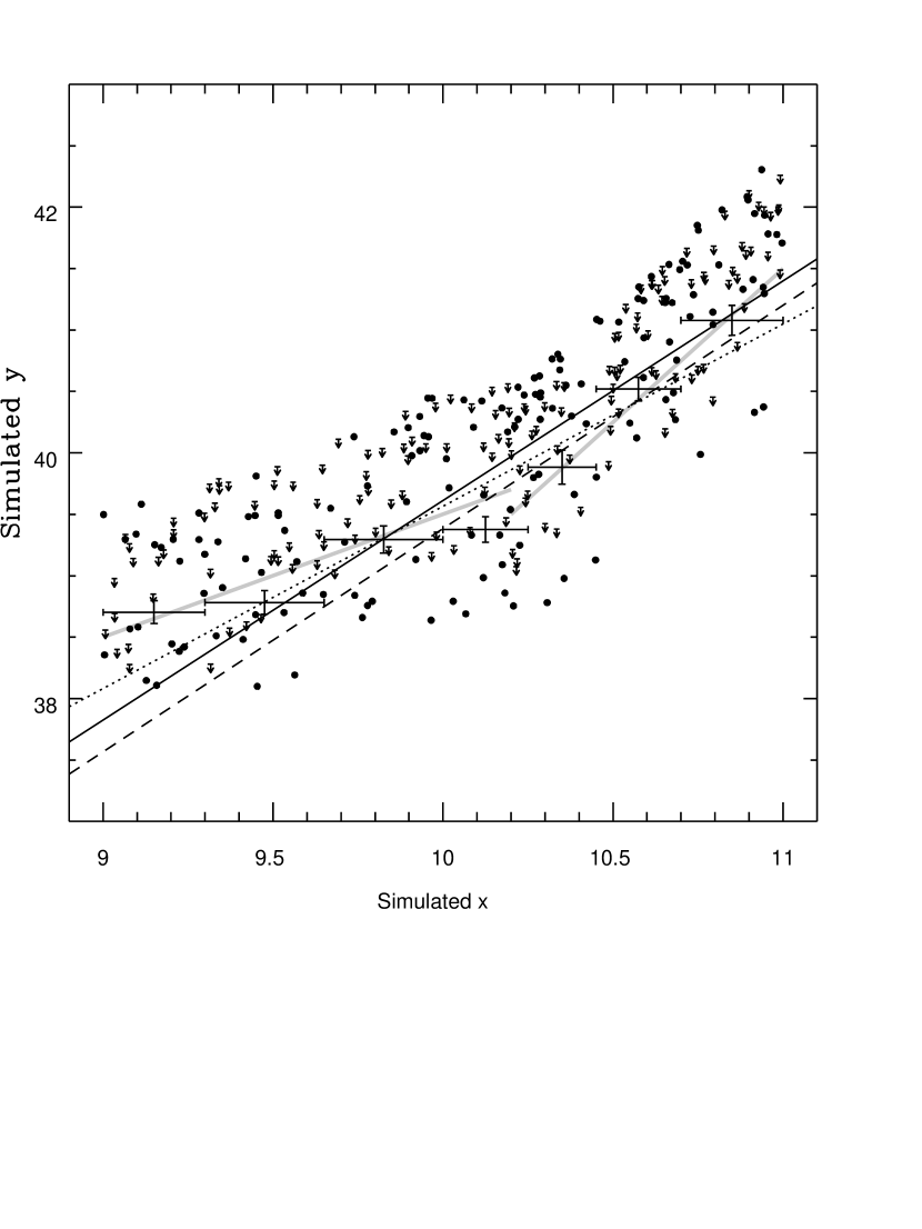
Figure 2: Simulated censored broken powerlaw data used to test alternative fitting methods. The solid line is an OLS bisector fit to the underlying, uncensored data, while the dashed line is a Schmitt bisector fit to the censored data. The dotted line represents the EM and BJ fits. The large crosses show the mean y value for the censored data with 1$\sigma$ errors in seven x axis bins, derived using the Kaplan–Meier estimator. The two solid grey lines show the original lines used to generate the data points.

To further test the quality of fit, we binned the data from the broken powerlaw simulation and used the Kaplan–Meier estimator to calculate the mean y value in each bin. The binned data are shown in Figure 2 and follow the original input lines fairly accurately. All four fit lines deviate from the binned data points at some point on the graph. Both bisector fits deviate quite strongly at low x and are probably better descriptors of the steeper high x points. The EM and BJ fits also deviate at low and high x values, but do a rather better job of describing the overall trend of the binned points across the whole range of x.

This result shows clearly that fitting a single line to data which is better described as the combination of two lines of different slopes will cause difficulties. The results from the single line simulations, when considered in conjunction with these results lead us to further conclude that for our data, which has a high degree of scatter and is unlikely to be described well by a single line, the Schmitt bisector should not be used. The EM and BJ algorithms appear likely to give reasonable estimates of mean trends, but binning the data should provide the most accurate picture of the underlying distribution.

7 Results

Having applied the corrections described in section 4, we add a total of 289 early–type galaxies from the three catalogues to our own. This gives a combined catalogue of 425 galaxies, listed in Table LABEL:Lxtab2. When galaxies are listed in more than one catalogue we choose the final L_X value using the following order of preference: our results, Beuing et al. (1999), Fabbiano et al. (1992), Roberts et al. (1991). Detections are always preferred to upper limits, regardless of source. The T–type listed in Table LABEL:Lxtab2 is taken from LEDA. The catalogue contains 24 galaxies which are listed in previous studies as early–type, but which have LEDA T–types $\geq$–1.5. We exclude these late–type objects from further consideration.

7.1 The L_X:L_B Relation for Early Type Galaxies

We have plotted Log L_X against L_B for the catalogue in Figure 3. AGN (taken from ?) and cluster central galaxies are likely to have anomalously high X–ray luminosities and are marked on the plot. Excluding these objects and dwarf galaxies (L${}_{B}<$ 10⁹ L_B⊙ ), which are unlikely to be massive enough to retain a halo of X–ray gas, leaves 359 early–type galaxies of which 184 have X–ray upper limits. The tests described in Section 5 show a correlation of $>$99.99% significance. The best fit line from the expectation and maximization (EM) algorithm is:

$$Log\thinspace L_{X}=(2.17\pm 0.11)\thinspace Log\thinspace L_{B}+(17.98\pm 1.12)$$ (1)

and from the Buckley–James (BJ) algorithm:

$$Log\thinspace L_{X}=(2.28\pm 0.12)\thinspace Log\thinspace L_{B}+16.80$$ (2)

The standard deviations about the two regression lines are $\sigma_{\sc em}$=0.69 and $\sigma_{\sc bj}$=0.68 respectively.

Figure 3: Log L_X vs Log L_B for our full catalogue of 401 early-type galaxies. Triangles are cluster central galaxies, stars AGN and circles all other detections. The lines shown are the best fit line to the early–type galaxies excluding AGN, BCGs and dwarfs (solid line), the best fit to the galaxies excluding all questionable objects (dashed line), and an estimate of the discrete source contribution taken from Ciotti et al. (1991).

These values are in fairly good agreement with a number of previous estimates (?; ?; ?), but differ from those of ? who found a slope of $\sim$2.7 using a small sample of optically bright galaxies.

X–ray emission from discrete sources is expected to produce a lower bound to the distribution of galaxies in Figure 3. We discuss the question of discrete source emission in detail in Section 7.3, but at this stage we note that our points are reasonably consistent with the estimate of discrete source emission made by ?.

Previous work with group galaxies (?) has shown that the properties of central dominant group galaxies are substantially different from those of normal group members and field galaxies. The X-ray luminosity of these dominant galaxies is in fact more closely correlated with the properties of the group as a whole than with the optical luminosity of the galaxy (?). Temperature profiles of X-ray bright groups suggest that these objects are at the centres of group cooling flows, which explains their overluminosity compared to non-central galaxies. The Brown & Bregman sample contains a large number of group–dominant galaxies (?), which may account for the high slope of their best fit L_X:L_B relation.

Group–dominant galaxies can be identified by their position at the centre of the group X–ray halo. Unfortunately, since part of our catalogue is drawn from the literature, we are unable to carry out identifications in this way. However, group–dominant galaxies are usually the most massive and luminous object in the group. In order to remove any bias produced by these dominant galaxies, we excluded all brightest group galaxies (BGGs) and then fitted the remaining data. The majority of BGGs are selected using the catalogue of groups by ?. However, 48 of our galaxies lie beyond the Garcia redshift limit (5,500 km s^-1), and in these cases we are forced to identify BGGs using other catalogues. Using NED, we were able to check each galaxy for membership of the catalogues of ?, ?, ? and ?. As White et al. do not list the BGG of each group, we have identified them based on the apparent magnitudes given in NED.

In order to check for other objects which might bias the fits, we also used NED to check all galaxies with log L_X/L_B $>$ 31.5 for unusual properties. A surprising number of these objects show potential problems. For example, we found several probable AGN not identified in ? (e.g. NGC 3998, NGC 4203, NGC 7465). Excluding all BCGs, BGGs, AGN and dwarf galaxies, leaves a total of 270 objects. Fitting L_X:L_B for this reduced sample lowers the slope of the best fit lines significantly, to 1.98$\pm$0.13 (EM) or 2.17$\pm$0.15 (BJ), with $\sigma_{\sc em}$=0.69 and $\sigma_{\sc bj}$=0.70. This change demonstrates the influence of BGGs on the L_X:L_B relation.

As a final precaution we also fit a very conservative subsample, from which we have removed not only all AGN, BCGs, BGGs and dwarf galaxies, but also all objects which lie at a distance $>$70 Mpc, to avoid including misclassified galaxies. We also remove the anomalous galaxies NGC 5102 and NGC 4782 from this conservative subsample. NGC 4782 has an unusually high L_B, and the B magnitude given for it in Prugniel & Simien (1996) disagrees with those in LEDA and NED by $>$1 magnitude. NGC 5102 is a relatively small E–S0 galaxy (Log L_B = 9.29 L_⊙) with an exceptionally low X–ray luminosity (Log L_X = 38.03 erg s^-1). It is thought to have undergone an episode of star formation a few 10⁸ years ago (?). Although during and shortly after the starburst we might expect to observe an enhanced L_X compared to L_B (?), galactic wind models predict that the starburst can remove all gas from the galaxy, leaving it significantly underluminous until the halo is rebuilt (?; ?). The B–band luminosity will also be enhanced by the population of young stars produced by the starburst, making the position of such an object on an L_X:L_B plot even more aberrant.

Removing all of these objects reduces our dataset to 246 galaxies, of which 159 have X–ray upper limits. This lowers the slope of the best fit lines considerably, to 1.63$\pm$0.14 (EM) and 1.94$\pm$0.17 (BJ), with $\sigma_{\sc em}$=0.60 and $\sigma_{\sc bj}$=0.62. The difference in results between the two fitting methods in this case is large, particularly as the 1$\sigma$ error regions do not overlap. As mentioned in Section 5, the only difference between the two techniques is the assumed underlying distribution of points. As the EM method assumes the distribution to be normal, we tested the distribution of detections (87 points) for normality, using the algorithm AS 248 (?; ?) which provides several measures of goodness of fit. These tests showed that the detected points were normally distributed about the best fit line at 50-60% significance. This is not a strong confirmation of the normality of the data, but is also not poor enough to rule out a normal distribution.

It is notable that the agreement between the two fitting algorithms worsens as the fraction of upper limits in the data increases. Our complete catalogue has $\sim$50%, and the fits are in reasonable agreement, whereas our conservative subsample has $\sim$65% upper limits and shows poor agreement. ? simulate fits to datasets containing 30 points, of which $\frac{2}{3}$ are upper limits, and produce acceptable results, but their data does not appear to have as large a degree of scatter as ours. It seems likely that our conservative subsample is rather poorly constrained, and is perhaps not well modeled by a normal distribution. This suggests that the BJ method is the more reliable in this case.

Figure 4: Our catalogued data L_X and L_B data with mean L_X values for eight bins. Open circles are BGGs, triangles are BCGs, stars are AGN, filled circles are detected normal galaxies and arrows are upper limits. The large crosses show the mean L_X in eight bins, calculated using the Kaplan–Meier estimator and excluding AGN, BCGs, BGGs, dwarfs, galaxies at distances $>$70 Mpc, NGC 5102 and NGC 4782. The diamond shows the mean L_X in the lowest bin, corrected to remove the expected contribution from discrete sources (see Section 7.3.6). The dotted lines are EM (shallower) and BJ (steeper) fits to the same data.

Even excluding BGGs, there is some evidence of a change in the slope of the L_X:L_B relation above L${}_{B}\simeq$10 L_B⊙. To see how this apparent change in slope affects our fits, we binned the very conservative sample and calculated the mean L_X in each bin. These are plotted in Figure 4. The bins clearly follow a general trend, but at low L_B, the gradient becomes shallower. We also defined a new sample of data which excludes AGN, BGGs, BCGs, galaxies with distances $>$70 Mpc L${}_{B}<$10, NGC 5102 and NGC 4782. This sample should have had most points which are likely to bias the fit removed, and with L${}_{B}>$10 it should model the steeper section of the relation. EM and BJ fits to this sample give slopes of 1.96$\pm$0.25 and 2.28$\pm$0.29 respectively, with standard deviations about the fits in both cases of $\sigma$=0.58. Both fits seem to do a reasonably good job of matching the binned data points at L${}_{B}>$10, with the EM fit being slightly closer to the points at high and low L_B.

7.2 Potential sources of bias

Our catalogue is made up of X–ray luminosities which can be split in to three main categories; those which we have calculated based on pointed ROSAT PSPC data, those which are based on ROSAT All–Sky Survey data, and those which are based on pointed Einstein IPC data. Clearly it is important to examine possible biases which may arise from this combination of data.

? have carried out a ROSAT study of 52 galaxies with optical fine structure. In order to check the accuracy of their own analysis of PSPC pointed data, they compare their own count rates with those of ?. For the majority of their sample both analyses are in agreement, but they note that in three cases the count rates differ by more than a factor of two. The objects concerned are NGC 7626, in the Pegasus I cluster, NGC 3226 which has an X–ray bright neighbour, and NGC 4203 which is close to an unrelated X–ray source. The inclusion of the neighbouring sources in the Beuing et al. analysis for the latter two cases is caused by the short exposure times (typically $\sim$400 s) of RASS observations. Although extraction radii for detected galaxies were based on surface brightness profiles, low numbers of counts may cause close pairs of sources to be blurred together, appearing as a single object.

A similar but perhaps more serious problem occurs in cases where the target galaxy is surrounded by X–ray emission from a group or cluster halo. In these cases, Beuing et al. calculate luminosities for those galaxies which clearly stand out from the emission or are at the center of emission which is reasonably symmetric around them. Galaxies which stand out from the background emission may have overestimated luminosities, owing to the inclusion of emission from that part of the group/cluster halo lying along the line of sight. However, this is true of most luminosity estimates for galaxies in such environments, and as the galaxy clearly stands out against its surroundings, it seems fair to assume that its own emission dominates. On the other hand, it seems likely that galaxies in the centres of groups and clusters will have seriously over-estimated luminosities, due to the inclusion of the majority of the surrounding halo emission. Beuing et al. exclude cluster dominant galaxies from their fitting, but not group–dominant galaxies, which may steepen the slope of their L_X:L_B relation.

Despite the corrections described in Section 4, we are almost certainly including some data from Beuing et al. which are biased by inclusion of extraneous sources or group emission. However, we perform fits which exclude BGGs, and may therefore expect to remove the majority of the most biased points. It is also worth noting that Beuing et al. calculate upper limits on X–ray luminosity using a fixed aperture 6 optical half–light radii in diameter, and do not use upper limits for galaxies embedded in bright cluster emission.

Luminosities calculated from Einstein data are generally based on considerably larger numbers of counts than those taken from the RASS. They should therefore be somewhat less likely to suffer from the problems described above. Unfortunately the poorer spatial resolution of the IPC compared to the PSPC makes confusion of close sources more likely, particularly if the sources are relatively faint. Our comparisons in Section 4 show that there is no major systematic offset, but there are still likely to be individual galaxies which have been over–estimated.

In our own analysis of PSPC pointed data we have attempted to avoid these problems where possible. Confusion between close sources should be minimal, as we work with considerably larger numbers of counts. We have attempted to remove at least a part of any contaminating group or cluster emission where possible, reducing the degree to which group and cluster gas biases the L_X:L_B relation. However, without two dimensional fitting of the surface brightness profile of the group and galaxy it is not possible to completely remove this contamination, so we must expect to over–estimate some of the luminosities.

Figure 5: Log L_X vs Log L_B for our sample of 136 early–type galaxies from ROSAT PSPC pointed observations. Filled squares are early–type galaxies, triangles represent cluster central galaxies and stars AGN. The solid line is our best fit to the data, excluding AGN, dwarfs and cluster central galaxies. The dashed line is the Beuing et al. best fit relation.

In order to examine our data for possible biasing effects we have fitted an L_X:L_B relation for a subset of the catalogue, made up of those galaxies whose X–ray luminosities are the product of our own analysis of PSPC data. Figure 5 shows a plot of Log L_X vs Log L_B for this sample. For the complete subset, the statistical tests described in section 5 show a probability $>$99.99% that a correlation exists, and give slopes of 1.73$\pm$0.12 (EM) and 1.71$\pm$0.13 (BJ) respectively. The standard deviations about the two regressions are $\sigma_{\sc em}$=0.74 and $\sigma_{\sc bj}$=0.69.

As discussed in Section 7.1, fitting a line to the complete sample does not provide a good estimate of the true L_X:L_B relation for the sample, as there are a number of unusual objects included. Removing cluster central galaxies, AGN and dwarf galaxies steepens the slope to 1.81$\pm$0.15 (EM) or 1.79$\pm$0.15 (BJ), with $\sigma_{\sc em}$=0.61 and $\sigma_{\sc bj}$=0.59. The EM fit is shown as the solid line in Figure 5.

For comparison the L_X:L_B relation of ?, which has a slope of 2.23$\pm$0.13, is shown. It is clear that the Beuing et al. line is not a particularly good fit to the data. However, our fitted slopes are similar to the slope found by ? for their sample of elliptical galaxies observed with Einstein. We believe that these differences in slope are caused by the different analysis strategies adopted for the three samples, and that the steeper slope of the Beuing et al. data may be caused by cases of over–estimation of L_X, as discussed above.

7.3 The Discrete Source Contribution

The X-ray emission from early-type galaxies is thought to be produced by a combination of sources. These can be generalized into two categories; hot gas and discrete sources. Discrete sources (e.g. X-ray binaries, individual stars, globular clusters) are essentially stellar in origin and so the total X-ray luminosity from these sources should scale with L_B. This can seen in the L_X:L_B relation of Beuing et al. (1999), which at low L_B agrees well with discrete source estimates with slope unity. However, the normalization of these discrete source estimates is not well defined – those quoted in Beuing vary over at least an order of magnitude, and only the highest is ruled out by that data set.

Most previous estimates of the discrete source contribution to L_X (hereafter L_dscr ) are based on a small number of relatively nearby objects. For example, ? base their estimates on Einstein observations of M31, ? use Centaurus A, while ? use M31 and NGC 1291. Estimates based on early-type galaxies are rare, as it is difficult to separate a discrete source component from the overall emission. One simple method to avoid this problem is employed by ?, who fit a slope unity line to the lower envelope of data from ?. This gives an estimate of log(L_dscr /L_B) = 29.45 erg s^-1 (using our pseudo-bolometric bandpass and model). This value has been shown to be a good estimate of the lower bound of the Beuing et al. sample, and is also a reasonably good match to our data. However, this does not necessarily imply that the value is a good estimate of the mean L_dscr . To produce more accurate estimates we need either a large sample of data from late-type galaxies which have little or no hot gas emission, or much more detailed spectral studies of early-type objects.

7.3.1 X-ray emission from late-type galaxies

Late-type galaxies are known to be sources of X-ray emission, though not of the same magnitude as elliptical and S0 galaxies (e.g. ?). Early studies (?) showed that there is a strong correlation between the X-ray and optical emission, giving rise to an L_X:L_B relation similar to that observed for early-type galaxies. However, in late-type galaxies this relation has a much shallower slope than in early-types. Most studies find this slope to be $\mathrel{\hbox to0.0pt{\lower 3.0pt\hbox{$\sim$}\hss}\raise 2.0pt\hbox{$>$}}$ 1.

The most common explanation for this relation is that the X-ray emission observed is produced mainly by X-ray binaries and hot stars. As these sources are stellar in origin, their numbers should be directly related to the optical luminosity of the galaxy, and the L_X:L_B relation for spirals should have a slope of $\simeq$ 1. Emission from other sources, such as hot gas, may not be so directly linked to stellar populations. If spiral galaxies contain significant amounts of hot gas as well as discrete sources, we would expect to see an L_X:L_B relation for with a slope $\geq$ 1.

Detailed spectral studies of the X-ray emission from nearby spiral galaxies (e.g. ?; ?; ?) have shown that such a hot gas component is present in some cases. Using a large sample of galaxies observed with Einstein, ? showed that this ISM component was mainly associated with early–type (Sa) spirals, and that there was a succession of spectral properties with morphology. Elliptical and E/S0 galaxies were mainly dominated by gaseous emission, S0 galaxies had a somewhat harder spectrum, Sa spirals were harder still with the hard component dominating, and late–type spirals showed little sign of a hot ISM. This points toward the hot gas being associated with the bulge of the galaxy; Sb and Sc galaxies have small bulges and little or no hot gas, whereas ellipticals are essentially all bulge, and have large gaseous halos.

More recent studies have confirmed the lack of significant halos around spiral galaxies. ? used ROSAT observations of three massive edge-on spiral galaxies to look for large scale extended emission predicted by galaxy formation models to arise as hot gas cools to form the galaxies’ disks. They found no evidence for X–ray halos of the extent seen around early–type galaxies. Studies of diffuse emission within or near spiral galaxies suggest that hot gas does not extend far beyond the stellar body of the galaxy except in the case of starburst galaxies (?). We have avoided all such galaxies, as the contribution to the X–ray emission from active star–formation and the associated galactic winds would seriously affect our results.

To define an L_dscr:L_B relation for spirals we tried two approaches. The first was to search the literature for attempts to separate gaseous and discrete emission in spiral galaxies. The second was to obtain a large sample of spiral galaxies observed in X-rays and split this into subsamples by morphological type. The hierarchical merger scenario implies that galaxies with small bulges should have minimal X-ray emission from hot gas, so there should be a trend for a lower and less steep L_X:L_B relation for later-type spirals.

7.3.2 Nearby spiral galaxies sample

We have collected L_X values for 13 spirals, and normalised them to bolometric luminosities. The following list gives details of these sources:

• Nine galaxies from ?. The objects chosen are those which are not listed as starburst galaxies in the paper, NGC 55, NGC 247, NGC 300, NGC 598, NGC 1291, NGC 3628, NGC 3628, NGC 4258 and NGC 5055. The X-ray luminosities given are for emission from the galaxies after any resolved point sources had been removed.

• M83, from ?. The $L_{X}$ value given is for the harder of two diffuse emission components fitted, thought to represent unresolved discrete sources in the disk and bulge. Resolved point sources were removed before fitting.

• Centaurus A (NGC 5128), from ?. The $L_{X}$ value given is for the 5 keV component of a two temperature Raymond & Smith plasma model fitted to the diffuse emission from the galaxy. Regions contaminated by the nucleus and associated jet were removed, but some point source emission was included.

• NGC 4631, from ?. The value used is that given for a soft (0.2-0.8 keV) component associated with the disk of this galaxy.

• The bulge of M31, from ?.

Figure 6: Plot of $L_{X}$ vs $L_{B}$ for a sample of nearby late-type galaxies. Solid triangles represent data from Read, Ponman & Strickland (1997), the square M83, the cross NGC 4631, the star Centaurus A, and the circle the bulge of M31. The solid line is the best fit slope unity line, with the other lines showing estimates of $L_{dscr}$ from the literature. The dotted line is the estimate of Ciotti et al. (1991), the short dashed is taken from Forman et al. (1985) and the long dashed is from Canizares et al. (1987)

In most of the cases listed above, we have selected the component of emission which is most likely to represent the discrete sources in each galaxy, and excluded components corresponding to gaseous emission. However, we have also excluded a number of resolved point sources, which could be a part of the discrete source population. To be resolved by the instruments used in these studies, the point sources must be highly luminous. At worst, this suggests that they might be AGN or bright transient sources. At best they could be unusually powerful LMXBs, or possibly black hole binaries. We have decided to exclude these sources to avoid the possibility of contaminating the sample with emission from objects which are not part of the population in which we are interested.

The results are shown in Figure 6. iraf survival analysis tasks were then used to fit lines to these points, both with a fixed slope of unity and with the slope allowed to vary. Using the Kaplan-Meier estimator, we found the intercept of the slope unity line to be 29.56 $\pm$ 0.13. Fitting of a variable slope line with the EM algorithm gave a slope of 1.21 $\pm$ 0.15 and an intercept of 27.51 $\pm$ 1.44. The fixed slope line is plotted on Figure 6, as well as three estimates of discrete source emission taken from ?, ? and ?. Our line agrees within errors with that of Ciotti et al. .

7.3.3 Morphologically defined samples

Group	N	Unit slope	Variable slope
		intercept	slope	intercept
Sa	90	30.59 $\pm$ 0.11	2.14 $\pm$ 0.31	19.07 $\pm$ 3.07
Sb	74	30.22 $\pm$ 0.09	1.14 $\pm$ 0.29	28.77 $\pm$ 2.90
Sc	98	30.12 $\pm$ 0.06	1.38 $\pm$ 0.16	16.35 $\pm$ 1.60

Table 3: Slopes and intercepts of four morphological subsamples selected from Fabbiano, Kim & Trinchieri (1992)

Figure 7: Plot of $L_{X}$ vs $L_{B}$ for morphological subsets of late-type galaxies from Fabbiano, Kim & Trinchieri (1992). Circles are Sa, squares Sb, crosses Sc, and triangles Sd and Irregular galaxies. Upper limits from all classes are shown as arrows. The solid line is the same as that shown in Figure 6, while the dotted lines are slope unity fits to the four subclasses. The dashed line corresponds to the slope unity fit to the data below Log L_B = 9.9 L_B⊙ . See text for further details.

Working with the large spiral sample of Fabbiano et al. (1992) we define three morphological subsets; Sa, Sb and Sc. Results from fits to the L_X:L_B properties of these subsets with fixed (unity) and variable slopes are shown in Figure 7 and listed in Table 3. It can be seen that there is a distinct difference between the earlier-type spirals in group 1, and the later types in groups 2 and 3. Therefore, it seems that these results support the idea that X-ray gas luminosity is correlated with bulge size, though the effect is not large.

As a check of this result we have also carried out fits to samples of spiral galaxies taken from the catalogue of ?. This catalogue, although it contains a larger number of galaxies than that of Fabbiano et al. , is dominated by upper limits and uses an average of three spectral models to convert count rates to fluxes. We have not therefore converted it to our waveband and model, but have instead simply compared general trends in the results with those we find using the Fabbiano et al. data. Fitting lines of unit slope to Sa, Sb and Sc subsamples we find a similar trend in relative normalisation; the Sa sample has an intercept significantly above either of the other subsets.

The line fits to the Fabbiano et al. data and the data values themselves can be seen in Figure 7. For comparison the fit to the nearby spiral data discussed above is also shown. It is clear that even the lowest of the fits to the ? data is considerably higher than that to the nearby galaxies, presumably owing to the removal of point sources and (in some cases) gaseous emission from the nearby spiral data.

In Figure 7, it can be seen that as $L_{B}$ increases, the data points for all the subclasses diverge more and more from the slope unity lines. We therefore decided to split the sample into two new subsets. These are the low luminosity (Log $L_{B}\leq$ 9.9 L_B⊙ ) and high luminosity (Log $L_{B}>$ 9.9 L_B⊙ ) subsets. Line fits for each are shown in Table 4.

Group	N	Unit slope	Variable slope
		intercept	slope	intercept
Low $L_{B}$	115	30.15 $\pm$ 0.06	1.01 $\pm$ 0.13	30.34 $\pm$ 1.18
High $L_{B}$	164		2.03 $\pm$ 0.38	20.13 $\pm$ 3.93

Table 4: Slopes and intercepts for the high (Log $L_{B}>$ 9.9 L_B⊙ ) and low luminosity subsets.

These figures show clearly that there is a large difference in the L_X:L_B relation for low and high luminosity spirals. The high $L_{B}$ subset has a slope similar to that found for elliptical galaxies, while the low $L_{B}$ sample slope is very close to 1. The slope unity fit to the low L_B sample is shown in Figure 7 as a dashed line.

7.3.4 L_dscr from early-type galaxies

In order to directly measure L_dscr from early-type galaxies, it is necessary to distinguish between emission from hot gas and the contribution of the discrete source population. Whereas X-ray bright galaxies are usually fit using a single component MEKAL or Raymond & Smith model with kT$\sim$1 keV, X-ray faint galaxies have been shown to be better fit by two component models (?; ?). These consist of a high temperature (kT $\sim$ 10 keV) component generally associated with X-ray binaries and a low temperature component with kT$\sim$0.2 keV. A number of possible sources for this low temperature component have been suggested (e.g. ?), but LMXBs again seem to be the most likely source (?; ?). The advent of Chandra has made it possible to resolve significant numbers of point sources in nearby galaxies. Observations of NGC 4697 (?) and NGC 1553 (?) reveal considerable numbers of point sources with hard spectra. Blanton et al. show that, at least in the case of NGC 1553, the emission from resolved point sources is best fit using a model which includes a low temperature component. From the Blanton et al. results we estimate that the total flux from discrete sources, excluding the AGN, is 8.58$\times$10^-13 erg s^-1 cm^-2 in the 0.3-10 keV band. Using our distance and L_B for NGC 1553 gives L_dscr = 29.44. As we do not have the exact details of the Blanton et al. best fit model, we cannot convert this to our own model and waveband, but any correction should be small, as the Chandra waveband extends to much higher energies than that of Einstein or ROSAT. Assuming a 20% conversion factor produces L_dscr = 29.52, very similar to our other estimates. However, both NGC 1553 and NGC 4697 have low X–ray luminosities, and relying purely on the lowest luminosity galaxies for measurements of L_dscr may be unwise. ? note that small fluctuations in the discrete source populations in these objects could cause a large degree of scatter in L_X, as their total X-ray luminosities are small. This is confirmed by comparison of the luminosity functions of the point source populations of four galaxies observed by Chandra (?). Theses show differences in L_dscr of a factor $\geq$ 4 between the galaxies. Clearly estimates based on large samples are likely to be more reliable.

With high quality ASCA data, it is possible to fit high luminosity galaxies using both a 1 keV gaseous halo and a high temperature discrete component (e.g. ?). The most recent study of this sort (?) fits a 10 keV bremsstrahlung model to 27 galaxies, excluding those which show signs of harboring low luminosity AGN, producing a value of Log L_dscr = 29.41 L_B⊙ (converted to our passband and model). Given the quality of the data used, this is probably the most reliable value available from studies of elliptical galaxies. Its only drawback is that it does not take into account the effects of a low temperature component in LMXB emission. Such a component is unlikely to be detected by ASCA, which has a relatively low collecting area and poor spectral capabilities below 1 keV. Assuming the Chandra observation of Sarazin et al. to be representative, we expect that the effects of such a component would be strongly affected by hydrogen column, but would only increase L_dscr by up to a factor of two (i.e. 0.3 dex).

One other interesting method of estimating the discrete contribution is that of ?. This involves fitting the surface brightness profiles of seven elliptical galaxies, representing the hot gas component with a King profile and the discrete sources with a de Vaucouleurs r^1/4 profile. Using the fitted normalisation of the de Vaucouleurs component, Brown and Bregman find a median best fit Log L_dscr/L_B = 28.51 erg s^-1, with a 99% upper limit of Log L_dscr/L_B = 29.21 erg s^-1. Although this method should in principle be able to produce similar results to 2-component spectral fitting, these values are somewhat lower than those found by other methods. This may be a product of the small size of the sample, or of assuming circular symmetry to allow 1-dimensional profile fitting. It also remains to be established how well the discrete X–ray source population is modeled by a de Vaucouleurs profile which fits the optical profile. The excellent spatial resolution of Chandra should allow this question to be answered in the near future.

7.3.5 Summary

Possible choices for Log $L_{dscr}$ (in units of erg s^-1 L${}_{B\odot}^{-1}$) are then as follows:

• Nearby late-type galaxies sample intercept = 29.56 $\pm$ 0.13

• Sc galaxy sample intercept = 30.12 $\pm$ 0.06

• Low $L_{B}$ sample intercept = 30.15 $\pm$ 0.11

• ? estimate = 29.45

• ? hard component = 29.41

• ? Chandra estimate from NGC 1553 $\simeq$ 29.52

• ? 99% upper limit $\leq$ 29.21

These values are compared with our data in Figure 8.

Figure 8: Plot of our early-type galaxies with L_dscr estimates marked. The dotted lines represent the seven estimates listed in section 7.3.5, and the solid line marks L_X/L_B = 29.5. Point symbols are the same as those in Figure 3.

As the two higher values are derived from samples in which $L_{X}$ may include emission from gas and bright point sources, they do not seem reliable options. The Brown & Bregman value is considerably lower than the other estimates, particularly as it is an upper limit. The values from Ciotti et al. , Matsushita et al. , Blanton et al. and the nearby galaxies sample agree within errors, and would seem to be a reasonable choices. A value of Log L_dscr = 29.5 L_B⊙ lies between the four and is close to being the average. This value is marked in Figure 8 as a solid line. This value cannot be considered to be a “hard” lower limit; as the plot shows, a number of our data points lie below this line. For dwarf galaxies (L${}_{B}<$ 9.0), we may expect to see quite large variations in L_X. Each dwarf needs only a small number of LMXBs to produce the expected luminosity of 10^36-38 erg s^-1, so minor variations in population can produce large changes in integrated luminosity. In larger galaxies this statistical variation is less important, but some degree of scatter in L_X may be expected to result from factors such as different galaxy evolutionary histories. It is also worth noting that, as discussed in Section 3, we expect to underestimate the luminosity of galaxies whose X–ray emission is primarily from LMXBs, owing to our assumption of a 1 keV MEKAL model. With the exception of NGC 5102, all our detected non-dwarf galaxies are within a factor of three of our L_dscr estimate. All upper limits are also within this range, although NGC 1375 has a luminosity of almost exactly L_dscr /3. Given the factor of two expected from underestimation of L_X in these galaxies and the factor of four variation in L_dscr found by ?, we conclude that our data are consistent with our estimate of L_dscr , within the expected errors.

7.3.6 The L_X-L_dscr:L_B relation

Using our value of L_dscr, we can now examine how removing stellar emission affects our L_X:L_B relation. This should provide us with a more accurate measure of the relation between the luminosity of the galaxies’ gaseous halos and their optical luminosity. As we expect a real variation of a factor $\sim$4 in L_dscr between galaxies, we cannot simply subtract the mean expected L_dscr from all values of L_X. To do so would produce extremely low values of L_X for galaxies with total luminosities similar to L_dscr, strongly biasing any fits. We have therefore removed all galaxies which have L_X values within a factor of 4 of L_dscr , and subtracted the mean expected L_dscr from the remainder. Excluding AGN, BCGs and galaxies with L${}_{B}<$9 L_B⊙ , this leaves us with a total sample of 257 points, of which 136 are upper limits. Fitting this dataset we find slopes of 2.03$\pm$0.1 (EM) and 2.00$\pm$0.13 (BJ). The standard deviation about the regression line is 0.58 in both cases. If we further exclude galaxies to form a very conservative sample as described in Section 7.1, the slopes of the fits are lowered to 1.63$\pm$0.13 (EM) and 1.60$\pm$0.14 (BJ). The data and these fits are shown in Figure 9.

Figure 9: Log [L_X-L_dscr] against L_B for all galaxies in our main catalogue with Log L_X/L${}_{B}>$30.1 (4$\times$L_dscr). Open circles are BGGs, triangles and BCGs, stars are AGN, filled circles are normal detected galaxies and arrows are upper limits. The Solid line is the best fit to the sample excluding AGN, BCGs and dwarf galaxies. The dashed line is the best fit to a very conservative sample which also excludes BGGs, galaxies at a distance$>$ 70 Mpc, NGC 5102 and NGC 4782. The dotted line shows our estimate of L_dscr=29.5.

These fits are very similar to those produced by fitting the L_X:L_B relation to the sample as a whole (see Table 6 for a comparison). This is to be expected, as although L_dscr is comparable to the L_X/L_B values of some of the galaxies, the majority have luminosities inconsistent with X-ray emission from discrete sources alone. As these galaxies are dominated by gas emission, subtraction of the discrete source contribution has little effect on their overall luminosity. In order to test the robustness of this result, we also fitted samples based on excluding galaxies with X–ray luminosities within factors of 2 and of 6 of L_dscr. In the latter case, the slopes are slightly steeper when excluding AGN, BCGs and dwarfs ($\sim$1.9) and slightly shallower for the more conservative sample ($\sim$1.5). This is likely to be an effect of the smaller number of data points (136) and larger numbers of upper limits (97). However, when we use a factor of 2 the slopes are less well defined; for the sample excluding AGN, BCGs and dwarfs we find slopes of 2.14$\pm$0.11 (EM) and 2.31$\pm$0.14 (BJ). For the conservative sample, the slopes are again shallower, but still not in good agreement, with values of 1.61$\pm$0.14 and 2.08$\pm$0.19. As these datasets are similar in size to the corresponding samples used in fitting the L_X:L_B relation, this scatter is probably a product of the underlying distribution rather than an effect of subtracting L_dscr .

Figure 4 (Section 6) shows that at low L_B the slope of the L_X:L_B relation breaks and becomes shallower. A possible explanation for this is that the observed X–ray luminosities are the result of a combination of emission from discrete sources and hot gas. A break in the slope would then suggest that the shallower section is dominated by the discrete sources while the steeper section is more influenced by gas emission. Similarly, the lowest binned point in Figure 4 will have an X–ray luminosity dominated by discrete source emission, whereas the fit lines will describe the relation for gas emission. If this is the case, then subtracting the mean value of L_dscr expected for the lowest bin should move the point downwards, into agreement with the line fits. We calculate that the mean value of L${}_{X}^{gas}$ for the bin is L_X-L_dscr=38.96, which is in marginal agreement, at the high L_B end of the bin, with the EM fit. However, it is important to note that we expect to underestimate the luminosities of galaxies which are dominated by discrete source emission by a factor of $\sim$2, due to our use of an inappropriately soft spectral model. This may mean that the mean L_X value calculated for the bin is also underestimated. It may also be important to take into account the expected variations in L_dscr between galaxies. Although we expect a scatter of a factor of $\sim$4, some of the galaxies in this low L_B bin have very low X–ray luminosities, which could be significantly affected by small differences in the number of X-ray binaries they contain. We cannot therefore be certain, on the basis of the data presented here, that the break in the relation is caused by the change from gas dominated to discrete source dominated galaxies.

7.4 Environmental Dependence of L_X/L_B 

Although there are several suggested mechanisms by which the environment of a galaxy can affect its X–ray properties, the actual role these effects play is unclear. The observational evidence is conflicting and often difficult to interpret.

? found that for a sample of early–type galaxies studied by Einstein, galaxies with Log L_X/L_B $<$ 30 (erg s^-1 L${}_{B\odot}^{-1}$) had $\sim$ 50% more neighbours than X–ray bright galaxies. They attributed this to ram–pressure stripping, which would be expected to reduce L_X more in higher density environments. An opposite view was presented by ?, who found that L_X/L_B increased with environmental density. Their explanation was that for the majority of galaxies (with the possible exception of those in the densest environments) ram–pressure stripping is a less important effect than the stifling of galactic winds by a surrounding intra–group or –cluster medium. In this model, the IGM/ICM encloses the galaxy, increasing the gas density of its halo and therefore its X–ray luminosity.

Brown & Bregman (1999) claimed an environmental dependence based on a correlation between L_X/L_B and Tully density parameter $\rho$ (?) for their 34 galaxies. However, ? show that group–dominant galaxies, of which there are several in Brown & Bregman’s sample, often have X–ray luminosities which are governed by the properties of the group rather than the galaxy. Their high luminosities are more likely to be caused by a group cooling flow than by a large galaxy halo. Once these objects are removed from consideration, the correlation between L_X/L_B and $\rho$ is weakened to a $\sim$1.5$\sigma$ effect (?).

Our larger sample of galaxies gives us the opportunity to study this correlation over a wide range of L_X, L_B and environmental density. If Figure 10 we therefore plot L_X/L_B against $\rho$ for 196 of our galaxies listed in the Tully catalogue.

Figure 10: Plot of normalized X–ray luminosity against environmental density. Open squares are field galaxies, filled circles non–central group galaxies, crossed circles BGGs, asterisks cluster galaxies and arrows upper limits of all types.

Galaxies in this plot are subdivided into group, cluster and field samples. Cluster membership was based on the ? and ? catalogues while group membership was taken from ?. In total, this gives 50 cluster galaxies and 113 group galaxies. Brightest Group Galaxies were also taken from ? and it is important to remember that these objects are only brightest optically, not necessarily the dominant galaxy at the center of the group or group X–ray halo. However, we believe that the majority are actually group–dominant galaxies. The group subset contains 37 BGGs. The remaining 33 galaxies not listed in the cluster or group catalogues were assumed to lie in the field. This is probably the weakest classification and is likely to be contaminated to some extent with galaxies at the edges of clusters and groups.

The plot shows no obvious trend, but to check for weak correlations we used the statistical tests described in section 5. No trend was found in the sample as a whole, nor in any of the subsamples. We also calculated mean L_X/L_B values for each of the subsamples, excluding all AGN, BCGs and dwarf galaxies. These values are shown in table 5. The field, group and cluster subsamples have similar mean values, while the BGG subsample has a slightly larger mean L_X/L_B , as might be expected from the previous results.

Subset	mean LX/LB	Error
Cluster	29.733∗	$\pm$0.094
Field	29.548	$\pm$0.196
Group (total)	29.908	$\pm$0.066
Group (non-BGG)	29.719∗	$\pm$0.065
Group (BGG)	29.977	$\pm$0.096

Table 5: Mean L_X/L_B values for the environmental subsamples shown in Figure 10. Values marked by an asterisk may be slightly biased as the lowest value in the sample was an upper limit.

Figure 11: Plot of L_X/L_B against $\rho$ for non–BGG galaxies from the sample of Brown & Bregman (1999). L_X/L_B values are from our catalogue, $rho$ values are from Tully (1988). The dotted line is the best fit to the data, and the large crosses are mean values for the three bins described in the text. Other symbols are the same as in Figure 10.

The lack of a general correlation is surprising, as the previous studies suggest we should find at least a weak trend. As we are using the same method as Brown & Bregman, we decided to check for a correlation in their sample of galaxies using our own X–ray luminosities. These data (excluding galaxies identified as BGGs in Helsdon et al. ) are plotted in Figure 11.

Although there is more scatter in L_X/L_B than seen in Brown & Bregman’s plot, a trend for increasing L_X/L_B with environmental density is clear. Statistical tests show the correlation to be at least 97% (2.5$\sigma$) significant, with a best fit slope of 0.78 (EM) or 0.75 (BJ). Binning the data in the same ranges as used by Brown & Bregman and Helsdon et al. produces the three large crosses in the plot. These also clearly show a trend, despite the fact that the centre and right hand crosses are likely to be biased downwards as the lowest points in these bins are upper limits.

As the trend is seen in this sample of galaxies but not in our more general catalogue, it seems likely that it is a product of the sample selection process. Brown & Bregman’s sample is composed of the 34 optically brightest galaxies chosen from ?, excluding AGN and dwarf galaxies. The selection of bright galaxies has one clear effect; more than half of their galaxies are BGGs, likely to have unusually high X–ray luminosities. Of the remaining galaxies, three are found in the field, six are in groups and five in clusters. Of the cluster galaxies, the two most X–ray luminous are NGC 1404, a large E1 galaxy in the Fornax cluster, and NGC 4552 (M89), one of the large ellipticals in the Virgo cluster. The high L_X values of these two galaxies and the low L_X value of NGC 5102 have a strong influence on the fitted slope. Indeed, when using our data, their removal eliminates the correlation altogether. NGC 4552 is known to be a Seyfert 2 (?), and therefore its X–ray luminosity is likely to be misleading. NGC 1404 may also be an unusual case, as it lies within the X–ray envelope of NGC 1399 and may be interacting with it (?). As mentioned in Section 7, NGC 5102 is a recent ($\sim$400 Myr) post–starburst galaxy and has a population of young blue stars (?) which may have ‘artificially’ raised its B band luminosity.

7.5 The L_X:L_B relation in different Environments

In order to gain another viewpoint on the relation between environment and X–ray luminosity, we decided to examine the L_X:L_B relation in field, group and cluster environments. We split the sample as described above, but no longer limited ourselves to galaxies listed in the Tully catalogue. The sample therefore included all galaxies within 5,500 km s^-1 (the limit of the Garcia (1993) group catalogue). The resultant fits are shown in Table 6, along with the fits to the field, group and cluster sets. In each case we have removed cluster central galaxies, AGN, dwarf galaxies and galaxies at distances $>$70 Mpc before fitting. The cluster sample contains 57 objects (of which 36 are upper limits), the field sample 76 objects (55 upper limits) and the group sample 185 objects (85 upper limits). Separating BGGs from the group sample gives a non–BGG sample of 116 objects (69 upper limits) and a BGG sample of 69 objects (16 upper limits).

Subset	Fit	Slope (Error)	Intercept (Error)
Combined	EM	1.63 ($\pm$0.14)	23.38 ($\pm$1.41)
	BJ	1.94 ($\pm$0.17)	20.13
LX-Ldscr	EM	1.63 ($\pm$0.13)	23.70 ($\pm$1.36)
	BJ	1.60 ($\pm$0.14)	24.11
Cluster	EM	1.77 ($\pm$0.27)	21.91 ($\pm$2.71)
	BJ	1.77 ($\pm$0.29)	21.93
Field	EM	1.62 ($\pm$0.23)	23.58 ($\pm$2.40)
	BJ	1.61 ($\pm$0.26)	23.61
Group (total)	EM	1.92 ($\pm$0.13)	20.56 ($\pm$1.39)
	BJ	1.90 ($\pm$0.16)	20.73
Group (non–BGG)	EM	1.62 ($\pm$0.14)	23.57 ($\pm$1.39)
	BJ	1.59 ($\pm$0.16)	23.85
Group (BGG)	EM	2.58 ($\pm$0.36)	13.60 ($\pm$3.76)
	BJ	2.57 ($\pm$0.40)	13.71

Table 6: Best fit L_X:L_B lines for galaxies in field, group and cluster environments. All subsets exclude AGN, BCGs, dwarf galaxies and galaxies at distances $>$ 70 Mpc. The Combined values for the complete sample excluding BGGs, and the best fits to the L_X-L_dscr:L_B relation are shown for comparison.

Figure 12 shows plots of the cluster, field and group data with best fit lines. In terms of L_B, it is notable that although the field and group sets cover a similar range, there are very few optically faint cluster galaxies. This is likely to be caused by the difficulty of observing small, X–ray faint galaxies in an X–ray bright ICM. In the field no such problem occurs, and many groups are faint enough to allow such small objects to be observed. Both group and cluster data show a number of highly X–ray luminous objects, probably giant ellipticals and group or cluster dominant galaxies at the centers of large X–ray halos. In the field, only one galaxy (NGC 6482) has Log L${}_{X}>$ 42 erg s^-1 and the high end of the L_X:L_B line is sparsely populated. Comparing L_X:L_B slopes shows a similar trend, with the BGG sample producing the steepest slope, then cluster galaxies, non–BGGs and lastly field galaxies with the shallowest relation. The slope of the BGG sample is similar, within errors, to that of the best fit line to the Brown & Bregman sample.

It is interesting to note that the slopes for the field, cluster and non-BGG group samples are all similar, within errors. Table 6 also shows the fits to the catalogue as a whole, excluding AGN, BCGs, BGGs, dwarfs and galaxies at distances $>$ 70 Mpc. The EM fit to this supersample agrees with the fits to the three subsamples, and the BJ fit has overlapping errors with the field and cluster subsamples. This suggests that the L_X:L_B relation may be similar for the different environmental subsets when biasing objects are excluded. To further investigate this similarity, we have fitted fixed slope lines to the field, group, cluster and combined subsets described above. As the EM and BJ algorithms find slopes of 1.63 and 1.94 for the combined subset, we use these values. Table 7 shows the resulting intercepts and errors, calculated using the Kaplan-Meier estimator. In both cases, the intercepts for the field, cluster and non-BGG group subsets agree within errors, and also agree with the intercept of the combined subset, whilst the BGG intercept is markedly higher. Our results suggest, then, that with the exception of BGGs, early-type galaxies have a universal mean L_X:L_B relation which is unaffected by environment.

	Slope = 1.63	Slope = 1.94
Subset	Intercept (Error)	Intercept (Error)
Combined	23.446 ($\pm$0.048)	20.252 ($\pm$0.054)
Cluster	23.384 ($\pm$0.091)	20.253 ($\pm$0.096)
Field	23.446 ($\pm$0.109)	20.247 ($\pm$0.126)
Group (total)	23.457 ($\pm$0.049)	20.323 ($\pm$0.051)
Group (non-BGG)	23.473 ($\pm$0.062)	20.266 ($\pm$0.069)
Group (BGG)	23.667 ($\pm$0.083)	20.401 ($\pm$0.081)

Table 7: Best fit intercepts to L_X:L_B relations with fixed slopes as shown in the table. All values are calculated using the Kaplan-Meier estimator. All subsamples exclude AGN, BCGs, dwarf galaxies and galaxies at distances $>$ 70 Mpc. The Combined subset also excludes BGGs.

Figure 12: L_X/L_B data for a) field, b) group and c) cluster subsets. In each plot the solid line represents the best fit to the sample, excluding AGN (marked as stars), BCGs (marked as triangles), dwarfs and galaxies at distances $>$70 Mpc. In Fig. b, open circles represent BGGs, and the two dashed lines show fits to the BGGs (long dashes) and to the remaining sample with BGGs excluded (short dashes). The dotted line in Figures b and c represents the EM fit to the complete catalogue with exclusions as above. This fit is not shown in Figure a, as it is indistinguishable from the fit to the subsample.

8 Discussion and Conclusions

8.1 The L_X:L_B Relation for Early–type Galaxies

The slope of the L_X:L_B relation has been the subject of debate for some time. As an indicator of how gas properties change with galaxy mass (and therefore probably with time) it is an important relation to measure precisely. The difficulties associated with accurately measuring a large sample of galaxies and avoiding contamination from other X–ray sources has made this difficult. Our sample has some advantages; we are able to remove some group/cluster contamination from our luminosities, and we have a large enough sample to allow us to exclude problem galaxies without making fitting impossible. We are also able to remove BGGs as well as BCGs, which in principle allows us to define a sample of galaxies unbiased by emission from cluster– or group–scale cooling flows.

Our initial fits agree fairly well with previous estimates of the L_X:L_B relation (?; ?; ?), providing evidence that our catalogue is similar to the samples used for those fits. This is to be expected, as our sample was selected in a similar way, and contains galaxies (and in some cases data) in common with these fits. However, the line fits for our sample excluding BGGs are somewhat shallower, particularly if we adopt the precaution of removing galaxies whose distance makes their surroundings uncertain. This change in slope shows that the BGGs are, as predicted, steepening our fits. The implication of this result is that previous L_X:L_B values have also been influenced by the inclusion of BGGs (and possibly BCGs, AGN, etc).

As our data are drawn from samples of galaxies which have been observed and analysed in different ways, we have considered potential problems arising from their combination. The basic L_X:L_B relation for the ROSAT data we have analysed agrees fairly well with that of ?, but less well with the relation of ?. This appears to be caused by the difference in data quality and analysis strategies employed. In particular, the low numbers of counts in RASS images can make separation of close pairs of sources difficult, and also makes it difficult to distinguish between emission associated with a cluster or group and its central galaxy. These difficulties have lead to overestimation of some galaxy luminosities in Beuing et al. . The corrections described in Section 4 should counteract this effect to some extent, but we cannot expect all data points to be completely accurate.

Testing our methods of line fitting suggests that of the available algorithms we are probably using the most appropriate. However, the L_X:L_B relation does not appear to be well described by a single powerlaw fit, even when we remove objects whose luminosities are likely to be dominated by AGN, cooling flows or stellar emission. It seems more likely that it is the product of the combination of discrete source emission, with an L_X:L_B slope of approximately unity, and gas emission with a steeper slope. For the catalogue as a whole, a third, even steeper component is added by the cooling flow enhanced luminosities of group and cluster dominant galaxies. This combination of emission mechanisms may explain the variety of slopes which have been measured in previous studies; the slope will be dependent on the range of L_B used and the number of group/cluster dominant galaxies included. However, the small number of detected galaxies and large expected variations in L_X at L${}_{B}\simeq$9 make this model difficult to test conclusively with our data.

8.2 Environmental Dependence of L_X:L_B 

The results presented in Sections 7.4 and 7.5 lead us to three main conclusions:

• There is no strong correlation between L_X/L_B and environmental density ($\rho$).

• BGGs have a significantly steeper L_X:L_B relation that non-BGG group galaxies.

• Once objects such as BGGs, BCGs, AGN and dwarf galaxies are excluded, the L_X:L_B relation is largely independent of environment.

When considering the first of these points it is important to note that the lack of a trend with $\rho$ does not mean that environment has no effect of the galaxy X–ray properties. There are numerous suggestions of processes which can affect the X–ray halo of a galaxy. Ram-pressure stripping is likely to remove gas from galaxies passing through a dense intra–cluster medium (?), and turbulent viscous stripping may be as effective in the group environment (?). It is also likely that the IGM and ICM provide reservoirs of gas which can be captured by slow moving or stationary galaxies. Stifling of galactic winds (?) may also play an important role in increasing the X–ray luminosity of some galaxies. Our results do not rule out these processes.

The lack of trend does however suggest that, in most environments, none of the processes affecting X–ray halos is dominant. It is possible that the processes interact and counter–balance one another, or that the mechanisms are less efficient than thought and only affect galaxies in the very densest environments. It is also probable that the interactions between group/cluster and galaxy halos are more complex than we have assumed. Observations of one $z\sim 0.83$ cluster (?) have provided evidence to support the theory that clusters are products of the the merger of previously formed groups of galaxies. The evidence of sub-clumping within local clusters suggests that the halos of these groups can survive the merger process. In this case, ram–pressure stripping of gas from the galaxies within the groups seems unlikely. On the other hand, modeling studies strongly suggest that a field galaxy falling into the dense core of a relaxed cluster is very likely to be ram–pressure stripped of the majority of its gas (e.g. ?). Whether a galaxy is likely to have been stripped depends not only on its position, but on the state of the cluster when that galaxy entered it, whether it fell in as part of a group and how much of the group halo survived, and probably on many other criteria. A comparison of L_X/L_B with $\rho$ may well be too simple a test to tell us much more about the interactions which take place. It is worth remembering that $\rho$ is a measure of the local density of galaxies, whereas most of the mechanisms mentioned above depend on the gas density encountered by a galaxy over the past few gigayears.

The results of the L_X:L_B fits for galaxies in different environments also suggest that although environment may affect individual galaxies, it cannot change the nature of whole populations. The fact that the L_X:L_B relation is similar in field, group and cluster environments provides strong evidence that X–ray halos are not radically different in these different environments. It seems more likely that the X–ray properties of early–type galaxies are governed by internal processes, with outside influences in most cases producing scatter rather than a complete change. This fits well with the results of our previous paper (?) in which we showed a trend in L_X/L_B with galaxy age. This trend appears to be driven by the evolution of galaxy winds which produce a general increase in the size and density of the X–ray halo as the galaxy ages after a major starburst. Galaxy wind models predict that the amount of gas produced and retained by a galaxy depends on its mass and on the way in which supernova heating changes with time. In general they predict that larger galaxies will have larger halos, but as noted in ?, most models have been designed to fit the assumption that the L_X:L_B relation is steep (L${}_{X}\propto$ L${}_{B}^{2}$). It would be interesting to see what changes in the models are needed to reproduce the flatter relations observed in this work.

Comparison between the slopes found in this work, and those found by ? show some intriguing differences. Helsdon et al. , working with a sample of 33 X–ray bright groups, examined the X–ray properties of the galaxies in those groups. The main result of the study was the strong dissimilarity between group–dominant galaxies and all other early–types. A second important result was that the L_X:L_B relation for the non-dominant galaxies appeared to have a slope of $\sim$1. In contrast, we find that our cleaned sample of non-BGG group galaxies has a slope of $\sim$1.6. There are a number of reasons why we might expect such a difference between the two studies. (i) Our sample of non-BGG group is drawn from $\sim$90 groups, for many of which we only have data on one member. (ii) These groups are optically rather than X–ray selected, and cover a wide range of sizes. (iii) The two samples cover somewhat different ranges in L_B; $\sim$9.8–11.4 for Helsdon et al. , $\sim$9–10.8 in this work. (iv) Our X–ray analysis attempts to remove at least a part of any contamination from a surrounding group halo, but is crude compared to the techniques used in the analysis of Helsdon et al. . It seems safe to say that the sample of Helsdon et al. covers a narrower range of group properties than ours, but provides a more accurate and in–depth view of X–ray bright groups.

Explaining the difference is difficult. One possibility is that the Helsdon et al. sample, selected as a sample of X–ray bright groups, represents a high range of gas densities which our sample does not thoroughly cover. In this case, most early–type galaxies in the groups could have suffered ram–pressure or viscous stripping, leaving them with minimal amounts of hot gas and producing the slope of unity. However, Helsdon et al. also found that the level of the L_X:L_B relation for group galaxies was a factor of $\sim$2.5 higher than their estimate of discrete source emission. Their estimate of L_dscr is consistent with ours, and we must conclude that galaxies in their sample are not entirely devoid of X–ray emitting gas. Another possibility is that the lack of gas in these objects could be caused by the stripping of their dark matter halos as they entered the group. In this case their lack of mass would make retention of gas difficult. In both cases we must assume that the sample presented in this work does not contain enough galaxies from X–ray bright, massive, relaxed groups for the effects of stripping to be clearly observed.

A similar problem occurs in our identification of BGGs. The Helsdon et al. sample selects central dominant galaxies based on their position at the centre of the X–ray halo. This ensures that the galaxy is at the centre of the group potential well, and so the excess emission observed is likely to be produced by a group cooling flow centred on the galaxy. In our sample we assume that the galaxy which is optically brightest is central and dominant, neither of which is necessarily true. Some of the groups in our sample are X–ray faint, in which case any cooling flow is likely to have a low mass deposition rate and therefore a minimal effect on the galaxy at its centre. However, the steepness of the L_X:L_B slope for BGGs indicates how different these galaxies are from the general population. It is apparent that these objects can significantly bias studies which include them, and that to consider them simply as elliptical galaxies like any other may be misleading.

What these considerations make clear is that group galaxies, which constitute the majority, both in our sample and the universe as a whole, require further study before we can understand the processes which shape them. We need to know if the dominant galaxies of X–ray faint groups are as different from their neighbours as those in X–ray bright groups. We also need to know how the slope of the L_X:L_B relation changes with group mass and gas density, in order to be able to determine how the slope of unity observed by Helsdon et al. is produced. A detailed study of a wide range of groups appears to be the necessary to answer these questions.

8.3 The Discrete Source Contribution

As the collecting area and spectral resolution of X–ray observatories has improved, it has become more important to be able to separate the contribution of discrete sources from that of hot gas. Late–type galaxies are dominated in the X–ray by discrete sources, but as shown in Section 7.3.3, there seems to be a significant hot gas component in earlier–type spirals. Similarly in ellipticals and S0s, the brighter galaxies are dominated by gas emission, but accurate spectral fitting requires a discrete source component.

We have attempted to define the level of this contribution. Fitting lines to morphological or luminosity defined spiral subsamples seems to produce normalisations which are too high. This may be because of the inclusion of emission from other X–ray sources such as hot gas, HMXBs, young supernovae or short lived bright transients in some galaxies. The result of fitting a sample for which some of the emission from these sources has been removed is a lower normalisation, which is in closer agreement with the lower boundary of our catalogue of X–ray luminosities.

Ideally we would wish to derive an average L_dscr for early–type galaxies from those galaxies themselves. At present, there are few data sets of sufficient quality to allow accurate spectral fitting of a hard component. The estimate of ? is probably the best of these and is also in fairly close agreement with our catalogue lower boundary. However, XMM and Chandra will be necessary to fix the discrete source contribution more precisely, and allow us to examine the evolution of the gas component more precisely. In the mean time, we believe our value of L_dscr = 29.5 erg s^-1 L${}_{B\odot}^{-1}$ to be a reasonable estimate of the mean contribution.

Acknowledgements
The authors would like to thank S. Helsdon for useful discussions and his extensive help with asterix software, A. Sanderson, R. Brown and B. Fairley for their help with various aspects of this work, C. Jones for useful comments on the paper and R. Kraft for providing unpublished information on Chandra observations of discrete sources. We would also like to thank the referee, J. Bregman, for several comments and suggestions which have improved the paper. This research has made use of the NASA/IPAC Extragalactic Database (NED) which is operated by the Jet Propulsion Laboratory, California Institute of Technology, under contract with the National Aeronautics and Space Administration. This research has also made use of data obtained from the Leicester Database and Archive Service at the Department of Physics and Astronomy, Leicester University, UK, and of the LEDA database (http://leda.univ-lyon1.fr). The work made use of Starlink facilities at Birmingham and E.O’S. acknowledges the receipt of a PPARC studentship.

Table 8: Combined catalogue of X–ray luminosities. The catalogue contains 401 early–type galaxies and 24 late–type objects which were included in previous catalogues. L_B values are based on B_T magnitudes, except those marked *, which are based on m_B magnitudes (see Section 4). L_X values are bolometric and T–type is taken from LEDA. The source of each L_X value is shown, B signifying Beuing et al. (1999), F = Fabbiano, Kim & Trinchieri (1992), R = Roberts et al. (1991) and N = new values calculated by the authors as described in Section 3.

Name	D	Log LB		Log LX	Source	T
	(Mpc)	(LB⊙)		(erg s-1)
ESO101–14	30.12	9.93*	$<$	41.02	B	-3.0
ESO107–4	38.89	10.22	$<$	40.94	B	-4.0
ESO137–6	69.75	10.56		42.08	N	-4.8
ESO137–8	47.95	10.42*		41.22	N	-3.9
ESO137–10	42.27	10.46*		40.94	N	-3.0
ESO138–5	35.39	10.16*	$<$	41.18	B	-3.0
ESO148–17	38.36	10.04	$<$	40.68	B	-4.8
ESO183–30	33.59	10.18	$<$	41.00	B	-3.2
ESO185–54	56.36	10.84*		41.36	N	-4.8
ESO208–21	10.36	9.34		39.73	B	-3.1
ESO243–45	100.91	10.84*	$<$	41.91	N	-3.0
ESO273–2	3.20	7.54	$<$	38.64	B	-3.2
ESO286–50	33.31	9.76	$<$	40.53	B	-3.2
ESO306–17	139.95	11.15*		43.33	B	-3.9
ESO322–60	32.85	9.86*	$<$	40.60	B	-2.1
ESO351–30	1.99	8.59	$<$	36.64	N	-4.8
ESO356–4	0.63	8.17	$<$	37.39	B	-4.8
ESO381–29	32.65	9.78	$<$	40.59	B	-3.8
ESO400–30	30.17	9.76	$<$	40.45	B	-4.0
ESO425–19	89.40	10.75*		41.60	B	-3.0
ESO428–11	10.49	9.07	$<$	39.63	B	-2.9
ESO443–24	65.97	10.67		41.50	N	-3.2
ESO495–21	9.16	9.13*		39.56	N	-2.6
ESO507–21	40.23	10.51*		40.93	B	-2.8
ESO552–20	123.49	11.04*		42.59	B	-3.9
ESO553–2	61.88	10.42		41.50	B	-2.2
ESO565–30	132.99	11.05*		42.37	B	-3.1
E1090221	37.43	10.46	$<$	40.52	B	0.0
E920130	19.79	9.70	$<$	40.29	B	-3.8
IC310	63.39	10.54		42.54	B	-2.0
IC989	101.33	10.60	$<$	41.55	F	-4.9
IC1024	21.68	9.31*	$<$	40.20	F	-2.0
IC1459	18.88	10.37		40.71	N	-4.7
IC1531	100.69	10.87*		41.60	B	-2.7
IC1625	86.20	10.90		41.75	B	-3.2
IC1633	93.81	11.09		42.79	N	-3.9
IC1729	18.09	9.29	$<$	40.00	B	-4.0
IC1860	90.15	10.62		42.71	B	-4.7
IC2006	18.11	9.88	$<$	41.03	B	-4.3
IC2035	16.52	9.64	$<$	40.62	B	-2.3
IC2311	22.11	9.88	$<$	40.22	B	-4.6
IC2533	31.45	10.00	$<$	40.44	B	-3.0
IC2552	38.37	10.00*	$<$	40.69	B	-3.0
IC2597	58.34	10.58	$<$	41.03	B	-3.9
IC3896	25.29	9.97*	$<$	40.50	B	-4.8
IC3986	59.49	10.41*		40.30	N	-4.0
IC4197	38.63	9.95	$<$	40.73	B	-3.1
IC4296	47.56	10.90		41.53	N	-4.8
IC4329	58.83	10.86*	$<$	41.82	F	-3.0
IC4765	58.20	10.79*		41.83	N	-3.9
IC4797	33.31	10.31	$<$	40.99	B	-3.9
IC4889	29.51	10.42	$<$	40.80	B	-4.4
IC4943	34.67	9.90	$<$	40.64	B	-4.9
IC5181	24.63	9.97	$<$	40.28	B	-2.1
IC5250	41.53	10.59		40.14	N	-2.4
IC5269	24.52	9.69*	$<$	40.46	R	-1.8
IC5358	113.09	10.86		43.58	B	-3.9
NGC57	55.21	10.61		41.65	B	-4.9
NGC127	48.53	9.43	$<$	41.16	F	-2.0
NGC128	48.53	10.50	$<$	41.15	F	5.0
NGC130	48.53	9.60	$<$	41.18	F	-3.0
NGC147	0.65	7.92	$<$	37.45	B	-4.8
NGC185	0.62	8.07	$<$	37.36	B	-4.8
NGC205	0.72	8.40	$<$	37.61	B	-4.8
NGC221(M32)	0.72	8.36		37.77	N	-4.7
NGC227	71.01	10.65	$<$	41.23	R	-3.6
NGC315	58.88	11.07		41.58	N	-4.0
NGC383	56.49	10.86		41.38	N	-2.9
NGC404	0.72	7.42	$<$	37.23	B	-2.8
NGC410	56.75	10.82		41.91	B	-4.3
NGC439	74.60	10.94*		41.71	B	-3.2
NGC499	55.21	10.57		42.29	N	-2.8
NGC507	67.19	10.96		42.70	N	-3.2
NGC529	65.96	10.57		40.60	N	-3.0
NGC533	63.68	10.90		42.23	N	-4.8
NGC541	63.39	10.66		40.84	N	-3.8
NGC545	63.39	10.51		41.29	N	-2.9
NGC547	63.39	10.92		40.70	N	-4.7
NGC568	73.24	10.49		41.49	B	-3.0
NGC584	22.18	10.36	$<$	40.09	B	-4.6
NGC596	22.28	10.21	$<$	39.60	N	-4.3
NGC636	22.28	10.00	$<$	40.11	B	-4.8
NGC708	55.21	10.74		43.03	B	-4.8
NGC720	20.80	10.38		40.61	N	-4.8
NGC741	61.09	10.90		41.73	N	-4.8
NGC777	55.21	10.68		42.08	B	-4.8
NGC821	20.99	10.16	$<$	40.33	B	-4.8
NGC855	9.33	8.89	$<$	39.77	B	-4.8
NGC984	59.08	10.21	$<$	41.37	F	-1.3
NGC1016	73.79	10.95		41.28	N	-4.9
NGC1044	85.67	10.29	$<$	41.17	F	-3.0
NGC1052	17.70	10.12		40.31	N	-4.7
NGC1167	67.67	10.50*	$<$	41.31	F	-2.4
NGC1172	28.71	10.10	$<$	40.59	B	-3.9
NGC1199	28.71	10.24		39.42	N	-4.7
NGC1201	20.67	10.16*	$<$	40.26	B	-2.5
NGC1209	28.71	10.19	$<$	40.62	B	-4.8
NGC1265	102.45	10.92	$<$	40.45	N	-4.0
NGC1316	18.11	10.93		40.87	N	-1.7
NGC1332	19.68	10.27		40.53	N	-2.9
NGC1336	18.11	9.46	$<$	40.29	B	-3.0
NGC1339	18.11	9.73	$<$	40.21	B	-4.2
NGC1340	18.11	10.20	$<$	40.27	B	-3.9
NGC1344	18.11	10.30	$<$	39.48	N	-3.9
NGC1351	18.11	9.78	$<$	40.33	B	-3.1
NGC1366	18.11	9.56	$<$	40.32	B	-2.3
NGC1374	18.11	9.98		39.89	N	-4.5
NGC1375	18.11	9.58	$<$	38.60	N	-2.0
NGC1379	18.11	10.09		39.24	N	-4.8
NGC1380	18.11	10.46		40.09	N	-2.3
NGC1380A	18.11	9.65	$<$	38.96	N	-1.9
NGC1381	18.11	9.79		39.07	N	-2.0
NGC1387	18.11	10.03		40.48	F	-2.9
NGC1389	18.11	9.71*	$<$	40.08	F	-2.9
NGC1399	18.11	10.52		41.63	N	-4.5
NGC1395	20.51	10.44		40.89	N	-4.8
NGC1400	20.51	10.14		40.12	N	-3.7
NGC1404	18.11	10.35		41.19	N	-4.7
NGC1407	20.61	10.58		41.00	N	-4.6
NGC1411	10.56	9.34	$<$	39.63	B	-3.0
NGC1419	18.11	9.34	$<$	40.37	B	-4.8
NGC1426	20.61	9.92	$<$	40.01	B	-4.6
NGC1427	18.11	10.00		39.85	N	-4.0
NGC1439	20.61	10.00	$<$	40.00	B	-4.7
NGC1497	84.12	10.41*	$<$	41.33	F	-2.0
NGC1510	10.01	8.80	$<$	39.76	F	-2.0
NGC1537	16.44	10.02	$<$	39.75	B	-3.3
NGC1549	14.45	10.28		39.92	N	-4.3
NGC1550	48.49	10.33		42.80	B	-3.9
NGC1553	14.45	10.63		40.52	N	-2.3
NGC1573	51.52	10.72		41.33	B	-4.9
NGC1574	14.45	10.01	$<$	40.32	F	-2.9
NGC1581	14.45	9.06	$<$	39.86	B	-3.0
NGC1587	44.87	10.51		40.64	N	-4.8
NGC1600	59.98	11.03		41.54	B	-4.8
NGC1705	4.87	8.44*		38.81	N	-3.0
NGC1947	13.43	10.18	$<$	40.05	F	-3.2
NGC2089	38.07	10.18*	$<$	40.56	B	-3.0
NGC2271	32.16	9.94*	$<$	40.66	B	-3.2
NGC2272	0.72	6.81	$<$	37.36	B	-3.0
NGC2292	28.33	10.36*	$<$	40.60	B	-2.1
NGC2293	23.92	10.03	$<$	40.21	B	-1.1
NGC2300	27.67	10.41		41.16	N	-3.5
NGC2305	45.92	10.60		41.67	B	-4.8
NGC2314	48.53	10.44		40.91	R	-4.7
NGC2325	29.79	10.60		40.70	B	-4.6
NGC2328	12.20	9.02	$<$	39.56	B	-2.9
NGC2329	71.12	10.73		42.12	B	-3.0
NGC2340	73.79	11.04		42.08	B	-4.9
NGC2380	21.11	9.93	$<$	40.20	B	-2.2
NGC2434	14.06	9.89		39.90	B	-4.8
NGC2444	50.82	9.92	$<$	41.29	F	-2.0
NGC2488	117.12	10.97		42.56	B	-3.0
NGC2502	11.07	9.00	$<$	39.36	B	-2.1
NGC2562	59.43	10.18	$<$	41.20	F	-0.1
NGC2563	59.43	10.54		41.63	N	-2.0
NGC2577	28.68	9.74		40.19	N	-3.0
NGC2629	52.13	10.29	$<$	40.94	F	-3.2
NGC2634	33.49	10.07	$<$	40.46	B	-4.8
NGC2663	27.42	10.95		40.45	B	-4.6
NGC2685	15.85	9.80	$<$	40.10	F	-1.1
NGC2693	62.81	10.74	$<$	41.29	F	-4.8
NGC2694	62.81	9.78	$<$	41.31	F	-4.9
NGC2695	27.42	9.97	$<$	40.39	B	-2.1
NGC2716	46.44	10.44	$<$	40.67	F	-1.2
NGC2768	20.89	10.57		40.38	N	-4.4
NGC2778	29.24	9.80	$<$	40.33	B	-4.8
NGC2832	85.90	11.06		41.62	N	-4.3
NGC2859	23.92	10.21	$<$	39.98	F	-1.2
NGC2865	36.48	10.48	$<$	40.49	B	-4.1
NGC2880	23.55	9.95	$<$	40.06	B	-2.6
NGC2887	35.01	10.17	$<$	40.69	B	-3.2
NGC2888	27.12	9.62	$<$	40.23	B	-4.0
NGC2904	29.35	9.75	$<$	40.37	B	-3.2
NGC2911	41.30	10.52	$<$	40.96	F	-2.1
NGC2974	28.31	10.50		40.58	F	-4.8
NGC2986	30.34	10.51		40.96	B	-4.6
NGC3065	30.04	9.74		41.01	F	-2.0
NGC3073	18.49	9.09	$<$	39.77	B	-2.8
NGC3078	33.42	10.48		40.72	B	-4.8
NGC3087	34.67	10.52	$<$	40.56	B	-4.2
NGC3091	50.82	10.75		41.63	N	-4.5
NGC3115	8.83	10.10		39.72	N	-2.8
NGC3136	19.11	10.07	$<$	40.26	B	-4.8
NGC3156	19.95	9.71	$<$	40.00	B	-2.5
NGC3158	86.30	10.96		41.71	B	-4.8
NGC3193	21.58	10.15		39.96	N	-4.7
NGC3222	75.09	10.46	$<$	41.33	F	-2.1
NGC3224	38.55	10.16	$<$	40.65	B	-3.7
NGC3226	21.58	10.12		40.20	N	-4.8
NGC3250	37.67	10.71	$<$	40.65	B	-4.8
NGC3258	38.37	10.48		41.17	F	-4.3
NGC3268	38.37	10.48		40.53	N	-4.3
NGC3271	47.81	10.43*		41.06	N	-1.8
NGC3311	58.34	10.76		42.19	N	-3.4
NGC3375	30.92	9.80	$<$	40.43	B	-2.0
NGC3377	10.00	9.72	$<$	39.60	B	-4.8
NGC3379	10.00	10.06	$<$	39.54	B	-4.8
NGC3384	10.00	9.85	$<$	39.52	B	-2.6
NGC3458	27.03	9.77*	$<$	40.61	F	-2.0
NGC3516	38.37	10.36		43.11	N	-2.0
NGC3557	32.21	10.76		40.58	N	-4.8
NGC3585	16.07	10.39		39.79	N	-4.5
NGC3599	19.77	9.66	$<$	39.23	N	-2.0
NGC3605	19.77	9.47		39.08	N	-4.7
NGC3606	37.75	9.98*	$<$	40.69	B	-4.9
NGC3607	19.77	10.46		40.54	F	-3.1
NGC3608	19.77	10.11		40.01	N	-4.8
NGC3610	27.29	10.40		39.83	N	-4.2
NGC3613	27.29	10.36	$<$	40.12	B	-4.7
NGC3617	27.39	9.59	$<$	40.40	B	-3.9
NGC3640	22.91	10.43		39.92	N	-4.8
NGC3656	41.00	10.10	$<$	40.61	B	0.0
NGC3658	30.76	9.92	$<$	39.77	N	-2.2
NGC3665	30.76	10.70		40.60	N	-2.1
NGC3706	37.21	10.38	$<$	41.19	B	-3.3
NGC3818	21.48	9.80	$<$	40.16	B	-4.8
NGC3842	82.04	10.92		41.80	N	-4.9
NGC3862	82.04	10.56		41.90	B	-4.9
NGC3894	46.37	10.47		41.19	F	-4.1
NGC3904	17.86	10.06	$<$	40.74	B	-4.6
NGC3923	17.86	10.52		40.66	N	-4.5
NGC3962	21.68	10.28	$<$	40.22	B	-4.8
NGC3990	12.16	8.99		38.60	N	-2.7
NGC3998	17.46	10.08		41.51	N	-2.1
NGC4024	20.84	9.77	$<$	40.04	B	-3.2
NGC4033	19.25	9.71	$<$	40.00	B	-4.5
NGC4036	21.73	10.24	$<$	40.03	B	-2.5
NGC4073	79.43	11.07		42.38	N	-4.1
NGC4104	111.87	11.05*		42.66	N	-2.0
NGC4105	22.85	10.25*		40.42	F	-4.6
NGC4125	25.94	10.80		40.94	N	-4.8
NGC4168	33.73	10.40		40.56	F	-4.8
NGC4203	16.22	9.89		41.18	N	-2.7
NGC4215	31.48	9.98	$<$	40.46	F	-0.8
NGC4233	31.48	10.02	$<$	39.22	N	-2.0
NGC4239	16.75	9.24	$<$	39.85	B	-4.7
NGC4251	16.22	10.02	$<$	39.65	F	-1.9
NGC4261	31.48	10.70		41.21	N	-4.8
NGC4262	15.92	9.65	$<$	39.82	B	-2.7
NGC4267	15.92	9.88	$<$	39.90	B	-2.7
NGC4278	16.22	10.24		40.36	N	-4.8
NGC4283	16.22	9.46	$<$	39.22	N	-4.8
NGC4291	24.55	10.00		40.89	N	-4.8
NGC4339	15.92	9.71	$<$	39.86	B	-4.7
NGC4340	15.92	9.84		39.75	R	-1.2
NGC4350	15.92	9.85	$<$	39.77	F	-1.8
NGC4365	15.92	10.34		40.25	N	-4.8
NGC4374(M84)	15.92	10.57		40.83	N	-4.0
NGC4382	15.92	10.64		40.33	F	-1.3
NGC4386	24.55	9.90	$<$	39.93	F	-2.1
NGC4387	15.92	9.47		39.71	N	-4.8
NGC4406(M86)	15.92	10.66		42.05	N	-4.7
NGC4417	15.92	9.77	$<$	40.68	F	-1.9
NGC4425	15.92	9.64	$<$	39.86	F	-0.7
NGC4434	15.92	9.45	$<$	39.83	B	-4.8
NGC4435	15.92	10.01	$<$	40.13	F	-2.1
NGC4458	16.14	9.51		39.84	F	-4.8
NGC4459	15.92	10.20		40.17	R	-1.4
NGC4464	15.92	9.20	$<$	39.81	B	1.7
NGC4467	15.92	8.59	$<$	39.29	F	-4.9
NGC4472(M49)	15.92	10.90		41.43	N	-4.7
NGC4473	16.14	10.15		40.14	F	-4.8
NGC4474	15.92	9.64	$<$	39.85	F	-2.0
NGC4476	15.92	9.43	$<$	40.27	R	-3.0
NGC4477	15.92	10.13		40.26	N	-1.9
NGC4478	15.92	9.79	$<$	40.41	R	-4.8
NGC4479	15.92	9.23	$<$	39.70	F	-1.9
NGC4486(M87)	15.92	10.85		42.95	B	-4.3
NGC4489	15.92	9.46	$<$	39.84	B	-4.8
NGC4494	21.28	10.62	$<$	40.10	B	-4.8
NGC4503	15.92	9.77	$<$	39.88	B	-2.0
NGC4507	45.24	10.33	$<$	41.40	F	1.9
NGC4515	15.92	9.24	$<$	39.80	B	-3.0
NGC4526	15.92	10.47		39.87	N	-1.9
NGC4550	15.92	9.72		39.78	N	-2.1
NGC4551	15.92	9.58	$<$	39.09	N	-4.8
NGC4552(M89)	15.92	10.29		40.71	N	-4.6
NGC4555	90.33	10.86*		41.85	N	-4.8
NGC4564	15.92	9.86	$<$	39.85	B	-4.7
NGC4578	15.92	9.78	$<$	39.99	F	-2.0
NGC4581	15.92	9.26	$<$	39.96	B	-4.4
NGC4589	24.55	10.33		40.36	R	-4.8
NGC4621	15.92	10.32		40.02	R	-4.8
NGC4627	12.13	9.13		39.92	B	-4.7
NGC4636	15.92	10.51		41.59	N	-4.8
NGC4638	15.92	9.80		39.59	N	-2.7
NGC4645	32.03	10.09*	$<$	40.57	B	-3.9
NGC4648	24.55	9.87	$<$	39.89	B	-4.9
NGC4649(M60)	15.92	10.73		41.28	N	-4.6
NGC4660	15.92	9.74	$<$	39.39	N	-4.7
NGC4697	15.14	10.55		40.12	N	-4.8
NGC4696	37.01	10.99*		43.23	N	-3.9
NGC4709	59.31	10.94		41.00	N	-4.5
NGC4733	15.92	9.51	$<$	39.73	B	-3.9
NGC4742	12.42	9.56	$<$	39.80	B	-4.8
NGC4751	23.97	9.76*	$<$	40.31	B	-2.9
NGC4753	20.23	10.46		39.99	F	-1.6
NGC4754	15.92	10.00	$<$	39.73	B	-2.5
NGC4756	53.93	10.30		41.72	F	-2.9
NGC4760	63.39	11.02		41.58	B	-4.8
NGC4762	15.92	10.16		40.13	F	-1.8
NGC4767	37.39	10.33	$<$	40.71	B	-4.0
NGC4782	63.39	11.37		41.61	F	-4.8
NGC4880	20.28	9.83	$<$	40.20	F	-1.5
NGC4839	87.90	10.90		40.45	N	-4.0
NGC4889	88.31	11.19		42.76	N	-4.3
NGC4915	43.85	10.28	$<$	40.87	B	-4.7
NGC4936	41.07	10.71*		41.69	B	-4.6
NGC4946	38.53	9.98	$<$	40.79	B	-4.1
NGC4976	11.43	9.97	$<$	39.73	B	-4.4
NGC4993	37.49	10.01*	$<$	40.71	B	-3.0
NGC5011	38.76	10.40	$<$	40.82	B	-4.8
NGC5018	30.20	10.57	$<$	40.53	B	-4.5
NGC5044	30.20	10.70		42.74	N	-4.8
NGC5061	18.28	10.28		39.68	N	-4.3
NGC5077	30.20	10.26		40.48	F	-4.8
NGC5084	16.90	10.18		40.49	F	-1.6
NGC5087	18.71	10.03		40.36	B	-3.0
NGC5090	42.23	10.41		41.49	B	-4.9
NGC5102	4.16	9.29		38.03	N	-3.0
NGC5128	3.89	10.45		40.10	N	-2.3
NGC5129	91.20	10.91		42.14	N	-4.9
NGC5153	55.65	10.55		40.50	N	-4.8
NGC5173	34.99	10.04	$<$	40.36	B	-4.9
NGC5193	47.41	10.55		40.58	N	-4.2
NGC5195	9.12	9.93		39.42	F	0.1
NGC5198	34.99	10.28	$<$	40.38	B	-4.8
NGC5216	42.33	10.02*		40.85	B	-4.9
NGC5253	3.64	8.96	$<$	38.77	B	7.7
NGC5273	17.09	9.68		39.86	N	-1.9
NGC5306	96.41	10.91		41.50	N	-2.1
NGC5308	27.80	10.20	$<$	40.01	B	-2.0
NGC5318	59.49	10.24	$<$	41.04	F	-2.0
NGC5322	27.80	10.67		40.21	N	-4.8
NGC5328	61.40	10.70		41.88	B	-4.8
NGC5353	34.67	10.56		41.00	F	-2.1
NGC5354	33.32	10.30	$<$	40.84	F	-2.0
NGC5363	15.79	10.17		40.14	F	0.0
NGC5382	58.19	10.32		40.14	N	-2.0
NGC5419	53.44	10.88		41.80	N	-4.4
NGC5473	28.18	10.21	$<$	40.09	B	-2.7
NGC5485	28.18	10.25	$<$	40.12	B	-2.0
NGC5507	25.85	9.63		39.75	N	-2.1
NGC5532	98.13	11.02		41.63	F	-2.0
NGC5546	98.53	10.86		42.02	B	-4.9
NGC5574	21.68	9.57	$<$	40.14	B	-2.8
NGC5576	21.68	10.16	$<$	40.14	B	-4.8
NGC5582	18.40	9.73	$<$	39.82	B	-4.9
NGC5638	21.68	10.09	$<$	40.20	B	-4.8
NGC5687	31.49	10.15	$<$	40.14	B	-3.0
NGC5812	24.55	10.19	$<$	40.32	B	-4.8
NGC5831	22.91	10.03	$<$	40.25	B	-4.8
NGC5838	22.91	10.20		40.02	F	-2.7
NGC5845	22.91	9.56	$<$	39.94	N	-4.9
NGC5846	22.91	10.66		41.65	N	-4.7
NGC5866	13.18	10.32		39.69	F	-1.3
NGC5898	23.88	10.22	$<$	40.31	B	-4.2
NGC5903	23.88	10.28	$<$	40.33	B	-4.6
NGC5982	37.50	10.53		41.16	B	-4.8
NGC6027	60.88	9.63	$<$	41.39	F	-1.4
NGC6034	137.28	10.63		42.19	F	-4.0
NGC6127	65.01	10.61		41.40	B	-4.9
NGC6137	112.72	11.13		42.14	B	-4.8
NGC6146	107.65	10.92	$<$	41.90	F	-4.7
NGC6160	127.65	10.72*		42.45	B	-4.9
NGC6166	108.64	11.20		43.93	B	-4.3
NGC6173	107.65	11.09		42.15	B	-4.9
NGC6269	139.68	11.15		42.86	B	-4.8
NGC6305	33.72	9.95	$<$	40.94	B	-3.0
NGC6407	58.67	10.58*		41.94	B	-2.0
NGC6482	54.69	10.72		42.08	N	-4.8
NGC6487	105.39	11.07		41.70	B	-4.9
NGC6673	12.29	9.34	$<$	40.06	B	-3.9
NGC6684	8.47	9.73		38.93	N	-1.8
NGC6703	29.92	10.37	$<$	40.03	B	-2.8
NGC6776	70.41	10.66		40.79	N	-4.1
NGC6841	0.15	5.01	$<$	36.06	B	-3.9
NGC6851	34.67	10.30	$<$	40.64	B	-4.8
NGC6861	34.67	10.42	$<$	40.65	B	-2.7
NGC6868	34.67	10.58*		41.23	N	-4.4
NGC6876	48.56	10.83*		41.51	F	-4.9
NGC6880	50.77	10.33	$<$	41.10	F	-1.0
NGC6909	34.67	10.27	$<$	40.78	B	-4.1
NGC6920	34.13	9.83	$<$	40.95	B	-2.0
NGC6958	34.79	10.34	$<$	40.68	B	-3.5
NGC6963	58.93	9.73	$<$	40.97	F	-2.3
NGC6964	51.83	10.02	$<$	40.84	F	-4.4
NGC7007	37.39	10.16	$<$	40.70	B	-2.9
NGC7029	34.97	10.34	$<$	40.57	B	-4.4
NGC7041	23.39	10.09	$<$	40.24	B	-3.0
NGC7049	27.27	10.37		41.01	B	-2.1
NGC7097	29.24	10.13		40.28	N	-4.8
NGC7144	21.38	10.14		39.64	N	-4.8
NGC7145	21.38	10.04	$<$	40.25	B	-4.8
NGC7166	30.43	10.02	$<$	40.45	B	-2.9
NGC7168	34.57	10.12	$<$	40.59	B	-4.7
NGC7173	32.65	10.04		40.86	N	-4.1
NGC7176	32.39	10.27		40.80	N	-4.6
NGC7180	16.05	9.18	$<$	40.07	B	-2.4
NGC7185	24.04	9.59	$<$	40.38	B	-3.0
NGC7192	35.77	10.42		40.85	B	-3.9
NGC7196	36.51	10.35		40.95	B	-4.8
NGC7236	105.60	10.39	$<$	41.63	F	-3.0
NGC7237	105.31	10.29	$<$	41.76	F	-3.0
NGC7252	52.48	10.66		40.50	N	-2.0
NGC7265	68.17	10.56		41.70	B	-2.7
NGC7332	15.28	9.86	$<$	40.01	F	-1.9
NGC7385	105.75	11.11		41.79	B	-4.8
NGC7454	24.32	9.95	$<$	40.20	B	-4.8
NGC7457	10.67	9.78	$<$	39.49	B	-2.7
NGC7465	24.32	9.64		41.36	N	-1.9
NGC7484	34.69	10.16*	$<$	40.93	B	-4.8
NGC7507	17.78	10.23	$<$	40.77	B	-4.8
NGC7550	69.64	10.61	$<$	40.31	N	-3.0
NGC7562	39.99	10.46	$<$	40.93	F	-4.8
NGC7619	39.99	10.58		41.63	N	-4.8
NGC7626	39.99	10.61		41.06	N	-4.8
NGC7768	92.04	10.92		41.74	B	-4.9
NGC7796	39.45	10.48		40.74	N	-3.9
UGC34(Maff I)	82.45	10.39	$<$	41.29	B	2.0
UGC1308	55.21	10.16*		40.98	N	-4.9
UGC4956	67.63	10.45		41.60	B	-4.9
UGC5470(Leo I)	2.33	8.60	$<$	38.52	B	-4.8
UGC6253(Leo II)	2.17	7.94	$<$	38.51	B	-4.8

References

- [Abell et al.¡1989a¿] Abell G. O., Corwin H. G., Olowin R. P., 1989, ApJS, 70, 1
- [Abell et al.¡1989b¿] Abell G. O., Corwin H. G. J., Olowin R. P., 1989b, ApJS, 70, 1
- [Amendola et al.¡1997¿] Amendola L., Di Nella H., Montuori M., Sylos Labini F., 1997, Fractals, 5, 635
- [Benson et al.¡1999¿] Benson A., Bower R., Frenk C., White S., 1999, MNRAS, 314, 557
- [Beuing et al.¡1999¿] Beuing J., Dobereiner S., Bohringer H., Bender R., 1999, MNRAS, 302, 209
- [Bica & Alloin¡1987¿] Bica E., Alloin D., 1987, A&AS, 70
- [Blanton et al.¡2001¿] Blanton E. L., Sarazin C. L., Irwin J. A., 2001, ApJ, 552, 106
- [Brown & Bregman¡1998¿] Brown B., Bregman J., 1998, ApJ, 495, L75
- [Brown & Bregman¡2000¿] Brown B. A., Bregman J. N., 2000, ApJ, 539, 592
- [Brown & Bregman¡2001¿] Brown B. A., Bregman J. N., 2001, ApJ, 547, 154
- [Burstein et al.¡1997¿] Burstein D., Jones C., Forman W., Marston A. P., Marzke R. O., 1997, ApJS, 111, 163
- [Canizares et al.¡1987¿] Canizares C. R., Fabbiano G., Trinchieri G., 1987, ApJ, 312, 503
- [Ciotti et al.¡1991¿] Ciotti L., D’Ercole A., Pelegrini S., Renzini A., 1991, ApJ, 376, 380
- [Davis & Stephens¡1989¿] Davis C. S., Stephens M. A., 1989, Appl. Stat. - J. Roy. St. C., 38(3), 535
- [Davis & White¡1996¿] Davis D. S., White R. E. I., 1996, ApJ, 470, L35
- [Donnelly et al.¡1990¿] Donnelly R. H., Faber S. M., O’Connell R. M., 1990, ApJ, 354, 52
- [Ehle et al.¡1998¿] Ehle M., Pietsch W., Beck R., Klein U., 1998, A&A, 329, 39
- [Fabbiano & Trinchieri¡1985¿] Fabbiano G., Trinchieri G., 1985, ApJ, 296, 430
- [Fabbiano & Trinchieri¡1987¿] Fabbiano G., Trinchieri G., 1987, ApJ, 315, 46
- [Fabbiano et al.¡1992¿] Fabbiano G., Kim D. W., Trinchieri G., 1992, ApJS, 80, 531
- [Faber & Burstein¡1988¿] Faber S. M., Burstein D. Motions of galaxies in the neighborhood of the local group, p. 115, Large-Scale Motions in the Universe: A Vatican study Week, 1988
- [Faber et al.¡1989a¿] Faber S. M., Wegner G., Burstein D., Davies R. L., Dressler A., Lynden-Bell D., Terlevich R. J., 1989a, ApJS, 69
- [Faber et al.¡1989b¿] Faber S. M., Wegner G., Burstein D., L. D. R., Dressler A., Lynden-Bell D., Terlevich R. J., 1989b, ApJS, 69, 763
- [Feigelson & Nelson¡1985¿] Feigelson E. D., Nelson P. I., 1985, ApJ, 293, 192
- [Forbes et al.¡1998¿] Forbes D. A., Grillmair C. J., Williger G. M., Elson R. A. W., Brodie J. P., 1998, MNRAS, 293, 325
- [Forman et al.¡1985¿] Forman W., Jones C., Tucker W., 1985, ApJ, 293, 102
- [Garcia¡1993¿] Garcia A. M., 1993, A&AS, 100, 47
- [Gunn & Gott¡1972¿] Gunn J. E., Gott J. R. I., 1972, ApJ, 176, 1
- [Helsdon & Ponman¡2001¿] Helsdon S. F., Ponman T. J., 2001, MNRAS, submitted
- [Helsdon et al.¡2001¿] Helsdon S. F., Ponman T. J., O’Sullivan E., Forbes D. A., 2001, MNRAS, 325, 693
- [Hickson¡1982¿] Hickson P., 1982, ApJ, 255, 382
- [Irwin & Sarazin¡1998a¿] Irwin J. A., Sarazin C. L., 1998a, ApJ, 499, 650
- [Irwin & Sarazin¡1998b¿] Irwin J., Sarazin C., 1998b, ApJ, 494, L33
- [Irwin et al.¡2000¿] Irwin J. A., Sarazin C. L., Bregman J. N., 2000, ApJ, 544, 293
- [Isobe et al.¡1986¿] Isobe T., Feigelson E. D., Nelson P. I., 1986, ApJ, 306, 490
- [Isobe et al.¡1990¿] Isobe T., Feigelson E. D., Akritas M. G., Babu G. J., 1990, apj, 364, 104
- [Kaastra & Mewe¡1993¿] Kaastra J., Mewe R., 1993, A&AS, 97, 443
- [Kim et al.¡1992¿] Kim D. W., Fabbiano G., Trinchieri G., 1992, ApJ, 393, 134
- [Kregenow et al.¡2001¿] Kregenow J. M., Kraft R. P., Forman W. R., Jones C., Murray S. S., 2001, ApJ, submitted
- [Liedahl et al.¡1995¿] Liedahl D. A., Osterheld A. L., Goldstein W. H., 1995, ApJ, 438, L115
- [Mahtessian¡1998¿] Mahtessian A. P., 1998, Astrofizika, 41, 255
- [Matsumoto et al.¡1997¿] Matsumoto H., Koyama K., Awaki H., Tsuru T., Loewenstein M., Matsushita K., 1997, ApJ, 482, 133
- [Matsushita et al.¡2000¿] Matsushita K., Ohashi T., Makishima K., 2000, PASJ, 52, 685
- [Matsushita¡2001¿] Matsushita K., 2001, ApJ, 547, 693
- [Nulsen¡1982¿] Nulsen P. E. J., 1982, MNRAS, 198, 1007
- [O’Sullivan et al.¡2001¿] O’Sullivan E., Forbes D. A., Ponman T. J., 2001, MNRAS, 324, 420
- [Pelegrini & Ciotti¡1998¿] Pelegrini S., Ciotti L., 1998, A&A, 333, 433
- [Pellegrini¡1994¿] Pellegrini S., 1994, A&A, 292, 395
- [Prugniel & Simien¡1996¿] Prugniel P., Simien F., 1996, A&A, 309, 749
- [Quilis et al.¡2000¿] Quilis V., Moore B., Bower R., 2000, Science, 288, 1617
- [Raymond & Smith¡1977¿] Raymond J., Smith B., 1977, ApJS, 35, 419
- [Read & Ponman¡1998¿] Read A. M., Ponman T. J., 1998, MNRAS, 297, 143
- [Read et al.¡1997¿] Read A., Ponman T., Strickland D., 1997, MNRAS, 286, 626
- [Roberts et al.¡1991¿] Roberts M. S., Hogg D. E., Bregman J. N., Forman W. R., Jones C., 1991, ApJS, 75, 751
- [Sansom et al.¡2000¿] Sansom A. E., Hibbard J., Schweizer F., 2000, AJ, 120, 1946
- [Sarazin et al.¡2000¿] Sarazin C. L., Irwin J. A., Bregman J. N., 2000, ApJ, 544, L101
- [Schmitt¡1985¿] Schmitt J. H. M. M., 1985, ApJ, 293, 178
- [Shapley et al.¡2001¿] Shapley A., Fabbiano G., Eskridge P. B., 2001, preprint, astro-ph/0106361
- [Stark et al.¡1992¿] Stark A. A., Gammie C. F., Wilson R. W., Bally J., Linke R. A., Heiles C., Hurwitz M., 1992, ApJS, 79, 77
- [Stephens¡1974¿] Stephens M. A., 1974, J. Am. Stat. Assoc., 69(347), 730
- [Trinchieri & Fabbiano¡1985¿] Trinchieri G., Fabbiano G., 1985, ApJ, 296, 447
- [Tully¡1988¿] Tully R. B., 1988, Nearby Galaxies Catalog. Cambridge University Press
- [Turner et al.¡1997¿] Turner T., George I., Mushotzky R., Nandra K., 1997, ApJ, 475, 118
- [van Dokkum et al.¡1999¿] van Dokkum P. G., Franx M., Fabricant D., Kelson D. D., Illingworth G. D., 1999, ApJ, 520, L95
- [Veron-Cetty & Veron¡1996¿] Veron-Cetty M., Veron P., 1996, ESO Scientific Report No.17, A Catalogue of Quasars and Active Nuclei. 7th Edn.
- [White & Sarazin¡1991¿] White R. E. I., Sarazin C. L., 1991, ApJ, 367, 476
- [White et al.¡1999¿] White R. A., Bliton M., Bhavsar S. P., Bornmann P., Burns J. O., Ledlow M. J., Loken C., 1999, AJ, 118, 2014