Dark energy and cosmic microwave background bispectrum

Abstract

We compute the cosmic microwave background bispectrum arising from the cross-correlation of primordial, lensing and Rees-Sciama signals. The amplitude of the bispectrum signal is sensitive to gthe matter density parameter, $\Omega_{0}$, and the equation of state of the dark energy, which we parameterize by $w_{Q}$. We conclude that the dataset of the Atacama Cosmology Telescope, combined with MAP 2-year data or the Planck data set alone will allow us to break the degeneracy between $\Omega_{0}$ and $w_{Q}$ that arises from the analysis of CMB power spectrum. In particular a joint measurement of $\Omega_{0}$ and $w_{Q}$ with 10% and 30% error on the two parameters respectively, at the 90% confidence level can realistically be achieved.

I Introduction

Recent results suggest that the Universe is flat and dominated by a negative pressure (dark energy) component (e.g., [1] and references therein) which can be characterized by its equation of state parameter $p/\rho=w_{Q}$. A constant vacuum energy (i.e. a cosmological constant) has $w_{Q}=-1$, while a generic $w_{Q}<0$ dark energy component is refereed to as “quintessence” (e.g., [2]). Analysis of the power spectrum alone of forthcoming Cosmic Microwave Background (CMB) experiments will still present some degeneracy between $w_{Q}$ and $\Omega_{0}$ (after marginalization over other cosmological parameters)(e.g., [3]).

Here we consider the constraints on $w_{Q}$-$\Omega_{0}$ that can be obtained from the analysis of the small scale CMB bispectrum for two experimental settings: the combination of MAP [4] and Atacama Cosmology Telescope (ACT; [5]), and the Planck surveyor satellite [6,7].

Under the assumption of Gaussian initial conditions, the cross-correlation of primordial, gravitational lensing and Rees-Sciama (RS) [8] signals is the dominant contribution to the CMB bispectrum after that of the Sunyaev-Zeldovich (SZ) effect [9] and of point sources. Since each term in the bispectrum has a different function form, we can separate these signals without major loss of information [e.g., 10].

This paper is organized as follows. In section 2 we present the expression of the primordial-lensing-RS cross-correlation bispectrum. In section 3 we forecast the error on the joint determination of $\Omega_{0}$ and $w_{Q}$ from the bispectrum analysis. In section 4 we conclude that it is possible to break the degeneracy between $\Omega_{0}$ and $w_{Q}$ that arises from the CMB power spectrum analysis alone.

II The primordial-lensing-Rees-Sciama cross correlation bispectrum

We wish to compute the effect on the CMB bispectrum of the coupling between the RS and the weak lensing. The weak lensing effects allow us to probe the low redshift Universe through the lensing imprint that foreground structures leave on the primordial CMB signal.

Neglecting galactic contamination, the CMB temperature at any position in the sky $\hat{\gamma}$ can be expanded as:

$$\frac{\Delta T(\hat{\gamma})}{T} \simeq \frac{\Delta T^{P}(\hat{\gamma})}{T}+\nabla\frac{\Delta T^{P}(\hat{\gamma})}{T}\cdot\nabla\Theta(\hat{\gamma})$$ (1)

$$+ \frac{\Delta T^{NL}(\hat{\gamma})}{T}+\frac{\Delta T^{SZ}(\hat{\gamma})}{T}+\ldots$$

where the first term is the primordial signal, the second term is the gravitational lensing effect, the third term is the RS contribution and the last term denotes the SZ effect. The frequency dependence of the SZ term makes it possible to separate out this contribution and we will therefore ignore this term in what follows. Point sources contribution to the bispectrum signal can be separated out without major loss of information [10]. Other contributions to $\Delta T/T$ such as e.g., the Ostriker-Vishniac effect [11] will have zero or sub-dominant contribution to the CMB bispectrum.

The primordial contribution can be expressed as:

$$\frac{\Delta T^{P}(\hat{\gamma})}{T}=\int\frac{d^{3}k}{(2\pi)^{3}}\exp(i{\bf{k}}\cdot\hat{\gamma}r_{*})\tilde{\Phi}(k)g(k)$$ (2)

where $g$ denotes the radiation transfer functional, $\tilde{\Phi}$ denotes the Fourier transform of the gravitational potential perturbation ${\Phi}$, and $r_{*}$ denotes the conformal distance to the last scattering surface. The lensing potential $\Theta(\hat{\gamma})$ is the projection of the gravitational potential:

$$\Theta(\hat{\gamma})=-2\int_{0}^{r_{*}}dr\frac{r_{*}-r}{rr_{*}}\Phi(r,\hat{\gamma}r).$$ (3)

The RS effect arises from a combination of two effects: the late-time decay of gravitational potential fluctuations in a non-Einstein-de Sitter Universe —strictly called Integrated Sachs-Wolfe effect [12]— and the non-linear growth of density fluctuations [8] along the photon path. The third term in Eq. (1) can be expressed as

$$\frac{\Delta T^{NL}(\hat{\gamma})}{T}=2\int dr\frac{\partial}{\partial t}\Phi^{NL}(r,\hat{\gamma}r).$$ (4)

The CMB bispectrum is defined as:

$$B_{\ell_{1}\ell_{2}\ell_{3}}^{m_{1}m_{2}m_{3}}=\langle a_{\ell_{1}}^{m_{1}}a_{\ell_{2}}^{m_{2}}a_{\ell_{3}}^{m_{3}}\rangle=\left({}^{\ell_{1}\;\;\;\ell_{2}\;\;\;\ell_{3}}_{m_{1}m_{2}m_{3}}\right)B_{\ell_{1}\ell_{2}\ell_{3}}$$ (5)

where $a_{\ell}^{m}$ are the coefficients of the spherical harmonics expansion of the observed CMB temperature fluctuation:

$$a_{\ell}^{m}=\int d^{2}\hat{\gamma}\frac{\Delta T(\hat{\gamma})}{T}Y^{*m}_{l}(\hat{\gamma})\;,$$ (6)

$\left({}^{\ell_{1}\;\;\;\ell_{2}\;\;\;\ell_{3}}_{m_{1}m_{2}m_{3}}\right)$ is the Wigner three-J symbol, and the last equality results from symmetry reasons (e.g., [13,14]).

By applying Eq.(6) to Eq.(1) we obtain (cf. [15,10]),

$$a_{\ell m} = a_{\ell}^{mP}+\sum_{\ell^{\prime}\ell^{\prime\prime}m^{\prime}m^{\prime\prime}}(-1)^{m+m^{\prime}+m^{\prime\prime}}{\cal H}^{-mm^{\prime}m^{\prime\prime}}_{\ell\ell^{\prime}\ell^{\prime\prime}}$$ (7)

$$\times \frac{\ell^{\prime}(\ell^{\prime}+1)-\ell(\ell+1)+\ell^{\prime\prime}(\ell^{\prime\prime}+1)}{2}a^{m^{\prime}P*}_{\ell^{\prime}}\Theta^{*-m^{\prime\prime}}_{\ell^{\prime\prime}}$$

$$+ a^{mNL}_{\ell}$$

where ${\cal H}$ denotes Gaunt integral

$${\cal H}^{m_{1}m_{2}m_{3}}_{\ell_{1}\ell_{2}\ell_{3}} = \sqrt{\frac{(2\ell_{1}+1)(2\ell_{2}+1)(2\ell_{3}+1)}{4\pi}}$$ (8)

$$\times \left({}^{\ell_{1}\;\;\;\ell_{2}\;\;\;\ell_{3}}_{0\;\;\;\;0\;\;\;\;0}\right)\left({}^{\ell_{1}\;\;\;\ell_{2}\;\;\;\ell_{3}}_{m_{1}\;m_{2}\;m_{3}}\right)$$

and for the bispectrum we obtain

$$B_{\ell_{1}\ell_{2}\ell_{3}}^{m_{1}m_{2}m_{3}} = {\cal H}^{m1m2m3}_{\ell_{1}\ell_{2}\ell_{3}}\frac{\ell_{1}(\ell_{1}+1)-\ell_{2}(\ell_{2}+1)+\ell_{3}(\ell_{3}+1)}{2}$$ (9)

$$\times C_{\ell_{1}}^{P}\langle\Theta^{*m_{3}}_{\ell_{3}}a_{\ell 3}^{NLm3}\rangle+5\mbox{ permutations}\;.$$

Following the steps outlined in the Appendix we obtain an expression for ${\cal Q}(\ell_{3})\equiv\langle\Theta_{\ell_{3}}^{*m_{3}}a_{\ell 3}^{NLm3}\rangle$ (cf. [15,16]) ,

$${\cal Q}(\ell_{3})\simeq 2\int_{0}^{z_{*}}\!\!\frac{r(z_{*})-r(z)}{r(z_{*})r(z)^{3}}\left.\frac{\partial}{\partial z}P_{\Phi}(k,z)\right|_{k=\frac{\ell_{3}}{r(z)}}\!\!\!dz$$ (10)

where $z_{*}$ denotes the redshift of the last scattering surface and $P_{\Phi}(k,z)$ denotes the power spectrum of the gravitational potential at redshift $z$; it has to be evaluated at $k=\ell_{3}/r$ and then derived with respect to $z$.

Since we assume a flat Universe, $r(z)$, the conformal distance from the observer at $z=0$ is

$$r(z)=\frac{c}{H_{0}}\int_{0}^{z}\frac{dz^{\prime}}{E(z^{\prime})}$$ (11)

where

$$E(z^{\prime})=\sqrt{\sum_{i}\Omega_{i}(1+z^{\prime})^{3(1+w_{i})}}$$ (12)

and $\Omega_{i}$ are the normalized densities of the various energy components of the Universe. The exponents depend on how each component density varies with the expansion of the Universe, $\rho_{i}\propto a^{n_{i}}$, where $a$ is the scale factor and $n_{i}=3(1+w_{i})$, and consequently $w_{i}$ is the equation of state parameter for the $i$ component. For example for matter $n=3$, for a cosmological constant $w=-1,n=0$.

II.1 Computation of ${\cal Q}(\ell)$

We compute ${\cal Q}(\ell)$ numerically for different combinations of $\Omega_{0}$ and $w_{Q}$ for COBE-normalized models. We assume a flat Universe and set $\Omega h^{2}=0.17$. This is justified by the fact that, from MAP 2-year data, this quantity should be known to better than 5% accuracy [17].

The gravitational potential power spectrum at any given redshift $z$ is related to the density power spectrum ($P$) via:

$$P_{\Phi}(k,z)=\left(\frac{3}{2}\Omega_{0}\right)^{2}\left(\frac{H_{0}}{k}\right)^{4}P(k,z)(1+z)^{2}\;.$$ (13)

In the linear regime

$$P^{LIN}(k,z)=Ak^{n_{s}}T(k)^{2}\left(\frac{g(z)}{g(z_{*})}\frac{(1+z_{*})}{(1+z)}\right)^{2}$$ (14)

where $T(k)$ denotes the matter transfer function, $g(z)$ the correction to the growth factor due to the presence of dark energy, $A$ is the amplitude of the primordial power spectrum (see [18]), and $n_{s}$ denotes the primordial spectral slope.

In the case of $w_{Q}=-1$, (i.e. for a cosmological constant) the expression for $g(z)$ is:

$$g(z)=\frac{5}{2}\frac{\Omega_{z}}{\Omega_{z}^{4/7}-\Lambda_{z}+(1+\Omega_{z}/2)(1+\Lambda_{z}/70)}\;,$$ (15)

otherwise there is a correction factor [19] $(-w_{Q})^{t}$, where

$$t = -(0.255+0.305w_{Q}+0.0027/w_{Q})(1-\Omega_{z})$$ (16)

$$- (0.366+0.266w_{Q}-0.07/w_{Q})\ln\Omega_{z}.$$

Here $\Omega_{z}$ is $\Omega_{z}=\Omega_{0}/\left[\Omega_{0}+(1-\Omega_{0})a^{-3w_{Q}}\right]$. We approximate the transfer function with that of Sugiyama [20]. Any corrections for $w\neq-1$ affect only very large scales, that do not contribute to the signal we are modeling.

Since the signal for ${\cal Q}$ is mostly coming from non-linear scales, Eq. (14) is not a good approximation of the actual power spectrum. The nonlinear mass power spectrum can be obtained for the linear one with the mapping of Peacock and Dodds [21] for $w_{Q}=-1$ while to generalize the mapping to $w_{Q}\neq-1$ we use the expression of Ma et al. [18]:

$$\Delta^{2\;NL}(k)=G\left(\frac{\Delta^{2\;LIN}(k)}{g_{\Delta}^{3/2}\sigma_{8}^{\beta}}\right)\Delta^{2\;LIN}(k_{L})\;,$$ (17)

where $k_{L}=k/(1+\Delta^{2\;NL})^{1/3}$, $\Delta^{2}=2/\pi^{2}k^{3}P(k)$,

$$G(x)=(1+\ln(1+x/2))\frac{1+0.02x^{4}+c_{1}x^{8}/g^{3}}{1+c_{2}x^{7.5}}\;,$$ (18)

$c_{1}=1.08\times 10^{-4}$, $c_{2}=2.1\times 10^{-5}$, and $g_{\Delta}=|w|^{1.3|w|-0.76}g(0)$.

The sign of $\partial P_{\Phi}/\partial z$ in the integrand of Eq. (10) is determined by the balance of two competing contributions: the decaying of the gravitational potential fluctuations as $z\longrightarrow 0$ and the amplification due to non-linear growth. Both of these are sensitive to the cosmological parameters, we thus expect ${\cal Q}(\ell)$ to be sensitive to $w_{Q}$ and $\Omega_{0}$. In Fig. (1) we show the effect of non-linear evolution on ${\cal Q}(\ell)$. The solid line indicates ${\cal Q}>0$ while dashed line indicates ${\cal Q}<0$. If linear theory was a good approximation for the evolution of the power spectrum, ${\cal Q}\geq 0$: non-linear effects can be important at $\ell\sim 200$.

Figure 1: Absolute value of ${\cal Q}(\ell)$ for two different cosmologies: $\Omega_{0}=0.3,w=-1.0$ (thick line) and $\Omega_{0}=0.2,w=-0.2$ (thin line). The solid line indicates ${\cal Q}>0$ while dashed line indicates ${\cal Q}<0$. If linear theory was a good approximation for the evolution of the power spectrum, ${\cal Q}\geq 0$: non-linear effects can be important at $\ell\sim 200$.

III A priori error estimation

We now wish to evaluate how well forthcoming CMB experiments will be able to measure $\Omega_{0}$ and $w_{Q}$, if we consider the information enclosed in the primordial-lensing-RS bispectrum in addition to the power spectrum. We will thus estimate the $\chi^{2}$ on a grid of cosmological models (cf. [10,15]):

$$\chi^{2}=\sum_{\ell_{1}\ell_{2}\ell_{3}}\frac{B_{\ell_{1}\ell_{2}\ell_{3}}^{2}}{C_{\ell_{1}}C_{\ell_{2}}C_{\ell_{3}}N(\ell_{1}\ell_{2}\ell_{3})}\;,$$ (19)

where for symmetry we consider $\ell_{1}\leq\ell_{2}\leq\ell_{3}$; $N=1$ if all $\ell$’s are different, $N=2$ if two $\ell$’s are repeated and $N=6$ if all $\ell$’s are equal. In deriving Eq.(19) we have used the fact that the sum over $m$ of the square of the Wigner three-J symbols is unity.

Following the statistic introduced by [15] the confidence region for $\Omega_{0}$ and $w_{Q}$ jointly at the 68.3%, 90% and 99%, is then assumed to be given by $\delta\chi^{2}\equiv|\chi^{2}-\chi^{2}_{\Omega_{0},w_{Q}}|$=2.3, 4.61 and 9.21 respectively. Of course, the relation between $\Delta\chi^{2}$ and confidence levels is strictly correct only if our “data” $B_{\ell_{1}\ell_{2}\ell_{3}}$ are normally distributed. The central limit theorem ensures that for a large number of independent data the distribution should asymptotically tend towards a Gaussian, nevertheless this assumption will need to be tested a posteriori or a maximum likelihood technique will need to be used.

In computing $\chi^{2}$ we make several approximations: first of all the expression for ${\cal Q}$ (Eq.10) uses the small angle approximation. For the purposes of error estimation this approximation is good for $\ell\mathrel{\mathchoice{\lower 3.6pt\vbox{\halign{$\mathsurround=0pt\displaystyle\hfil#\hfil$\cr>\crcr\sim\crcr}}}{\lower 3.6pt\vbox{\halign{$\mathsurround=0pt\textstyle\hfil#\hfil$\cr>\crcr\sim\crcr}}}{\lower 3.6pt\vbox{\halign{$\mathsurround=0pt\scriptstyle\hfil#\hfil$\cr>\crcr\sim\crcr}}}{\lower 3.6pt\vbox{\halign{$\mathsurround=0pt\scriptscriptstyle\hfil#\hfil$\cr>\crcr\sim\crcr}}}}10$. However most of the signal comes from the coupling of very large scales (small $\ell$) to very small scales (large $\ell$). Since the exact expression is computationally expensive, we consider only $\ell>12$ in our $\chi^{2}$ calculation on the grid of cosmological models. For the standard $\Lambda$CDM model, using the exact expression for ${\cal Q}$ at small $\ell$’s, we obtain that the $\chi^{2}$ is amplified by a factor 2 if $2<\ell<12$ are also included. We can thus infer that this approximately applies to all $\Omega_{0}$, $w_{Q}$ combinations ad that the cosmological parameters determination can be improved consequently, if we include in our analysis all $\ell>2$.

In Eqs. (10) and (19) we approximate the power spectrum ($C_{\ell}$) as composed by three contributions: primordial ($C^{P}_{\ell}$), Ostriker-Vishniac ($C^{OV}_{\ell}$) and noise ($C^{N}_{\ell}$). $C_{\ell}^{P}$ is obtained using CMBFAST [22] up to $\ell=1500$ (with parameters $\Omega_{0}=0.3$, $\Lambda=0.7$, $n_{s}=1$, and, conservatively , $\tau=0$) and is approximated by a power law for $\ell>1500$. The OV contribution ($\Delta T^{OV}$) is conservatively taken to be $2.8\times 10^{-6}\sqrt{2\pi/\ell^{2}}$; i.e. $C_{\ell}^{OV}$ becomes important only at $\ell\mathrel{\mathchoice{\lower 3.6pt\vbox{\halign{$\mathsurround=0pt\displaystyle\hfil#\hfil$\cr>\crcr\sim\crcr}}}{\lower 3.6pt\vbox{\halign{$\mathsurround=0pt\textstyle\hfil#\hfil$\cr>\crcr\sim\crcr}}}{\lower 3.6pt\vbox{\halign{$\mathsurround=0pt\scriptstyle\hfil#\hfil$\cr>\crcr\sim\crcr}}}{\lower 3.6pt\vbox{\halign{$\mathsurround=0pt\scriptscriptstyle\hfil#\hfil$\cr>\crcr\sim\crcr}}}}3000$. For the noise calculation we assume that the experimental beam is gaussian with width $\sigma_{b}\sim\theta_{FWHM}/2.3$, where $\theta_{FWHM}$ is the beam full width at half maximum. Following Knox [23] we have that $C_{\ell}^{N}=\exp(\ell^{2}\sigma_{b}^{2})S$, where $S$ is the instrument sensitivity i.e. the noise variance per pixel times the pixel solid angle in steradiants. For the noise contribution from many independent channels (as for Planck case for example) we use $(C^{N}_{\ell})^{-1}=\sum_{\nu}(C^{N}_{ell}(\nu))^{-1}$. We consider two different experimental settings. One with Planck specifications the other with ACT for $\ell>200$ and MAP for $\ell<200$ specifications. ACT will map about $1/100$ of the sky with $2\mu K$ per pixel noise and experimental beam with $\theta_{FWHM}=1.7^{\prime}$. Details about Planck specifications can be found e.g., [7]. In practice, for the combination of ACT and MAP datasets, useful signal can be extracted up to $\ell\simeq 9000$ while for Planck up to $\ell\simeq 2000$.

Figure 2: Confidence levels in the $\Omega_{0}$-$w_{Q}$ plane. The dashed and dotted contours show the degeneracy in the plane for the 2-year MAP power spectrum data (see text for details). The other lines show the expected confidence levels from the bispectrum analysis described in the text applied to MAP and ACT data for different fiducial models (indicated by the diamond). In particular solid lines show the $68.3$% (labelled by $B$), $90$% (C) and $99$% (D) confidence region for $\Omega_{0}$ and $w_{Q}$ jointly considering only $\ell>13$ and the small angle approximation. We estimated that by considering $\ell>2$ the constraints on cosmological parameters are improved as follows: the 68.3% confidence level region is indicated by the dot-dashed line labeled by $A$, the 90% confidence level correspond to the line labeled by $B$ and the $99\%$ correspond to the line labelled by $C$. Note that for low-$\Omega_{0}$ fiducial model the constraint are much more stringent than for high-$\Omega_{0}$ model.

III.1 Breaking the degeneracy

While observations of the microwave background fluctuations are sensitive probes of cosmological parameters, there are significant parameter degeneracies. In a flat universe, the position of the first acoustic peak depends primarily on the angular diameter distance to the surface of last scatter. In a universe with dark energy, this distance is a function of $\Omega_{0}$ and $w_{Q}$. We have explored the degeneracy by simulating a Monte Carlo Markov chain analysis of the MAP 2 year data. In the analysis, we have assumed that the MAP data is limited by the statistical errors and applied the Monte Carlo Markov Method developed in [24]. In our analysis, we have fit the data with a seven parameter model (power spectrum amplitude, power spectrum slope, baryon density, matter density, Hubble constant, reionization redshift and $w_{Q}$).

In Fig. 2 we show confidence levels in the $\Omega_{0}$-$w_{Q}$ plane for different fiducial models. The two dashed contours and the dotted contours show respectively the 99%, 90% and 68.3% from the 2-year MAP power spectrum data. The other lines show the expected confidence levels from the bispectrum analysis for MAP and ACT data. Solid lines show the $68.3$% (labelled by $B$), $90$% (C) and $99$% (D) confidence region for $\Omega_{0}$ and $w_{Q}$ jointly. To obtain these contours the $\chi^{2}$ has been computed conservatively considering only $\ell>12$ and the small angle approximation. However the constraints on cosmological parameters can be improved by considering all $\ell>2$. In this case the 68.3% confidence level region is indicated by the dot-dashed line labeled by $A$, the 90% confidence level correspond to the line labeled by $B$ and the $99\%$ correspond to the line labelled by $C$. Note that for low-$\Omega_{0}$ fiducial model the constraint are much more stringent than for high-$\Omega_{0}$ model.

Similar constraints can be obtained from an experiment with the specifications of the Planck satellite.

IV Conclusions

We have computed the effect on the CMB bispectrum of the coupling between Rees-Sciama, gravitational lensing, and primordial signal. This signal is determined by the balance of two competing contributions along the line of sight: the decaying gravitational potential fluctuations and the amplification due to linear gravity. Both of these effects, and thus the bispectrum itself, depend on $w_{Q}$ and $\Omega_{0}$. Since most of the bispectrum signal comes from the coupling of large scales (low $\ell$) with small scales (large $\ell$) we have examined two experimental settings that allow to accurately measure CMB temperature fluctuations at low and high $\ell$’s: one is a combination of MAP 2-year data with ACT CMB maps and the other has the specifications of the Planck surveyor. As shown in Fig. (3) we conclude that we can realistically achieve an error of about 10% on $\Omega_{0}$ and $30\%$ on $w_{Q}$ at the 90% joint confidence level, by combining the constraints from CMB power spectrum and bispectrum.

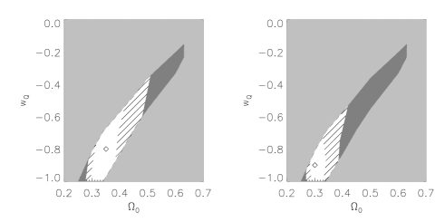
Figure 3: 90% confidence level joint constraints on $\Omega_{O}$, $w_{Q}$ from MAP 2-year data and ACT for two fiducial models (indicated by the diamond). Light gray shaded area is excluded by MAP power spectrum analysis alone, while dark gray shaded area is excluded by MAP+ACT small scale bispectrum considering only $\ell>12$. We extrapolate that the area filled with pattern can be excluded by considering also $2<\ell<12$ (see text for details). Similar constraints can be obtained from an experiment with the specifications of the Planck mission.

It is however important to bear some caveats in mind. In general $w_{Q}$ might be time dependent. The CMB power spectrum will give constraints on some “ weighted mean” of $w_{Q}(z)$. The analysis presented here constraints a different weighted mean of $w_{Q}(z)$, where most of the weight comes from $z\sim 1$. This method has to be interpreted as a first order approximation to detect $w_{Q}\neq-1$.

We have also assumed that the CMB primordial signal is gaussian and that other foregrounds contributions to the bispectrum (e.g., dust, point sources, SZ effect) can be subtracted out. While the SZ and point sources contributions can be accurately subtracted out (e.g., [10]), dust should be negligible above the galactic plane and accurate dust templates are available [25], the presence of a primordial non-gaussian signal might invalidate the results.

V Appendix

The derivation of Eq. (10) is conceptually similar to that of Spergel & Goldberg [15] for the Integrated Sachs-Wolfe effect, but is complicated by the fact that the nonlinear evolution of the power spectrum cannot be factorized in a time dependent and a scale dependent functions. We start from:

$$\langle\Theta^{*\ell_{1}}_{m_{1}}a_{\ell_{2}}^{m_{2}}\rangle=-4\left\langle\int d\hat{\gamma}_{1}d\hat{\gamma}_{2}dr\right.\frac{r_{*}-r}{r_{*}r}\Phi^{NL}(r,\hat{\gamma}_{1}r)$$

$$\times\left.\int d\tau\dot{\Phi}^{NL}(\tau,\hat{\gamma}_{2}\tau)Y^{*m_{1}}_{\ell_{1}}(\hat{\gamma}_{1})Y^{m_{2}}_{\ell_{2}}(\hat{\gamma}_{2})\right\rangle$$ (20)

where the dot denotes $\partial/\partial\tau$. Writing $\Phi$ in terms of its Fourier transform $\tilde{\Phi}$ and expanding the exponential as $\exp(k\cdot\hat{\gamma}r)=(4\pi)\sum_{\ell^{\prime}m^{\prime}}i^{\ell^{\prime}}Y^{*m^{\prime}}_{\ell^{\prime}}(\hat{\gamma}_{k})Y^{m^{\prime}}_{\ell^{\prime}}(\hat{\gamma})j_{\ell^{\prime}}(kr)$, we obtain:

$$\langle\Theta^{*\ell_{1}}_{m_{1}}a_{\ell_{2}}^{m_{2}}\rangle\!\!\! \!\!\simeq \!\!\!\!-2(4\pi)^{2}\!\!\int\!d\hat{\gamma}_{1}d\hat{\gamma}_{2}dr\frac{r_{*}-r}{r_{*}r}\!\int\!d\tau\frac{d^{3}k}{(2\pi)^{3}}i^{\ell^{\prime}+\ell^{\prime\prime}}$$ (21)

$$\!\!\!\!\!\!\times \!\!\!\!\!\dot{P}_{\Phi}(k;\tau,r)i^{\ell^{\prime}+\ell^{\prime\prime}}j_{\ell^{\prime}}(kr)Y^{*m^{\prime}}_{\ell^{\prime}}(\hat{\gamma}_{k})Y^{m^{\prime}}_{\ell^{\prime}}(\hat{\gamma}_{1})$$

$$\!\!\!\!\!\!\times \!\!\!\!\!\!Y^{*m^{\prime\prime}}_{\ell^{\prime\prime}}(\hat{\gamma}_{k})Y^{m^{\prime\prime}}_{\ell^{\prime\prime}}(\hat{\gamma}_{2})Y^{*m_{1}}_{\ell_{1}}(\hat{\gamma}_{1})Y^{m_{2}}_{\ell_{2}}(\hat{\gamma}_{2})$$

where $P_{\Phi}(k;\tau,r)$ is defined through

$$\langle\dot{\tilde{\Phi}}(k,\tau)\tilde{\Phi}(k^{\prime},r)\rangle=2(2\pi)^{3}\dot{P}_{\Phi}(k;\tau,r)\delta^{D}({\bf k}+{\bf k}^{\prime})$$ (22)

and $\delta^{D}$ denotes the Dirac delta function. In principle (21) has an extra term which vanishes at high $\ell$. Using the fact that $d^{3}k=k^{3}dkd\hat{\gamma}_{k}$ and the orthogonality relations of spherical harmonics, we obtain $\int d\hat{\gamma}_{1}d\hat{\gamma}_{2}d\hat{\gamma}_{k}$ yields $-\delta^{K}_{\ell^{\prime}\ell_{1}}\delta^{K}_{m_{1}m^{\prime}}\delta^{K}_{\ell^{\prime\prime}\ell_{2}}\delta^{K}_{m_{2}m^{\prime\prime}}\delta^{K}_{\ell^{\prime\prime}\ell^{\prime}}\delta^{K}_{m^{\prime\prime}m^{\prime}}$ , where $\delta^{K}$ denotes the Kronecker delta. Finally using the approximation:

$$\int dkk^{2}f(k)j_{\ell^{\prime}}(kr)k_{\ell^{\prime\prime}}(k\tau)\simeq f(\ell^{\prime}/r)\pi/2r^{2}\delta(r-\tau)$$ (23)

and performing the remaining integral in $d\tau$, we obtain Eq. 10.

References

(1) Jaffe, A. H. et al. 2000, Phys. Rev. Lett., 86, 3475
(2)Caldwell, R. R., Dave R., Steinhardt, P. J. 1998, Phys. Rev. Lett., 80, 1582
(3) White, M. 1998, ApJ, 506, 495
(4) Bennett, C. L. et al. 1995, BAAS, 187.7109; see also http://MAP.gsfc.nasa.gov
(5) Page L. et al. 2001, proposal submitted to NSF for the Physical Frontiers Center program.
(6) Bersanelli et al 1996, COBRAS/SAMBA Rep. Phase A study, ESA D/SCI(96)3; see also http://astro.estec.esa.nl/PLANCK/
(7) Mandolesi et al. 1998, proposal submitted to ESA for the Planck low frequency instrument
(8) Rees, M. J., Sciama D. W. 1968, Nature, 517, 611
(9) Sunyaev, R. A., Zeldovich Y. B., 1980, Ann. Rev. A. A., 18, 537
(10) Komatsu, E., Spergel, D. N. 2001, Phys.Rev. D, 63, 063002
(11) Ostriker, J. P., Vishniac E. T. 1986, ApJLett, 306, 51
(12) Sachs, R. K., Wolfe, A. M. 1967, ApJ., 147, 73
(13) Luo, X. 1994, ApJL, 427, 7
(14) Verde, L., Heavens, A. F., Matarrese, S. 2000, MNRAS, 318, 584
(15) Spergel, D. N., Goldberg, D. M. 1999, Phy. Rev. D,
59, 108001; Goldberg, D. M., Spergel D. N. 1999, Phys.Rev. D, 59, 10300
(16) Cooray, A., Hu, W. 2000, ApJ, 534, 533
(17) Zaldarriaga, M., Spergel, D.N., Seljak, U. 1987, ApJ, 488, 1
(18) Bunn, E. F., White M. 1997, ApJ, 480, 6
(19) Ma, C., Caldwell, R. R., Bode, P., Wang, L. 1999, ApJL,
521, 1
(20) Sugiyama, N. 1995, ApJS, 100, 281
(21) Peacock, J. A., Dodds, S. J. 1996, MNRAS, 267, 1020
(22) Seljak, U., Zaldarriaga, M. 1996, ApJ, 496, 337
(23) Knox, L. 1995, Phys.Rev. D, 52, 4307
(24) Christensen, N., Meyer, R., Knox, L,, Luey, B. 2001,
astro-ph/0103134; Christensen, N., Meyer, R. 2000 astro-ph/0006401
(25) Schlegel, D., Finkbeiner, D., Davis, M. 1998, ApJ, 500, 525