$UBV$ stellar photometry of bright stars in GC M5. II. Physical parameters of HB stars

Abstract

The physical parameters of the stars in the central region of the globular cluster M5 (NGC 5904) were determined from $UBV$ photometry using Kurucz (1992) (K92) synthetic flux distributions and some empirical relations. It is found that the bluest horizontal branch (HB) stars have higher luminosities than predicted by canonical zero-age horizontal branch (ZAHB) models. Parameters of the mass distribution on the HB stars are determined. It is shown that the gap in the blue HB previously reported (Markov et al. 1999, hereafter Paper I) is probably a statistical fluctuation.

1 Introduction

Crocker, Rood & O’Connel (1988, CRO88) determined spectroscopically $\log T_{\mathrm{eff}}$ and $\log g$ for $14$ BHB stars in globular cluster (GC) M5. They found that M5 BHB stars matched the canonical ZAHB models quite well. In our photometry (Paper I) there are $11$ stars common with CRO88. Assuming a relationship between the temperatures and surface gravities as derived in CRO88 and the atmospheric models of K92, we are able to obtain the physical parameters for more than $100$ BHB stars from our photometric observations.

According to Buonanno et al. (1981) (BCF81) and Crocker & Rood (1985) the bluest BHB stars tend to rise above the canonical ZAHB whilst Bohlin et al. (1985) did not find such effect. The completeness of our sample throws additional light on this matter.

The present work is structured as follows. In §2, the transformation of observed colours and magnitudes to the ($\log T_{\mathrm{eff}}$,$~{}\log L$) plane is described. In §3, an approximation of the optical colour–magnitude diagram (CMD) in terms of synthetic HBs is presented and the statistical importance of the gap in the blue HB discussed in Paper I is evaluated. §9 is dedicated on the position of BHB stars in the theoretical diagram and finally our findings are summarized in §5.

2 Physical characteristics of HB stars

We determine the effective temperatures of BHB stars from their reddening-free colours. For this purpose, we use theoretical models of energy distributions for different temperatures, gravities and abundances, in particular the line blanket atmospheres of K92. We choose the model with metallicity [Fe/H]$=-1.5$, i.e. the nearest value to that derived in Paper I ($-1.38$). It is well known that the model grids make folds on the $(U-B)_{0}$, $(B-V)_{0}$ and $(U-V)_{0}$, $(B-V)_{0}$ planes. This leads to a nonsingle-valued transformation from colours to temperatures and gravities. Unfortunately, all the BHB stars of M5 are situated just within the folds and we forfeit the opportunity for simultaneous determination of $\log T_{\mathrm{eff}}$ and $\log g$. After a suitable gravity-averaging of the atmospheric parameters, it becomes possible to achieve the necessary unequivocal dependence of the colours on the effective temperature.

The analysis of the data for BHB stars is divided into two parts. We consider separately hot BHB stars (those with $(B-V)_{0}<-0.02$) and cool BHB stars (with $(B-V)_{0}>-0.02$). The reason is that the different colour indices as temperature and gravity indicators exchange their role at about $T_{\mathrm{eff}}=9\,200\mathrm{K}$. The $(U-B)_{0}$ colours as a measure of the Balmer discontinuity and $(U-V)_{0}$ as a long baseline colours are very sensitive temperature parameters for B–type stars in the $UBV$ system. The $(B-V)_{0}$ colour is a good temperature indicator for cooler stars ($\log T_{\mathrm{eff}}<3.96$). For that reason different models are adopted to analyse the hot and cool BHB stars.

2.1 Determination of $\log T_{\mathrm{eff}}$ for hot BHB stars

The effective temperature is derived from the observed $UBV$ data using the relations $Q(\log T_{\mathrm{eff}})$ and $(U-V)_{0}(\log T_{\mathrm{eff}})$ found in K92. These relations are applied for $Q<0.0$ and $(U-V)_{0}<0.10$. Both relations are employed for $\log g$ in the interval $(3,\,4.5)$ and then the derived $T_{\mathrm{eff}}$ values are averaged. The effective temperatures for $67$ BHB stars are determined in this way. The dispersion in $\log T_{\mathrm{eff}}$ in the two cases is $\pm 0.013$ and $\pm 0.020$. The mean standard errors of $Q$ and $(U-V)_{0}$ are about $\pm 0.04$ mag, so the error in $\log T_{\mathrm{eff}}$ should not exceed $\pm 0.043$ ($\pm 1\,100$K at $T_{\mathrm{eff}}=10\,000$K).

2.2 Determination of $\log T_{\mathrm{eff}}$ for cool BHB stars

$Q$ and $(U-V)_{0}$ are no longer sensitive temperature indicators for stars in this evolutionary stage. $(B-V)_{0}$ with a maximum gravity dependence of $\Delta(B-V)_{0}=0.18$ at $\log T_{\mathrm{eff}}=3.9$ for $\log g$ in the interval $(2,\,4.5)$ is a more appropriate indicator. An assumption about $\log g$ is needed to derive the temperatures. Model computations show that $(U-B)_{0}$ is a strong gravity indicator for these stars. This is demonstrated in Fig. 7 of Paper I, where the theoretically predicted two-colour relations taken from K92 are overlaid on the observed data. As we discussed in §4 of Paper I, the majority of these HB stars show an ultraviolet deficiency and their positions are consistent with the loci of the models with ${\log g\sim 2.0}$. For this reason $\log g$ within the interval $(2,\,3.5)$ is chosen here. The model suggests a mean standard deviation for $\log T_{\mathrm{eff}}$ of $\pm 0.021$. Taking into account that the uncertainty in $(B-V)_{0}$ is about $\pm 0.04$ mag, we find the error in $\log T_{\mathrm{eff}}\sim\pm 0.045$, which corresponds to $900\mathrm{K}$ at $T_{\mathrm{eff}}{=}8\,000\mathrm{K}$.

The effective temperatures of $111$ hot and cool HB stars are obtained using this technique. A check of the validity of the determined temperatures is made by comparison with $11$ BHB stars in common between the CRO88 and our observations. Figure 1 illustrates a tendency of our temperatures to be higher on average by $0.008\pm 0.003$.

Figure 1: Comparison between the effective temperatures $\log T_{\mathrm{eff}}$ derived in this work and the CRO88 values for $11$ common stars.

Provided that the effective temperatures are determined, appropriate K92 relations ($BC\left(\log T_{\mathrm{eff}}\right)$ and $BC\left[(B-V)_{0}\right]$ for hot and cool BHB stars, respectively) are used to derive bolometric corrections (BC), and then bolometric magnitudes and luminosities. The derived luminosities are based on the assumption that $(m-M)_{V_{0}}=14.46\pm 0.03$ and $M_{\mathrm{bol}}^{\sun}=4.72$. The best fit of our observed CMD to the canonical ZAHB of Dorman et al. (1993) (DRO93) is used to obtain the distance modulus. The DRO93 evolutionary models are for [Fe/H]$=-1.48$, [O/Fe]$=0.63$, $Y_{HB}=0.25$ and core mass $M_{\mathrm{core}}=0.485$ $M_{\sun}$ (hereafter we imply only this set of DRO93 tracks when we refer to the evolutionary theory). The mean square error of the luminosity determinations is $\pm 0.1$ in $\log L$. The ($\log L$, $\log T_{\mathrm{eff}}$) diagram for all $111$ BHB stars with $UBV$ magnitudes in our sample is given in Fig. 2.

Figure 2: $\left(\log L,\,\log T_{\mathrm{eff}}\right)$ diagram for all $111$ BHB stars (solid circles) with $UBV$ magnitudes in our sample. The open  triangles denote $14$ stars of CRO88. The solid line is the ZAHB of Dorman et al. (1993).

The stars of CRO88 with spectroscopically measured atmospheric characteristics are also plotted as open triangles.

2.3 Determination of the stellar masses

Knowing the effective temperatures, luminosities and surface gravities of the stars, we can estimate the corresponding masses independently of their evolutionary history through the relation $M/L\sim g/T_{\mathrm{eff}}^{4}$ or in more convenient form

$$\log\left(M/M_{\sun}\right)=\log\left(L/L_{\sun}\right)-4\log T_{\mathrm{eff}}+\log g+10.611.$$

We rely on a sample of $12$ BHB stars with reliable $\log g$ and $\log T_{\mathrm{eff}}$ data (CRO88) to derive a linear relation between surface gravity and effective temperature. A least square fit yields:

$$\log g=-11.244(\pm 1.929)+3.699(\pm 0.478)\,\log T_{\mathrm{eff}}\,.$$ (1)

Equation (1) is deduced for stars with $\log T_{\mathrm{eff}}$ in the interval $(3.948,\,4.145)$, and it is used to obtain the surface gravities of all BHB stars with r.m.s. $\sim 0.15$, which corresponds to the errors in the input data.

The errors of the mass determination consist of both the errors of $\log T_{\mathrm{eff}}$ and $\log g$, and those of $\log L$. Assuming errors in $\log T_{\mathrm{eff}}$ of $\pm 0.043$, in $\log g$ of $\pm 0.15$, and in $\log L$ of $\pm 0.1$ we obtain a mean error in the mass derivation of approximately $\pm 0.19$. Changes in the adopted distance modulus and extinction would result in a systematic shift of the derived masses. The dependence of the stellar mass on the effective temperature is shown in Fig. 3. The distribution of the masses of $62$ stars situated within the temperature range ($8\,800\,$K, $14\,000\,$K) of validity of the linear relation $\log g\left(\log T_{\mathrm{eff}}\right)$ is plotted in an inset on Fig. 3.

Figure 3: (mass,$\,\log T_{\mathrm{eff}}$) diagram. The solid circles are stars with obtained masses. The $12$ stars of CRO88 are plotted as open triangles. The solid line is the (ZA mass,$~{}\log T_{\mathrm{eff}}$) relation; the dotted line is the relation between the stellar mass and maximal temperature reachable during the post-ZAHB evolution; the dashed line is the isochrone at $t=110\,\mathrm{Myr}$. The inset shows the mass distribution.

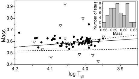
During their HB lifetime, the stars reach a maximal effective temperature (see, for instance, DRO93). This temperature as a function of stellar mass is also represented in Fig. 3 by dotted line. It almost completely coincides with the isochrone at  $t=60\,$Myr. Although the error of the stellar masses is considerable, Figure 3 implies that the masses of the hottest stars ($\log T_{\mathrm{eff}}>4.07$) are systematically higher than those corresponding to the limit temperatures. This suggests a discrepancy in luminosity compared with theory. The masses of the $12$ stars of CRO88 are also plotted in Figure 3 (open triangles). The big scatter of these stars around the zero-age relation can be interpreted as an inaccurate determination of the surface gravities (see Table 2 of CRO88).

3 HB synthetic ($M_{V}$, $(U-V)_{0}$) diagram

3.1 Parameterisation of the HB

A curve (ridge line), which is close enough to a HB strip, is determined by means of averaging the stellar positions on small segments covering the HB. A position along the HB, from the red extreme toward the blue end, is given by arc length ($\ell_{\mathrm{HB}}$) of the normal projection on the ridge line (for similar procedures, see Rood and Crocker 1989; Ferraro et al. 1992; Dixon et al. 1996).

The ridge line and HB region of M5 is shown in Fig. 4 (dashed line).

Figure 4: Colour–magnitude diagram of the HB region of the M5 and the ridge line (dashed line) used to build the stellar distribution along the HB. Solid line is the ZAHB of DRO93.

To make possible a comparison of our distribution to other ones, we give the scale ratios $\Delta\ell_{\mathrm{HB}}/\Delta(U-V)_{0}=3.341$ and $\Delta\ell_{\mathrm{HB}}/\Delta M_{V}=2.468$. The values of the HB red extreme of the ridge line are $M_{V}^{\mathrm{RE}}=0.43$ and  $(U-V)_{0}^{\mathrm{RE}}=0.7$, the blue and red edges of the instability strip at the level of the ridge line are $(U-V)_{0}^{\mathrm{IS}_{\mathrm{B}}}=0.26$ and  $(U-V)_{0}^{\mathrm{IS}_{\mathrm{R}}}=0.45$ (see Fig. 4). The observed distribution is shown in Fig. 5 both as a histogram and a cumulative frequency.

Figure 5: The observed stellar distribution along the HB in M5. The histogram of the $\ell_{\mathrm{HB}}$–coordinate of the stars is represented on panel (a) and the cumulative frequency – on panel (b).

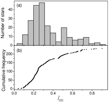
The $\ell_{\mathrm{HB}}$–values of the blue and red edges of the instability strip are $\ell_{\mathrm{HB}}^{\mathrm{IS}_{\mathrm{B}}}=0.244$ and $\ell_{\mathrm{HB}}^{\mathrm{IS}_{\mathrm{R}}}=0.143$.

3.2 Theoretical models of the HB

To create a model HB, we transform the mass-age relation (after ZAHB) into a colour-magnitude plane using the theoretical correspondence between the (mass, age) and ($\log L$,$~{}\log T_{\mathrm{eff}}$) or ($\log g$,$~{}\log T_{\mathrm{eff}}$) relations. Evolutionary tracks (DRO93), synthetic atmospheres (K92), the adopted metallicity, and distance modulus are the same as in §2. A Hermite interpolation (Kahaner et al. 1988) of the DRO93 tracks is employed. We adopt both a unimodal (Gaussian) mass distribution and a bimodal one (see e.g. Rood 1973; Lee et al. 1990; Dixon et al. 1996).

An assembly of $76$ RRLyrae stars randomly distributed in the instability strip in ($M_{V}$, $(B-V)_{0}$) plane with a mean magnitude $\langle V_{\mathrm{RR}}\rangle=15.09$ (Reid 1996) is added. From the CMD, the blue edge of the instability strip is located at $(B-V)_{0}^{\mathrm{IS}_{\mathrm{B}}}=0.16$ and the red edge – at $(B-V)_{0}^{\mathrm{IS}_{\mathrm{R}}}=0.38$ (for comparison see BCF81). The adopted number of variable stars is derived under condition that the sample represents $74$ per cent of all HB stars located in the measured region.

Taking into account the weak dependence of the HB lifetime on the total mass of the stars, we can introduce a universal HB lifetime $\sim 110$ Myr. Due to the assumption of a constant rate of populating the ZAHB, the ages after the ZAHB are considered as random numbers uniformly distributed in the range $0$–$110$ Myr. We also presume known stellar mass distribution as well as age distribution. For a unimodal mass distribution (UMD) the transformation method (Box–Muller algorithm) is used to produce the Gaussian deviates, whereas in the case of a bimodal mass distribution (BMD) the appropriate deviates are generated by means of the rejection method. Normally distributed random ‘observational’ errors are introduced at the end of the mapping.

To restrict the unknown parameters of the mass distribution that produce the observed CMD, we compare statistically the corresponding distributions of synthetic and observed HBs. A two-sample Kolmogorov–Smirnov (KS) test is used to check the null hypothesis that model and observed cumulative $\ell_{\mathrm{HB}}$–frequencies ($\ell_{\mathrm{HB}}$–curves) are drawn from the same parent distribution. Simultaneously a chi-square ($\chi^{2}$) test is applied to binned $\ell_{\mathrm{HB}}$–coordinate distributions. Each synthetic HB contains the same number of stars as our observed sample. At the $99$ per cent level of significance, we disprove the null hypothesis for all parameters outside the regions listed in Table 1.

Model	Parameter	Permissible interval	Best fit
UMD	$\left\langle M_{\mathrm{HB}}\right\rangle$	$\left(0.5801,0.6782\right)M_{\sun}$	$0.6327M_{\sun}$
	$\sigma_{M_{\mathrm{HB}}}$	$\left(0.0179,0.0433\right)M_{\sun}$	$0.0321M_{\sun}$
BMD	$\left\langle M_{\mathrm{HB}}\right\rangle_{1}$	$\left(0.5699,0.6432\right)M_{\sun}$	$0.6057M_{\sun}$
	$\sigma_{\left(M_{\mathrm{HB}}\right),1}$	$\left(0.0181,0.0199\right)M_{\sun}$	$0.0192M_{\sun}$
	$\left\langle M_{\mathrm{HB}}\right\rangle_{2}$	$\left(0.6110,0.6850\right)M_{\sun}$	$0.6493M_{\sun}$
	$\sigma_{\left(M_{\mathrm{HB}}\right),2}$	$\left(0.0258,0.0288\right)M_{\sun}$	$0.0274M_{\sun}$
	$f_{1}$	$\left(0.3703,0.4054\right)$	$0.3898$

Table 1: Permissible intervals of the parameters determining the model mass distributions and their best-fitting values.

$\left\langle M_{\mathrm{HB}}\right\rangle$ and $\sigma_{M_{\mathrm{HB}}}$ are the mean value and the standard deviation of the Gaussian mass distributions, respectively. In the case of bimodal mass distribution, we have an additional parameter $f_{1}$, the fraction of HB stars contributed by the first Gaussian. The mean values of the significant levels $\left\langle Q_{\mathrm{KS}}\right\rangle$ and $\left\langle Q_{\chi^{2}}\right\rangle$ are obtained by generating $\sim 250\,000$ synthetic HBs with the best-fitting parameters (see Table 1). When the UMD is used $\left\langle Q_{\mathrm{KS}}\right\rangle=0.43$ and $\left\langle Q_{\chi^{2}}\right\rangle=0.17$, whereas in the case of BMD $\left\langle Q_{\mathrm{KS}}\right\rangle=0.48$ and $\left\langle Q_{\chi^{2}}\right\rangle=0.25$, which makes the second distribution preferable.

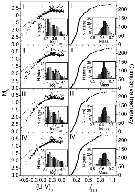
Figure 6 shows four synthetic HBs computed by means of UMD, as well as the corresponding cumulative distributions of coordinates, the histograms of masses and temperatures.

Figure 6: Four synthetic HBs randomly chosen from the set of  $\sim 250\,000$  HB simulations and cumulative frequency of $\ell_{\mathrm{HB}}$–coordinate, which are computed by unimodal mass distribution. The insets show the histograms of the $T_{\mathrm{eff}}$ and mass distributions. The dashed line is the ridge line.

Similar results are plotted on Figure 7 for bimodal mass distribution.

Figure 7: Same as in Figure 6, but for the bimodal mass distribution.

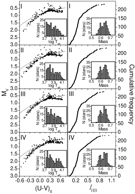
In both cases (UMD and BMD) the corresponding four synthetic HBs are chosen randomly from the whole sets of   HB simulations. At first glance, there are considerable differences between the separate synthetic HBs although the model assumptions are just the same. The principal cause is that the random deviates used for the mass generation only asymptotically approach the desired distributions. However, a thorough inspection reveals that the blue tails of UMD synthetic HBs are less populated and more extended than tails of the BMD synthetic HBs – a prospective effect due to the bigger distribution tail area of the unimodal mass distribution.

The main discrepancy between the observed and model HBs is the downward deviation of the synthetic blue tails from the ridge line. Both UMD and BMD computations show the same tendency. The formal cause may be the inconsistency of the uniform distribution of the stellar ages after ZAHB adopted in the computations, although, most probably, the real cause is the unreliability of canonical evolution theory.

3.3 Gaps on the blue HB

Even a passing glance at the simulated HBs ascertains substantial statistical fluctuations, which modify their morphology. The observed gap discussed in Paper I may thus be such a fluctuation. We consider as gaps regions with a local minimum of the slope of a monotonically increasing cumulative frequency function. The standard procedure to test the statistical significance of suspected gaps is based on the assumption that the probability to find stars along the cumulative distribution is uniform with a value $P_{L}$ left of the gap, and uniform with another value $P_{R}$ right of the gap (Aisenman et al. 1969). Usually, the significance of this hypothesis is not taken into account. Instead, one verifies whether the probability of finding stars in the gap substantially differs from the mean of the probabilities $P_{L}$ and $P_{R}$ (Howarden 1971). When applied to cumulative $\ell_{\mathrm{HB}}$-distributions of HB stars, the standard method yields a local highly overestimated statistical significance of the gaps. In the present work, we apply KS-test to a section of $\ell_{\mathrm{HB}}$-curve in length of five gap widths in order to examine the hypothesis of uniform distribution around and in the gap (probably with three different densities).

The observed gap should be represented as a domain on the ($W$, $\ell_{\mathrm{HB}}$) plane ($W$ is the gap width) because of photometric errors. To derive the borders of this region, we vary the stellar magnitudes and colours within photometric accuracy bounds reported in Paper I, and produce a set of $\sim 200\,000$ modified observed HBs. Then, we obtain the joint probability density function (PDF) of the observed gap $f_{o}\left(W,\ell_{\mathrm{HB}}\right)$ using an automatic search and inspection of arising intervals. Three elliptic-like contours (with major axes in ordinate direction) containing $95$, $50$, and $5$ per cent of all detected gaps are plotted on Figure 8 to depict this function.

Figure 8: Characteristics of the observed and detected gaps on the synthetic HBs computed for UMD and BMD.

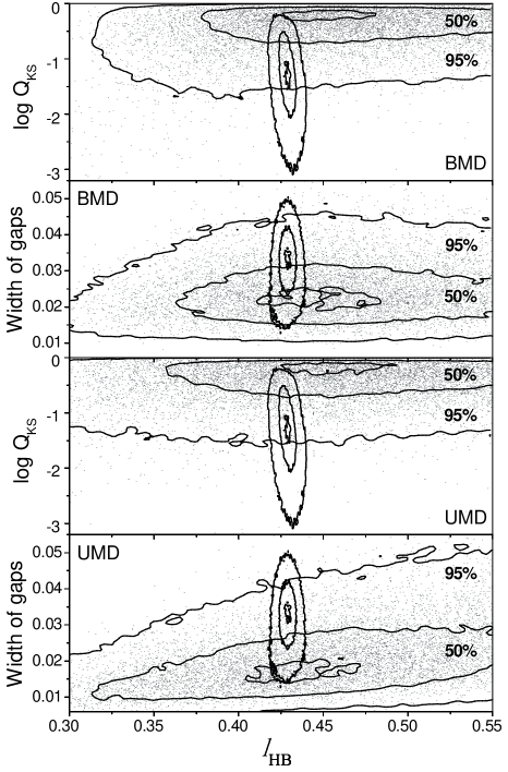
As mentioned in §7, the difference between the models and observed data is statistically non-significant. This enables us to use the estimation of a mere chance probability that a gap comparable with the observed one may appear on the synthetic HBs. We consider the width and the location of the biggest gap on the simulated $\ell_{\mathrm{HB}}$-curves as random variables. The significant level $Q_{KS}$ of the gap region can also be interpreted as a random parameter, which is a function of the gap sharpness. We construct the sampling distributions empirically by using the set of $\sim 250\,000$ simulated HBs. The joint PDFs $f_{s}\left(W,\ell_{\mathrm{HB}}\right)$ and $f_{s}\left(Q_{KS},\ell_{\mathrm{HB}}\right)$ are depicted on Figure 8 as isodensity contours containing $95$, $50$, and $5$ per cent of all revealed gaps. The gaps are also plotted as points.

To test the null hypothesis that there is no genuine difference (within the limits of random variability) between the parameters of observed and model gaps, we use the following three probabilities (see Appendix A). $P_{1}$ and $P_{2}$ are the averaged (over $f_{o}$) probabilities of arising of synthetic gaps, which are wider than the observed one. They are calculated by the marginal PDF ($m_{s}(W)$ for the ($W$, $\ell_{\mathrm{HB}}$) relation and $m_{s}(Q_{KS})$ for the ($Q_{KS}$, $\ell_{\mathrm{HB}}$) relation) and by a conditional PDF ($f_{s}(W|\ell_{\mathrm{HB}})$ and $f_{s}(Q_{KS}|\ell_{\mathrm{HB}})$), correspondingly. $P_{2}$ takes account of location on the $\ell_{\mathrm{HB}}$-curve as distinct from $P_{1}$. $P_{3}$ is the probability of appearance of synthetic gaps outside the region enclosed in the averaged (over $f_{o}$) isodensity curve on which the observed gap is situated. The so-defined probabilities for the ($W$, $\ell_{\mathrm{HB}}$) and ($Q_{KS}$, $\ell_{\mathrm{HB}}$) relations are given in Table 2.

	UMD model			BMD model
Relation	$P_{1}$	$P_{2}$	$P_{3}$	$P_{1}$	$P_{2}$	$P_{3}$
($W$, $\ell_{HB}$)	0.21	0.10	0.30	0.20	0.20	0.48
(log $Q_{KS}$, $\ell_{HB}$)	0.08	0.08	0.16	0.09	0.08	0.17

Table 2: Probabilities used to test statistical significance of the observed gap.

By the conventional standard of statistical significance (probability $<0.05$), the observed gap is non-significant. Therefore, the observed gap is not so extraordinary, as it seems to be, and we tend to consider it as a statistical fluctuation.

4 BHB stars and the theoretical H–R diagram

In the ($\log L,~{}\log T_{\mathrm{eff}}$) plane (Fig. 2), the tendency for the blue end of the HB to rise above the ZAHB (the oxygen-enhanced models (DRO93) for [Fe/H]$=-1.48$) is obvious. BCF81 and Crocker & Rood (1985) have found the same effect, using different methods and models for transforming the observational data from a ($V$,$~{}\left(B-V\right)$) plane into the theoretical ($\log L$,$~{}\log T_{\mathrm{eff}}$) plane. On the other hand, Bohlin et al. (1985) have not confirmed this trend (their Figure 7) when perform ultraviolet observations with a rocket-borne telescope near $1540$Å  and  $2360$Å  for $50$ BHB stars.

An important argument for the validity of an upward trend is the location in the ($\log L$,$~{}\log T_{\mathrm{eff}}$) diagram of those $14$ BHB stars with atmospheric parameters being already measured spectroscopically (CRO88). They are plotted in Fig. 2 as open triangles. On canonical theory we expect the observed HB to be close to the ZAHB (DRO93). One possibility for the revealed disagreement is that we have underestimations of the adopted photometric errors. To check this we use $11$ stars in common with CRO88. From the K92 temperature–colours calibrations we compute the corresponding $(U-V)_{0}$, $(U-B)_{0}$ and $(B-V)_{0}$ values for each star. The mean differences between the model and the observed colours are as follows: $\Delta(U-V)_{0}=0.02$,  $\Delta(U-B)_{0}=0.01$, and $\Delta(B-V)_{0}=0.02$ – values comparable within $1\sigma$ of our photometric errors.

It can be seen from Fig. 9, where the theoretical ZAHB is fitted to our observed data, that the blue end of the observed HB (dots) do not match the model of DRO93 (solid line).

Figure 9: ($M_{V}$,$~{}(B-V)_{0}$) diagram (panel (a)) and ($M_{V}$,$~{}\log T_{\mathrm{eff}}$) diagram (panel (b)) for BHB stars with $UBV$ photometry. Open triangles denote the stars of CRO88. Solid line is the ZAHB (DRO93). Dashed line on the panel (a) is the fiducial line of Sandquist et al. (1996).

This discrepancy has already been noted by Sandquist et al. (1996). The fiducial line of BHB derived by these authors is plotted for comparison as dashed line in Fig. 9a. Sandquist et al. (1996) assume that the disagreement results from the colour calibration. However, the fact, that the high temperature stars with spectroscopically obtained temperatures also have much higher luminosities (see Fig. 2) than the predicted ones, means that the observed effect cannot be explained by the colour calibration only. In Fig. 9b, we compare the positions of these stars (open triangles) (the $V$ mag for three of them are taken from BCF81) with the location of the model HB. It is evident that stars with $\log T_{\mathrm{eff}}>4.04$ deviate upward from the model with $\Delta M_{V}$ in the range ($-0.2$ to $-0.5$). These values are too large to be explained with photometric errors. A similar effect of ‘over–luminosity’, reaching $\sim 0.4$ mag has been found by Grundahl et al. (1998) in the globular cluster M13 using Stromgren photometry. Moreover, according to Grundahl et al. (1999) all stars with $T_{\mathrm{eff}}>11\,500\,$K in $14$ GCs demonstrate a systematical deviation from the canonical ZAHB in the sense of being brighter or hotter than the models. This effect is independent of the metallicity, the mixing history on the RGB, and other cluster parameters. The results in Fig. 2 are in a remarkable agreement with their results.

In explanation of this effect, we note that apart from the most popular picture, in which HB stars are distributed along ZAHB because of differences in the amount of mass loss during the ‘He–flash’ at the RGB tip, Fusi Pecci & Renzini (1978) focused attention on the possible effect of stellar rotation. With a suitable choice of parameters the blue end of the ‘rotational’ ZAHB is expected to be more luminous than the non-rotating canonical one.

The standard method used in §2 to obtain physical parameters of the BHB stars does not permit simultaneous determination of the effective temperature and the surface gravity. The latter parameter is lost during the inevitable averaging inherent to the elimination of the ambiguity of the Kurucz grids (see §2). For that reason we cannot confirm independently the effect found in $6$ GCs including M5 (Moehler et al., 1995; Moehler, 1999), which consists in a displacement from the ZAHB to lower $\log g$ of the bluest HB stars having spectroscopically measured surface gravities. We shall only remark that the linear relation (1) shows the same tendency to ‘under–gravity’ towards the bluest HB stars in M5. Grundahl et al. (1999) reveal the same connection between the ‘over–luminosity’ and the ‘under–gravity’ in $14$ GCs, and suppose that these effects are different manifestations of a uniform physical mechanism. Relying on the spectroscopic data for field and GC BHB stars, the authors (Grundahl et al. 1999) hypothesize that this physical mechanism consists in radiative levitation of elements heavier than carbon and nitrogen into the stellar atmosphere, rather than a stellar interior or evolution effects.

Formally, the possibility for a displacement toward higher luminosities of some stars due to evolution off the ZAHB cannot be ignored. Moreover, when the BHB stars reach the HB lifetime they demonstrate the ‘under–gravity’ effect simultaneously with the ‘over–luminosity’. However, according to the canonical evolutionary theory (DRO93) and the adopted concept of constant evolution rate onto the ZAHB, there is no well-grounded reason that so many low mass stars being at the same time in a transient evolutionary phase as core helium exhaustion.

5 Summary

In the present paper we have applied standard methods to determine the stellar physical parameters using a new $UBV$ stellar photometry for the HB stars of the GC M5. Comparing the observed $UBV$ colours with K92 synthetic atmospheres, we have derived the effective temperatures and luminosities of a large sample of BHB stars. The surface gravities have been derived assuming a linear relation between spectroscopically measured $\log g$ and $T_{\mathrm{eff}}$ of $12$ stars (CRO88).

We have found considerably high luminosities for the bluest HB stars than predicted by the canonical theory.

Approximations of the distribution of stars in the ($M_{V}$,$~{}(U-V)_{0}$) diagram have been performed under assumptions of unimodal and bimodal mass distributions.

The statistical importance of the observed gap in the blue HB at $\ell_{\mathrm{HB}}=0.42$ has been studied by simulations. We conclude that it is a statistical fluctuation.

Appendix A Definitions of the probabilities used to test statistical significance of the observed gap

For the sake of completeness, we present definitions of the probabilities $P_{1}$, $P_{2}$, and $P_{3}$ used in §2. We restrict our attention only to the $\left(W,\ell_{\mathrm{HB}}\right)$ relation.

$$P_{1}=\int\left(1-\int\limits_{0}^{W}m_{s}\left(\overline{W}\right)d\overline{W}\right)\,m_{o}\left(W\right)\,\,dW\,,$$

$$P_{2}=\int\int\frac{\left(1-\int\limits_{0}^{W}f_{s}\left(\overline{W},\ell_{\mathrm{HB}}\right)d\overline{W}\right)}{m_{s}\left(\ell_{\mathrm{HB}}\right)}f_{o}\left(W,\ell_{\mathrm{HB}}\right)\,\,dW\,d\ell_{\mathrm{HB}}\,,$$

where $f_{o}\left(W,\ell_{\mathrm{HB}}\right)$ and $f_{s}\left(W,\ell_{\mathrm{HB}}\right)$ are joint PDFs of the observed and synthetic gaps, $m_{s}\left(W\right)$, $m_{s}\left(\ell_{\mathrm{HB}}\right)$ and $m_{o}\left(W\right)$ are the marginal PDFs of the $f_{s}\left(W,\ell_{\mathrm{HB}}\right)$ and $f_{o}\left(W,\ell_{\mathrm{HB}}\right)$. The integration is performed over domain in $\left(W,\ell_{\mathrm{HB}}\right)$ plane with $f_{o}\left(W,\ell_{\mathrm{HB}}\right)>0$.

$$P_{3}=\int\int\,f_{s}\left(W,\ell_{\mathrm{HB}}\right)\,dW\,d\ell_{\mathrm{HB}}$$

with a region of integration determined by the inequality

$$f_{s}\left(W,\ell_{\mathrm{HB}}\right)<\int\int\,f_{s}\left(W,\ell_{\mathrm{HB}}\right)f_{o}\left(W,\ell_{\mathrm{HB}}\right)\,\,dW\,d\ell_{\mathrm{HB}}\,.$$

References

- [1] Aisenman, M. L., Demarque, P., Miller, R. H. 1969, ApJ, 155, 973
- [2] Bohlin, R. C., Cornett, R. H., Hill, J. K., Smith, A. M. & Stecher, T. P. 1985, ApJ , 292, 687
- [3] Buonanno, R., Corsi, C. E., & Fusi Pecci F. 1981, MNRAS, 196, 435 (BCF81)
- [4] Crocker D.A., Rood R.T., 1985, in ‘Horizontal-Branch and UV-Bright Stars’, ed. by A. G. Davis Philip (L. Davis Press), 107
- [5] Crocker, D. A., Rood, R. T., & O’Connel, O. W. 1988, ApJ, 332, 236 (CRO88)
- [6] Dorman, B., Rood, R. T., & O’Connell, R. W. 1993, ApJ, 419, 596 (DRO93)
- [7] Dixon, W. V., Davidsen, A. F., Dorman, B., & Ferguson, H. C. 996, AJ, 111, 1936
- [8] Grundahl, F., Vandenberg Don A., & Andersen, M. I. 1998, ApJ, 500, L179
- [9] Grundahl, F., Catelan, M., Landsman, W. B., Stetson, P. B. & Andersen, M. I. 1999, ApJ, submitted
- [10] Ferraro, F. R., Fusi Pecci, F., & Buonanno, R. 1992, MNRAS, 256, 376
- [11] Fusi Pecci, F., Renzini A., 1978, in IAU Symp. 80, The HR Diagram, ed. by A.G.D.Philip, D.S.Hayes (Reidel:Dordrecht), 225
- [12] Hawarden, T. G. 1971, Observatory, 91, 78
- [13] Kahaner, D., Moler, C., & Nash, S. 1988, Numerical Methods and Software (Prentice Hill)
- [14] Kurucz, R. L. 1992, in IAU Symp. 149, The Stellar Populations of Galaxies, ed. by B.Barbuy and A.Renzini (Dordreht:Kluwer), 225 (K92)
- [15] Lee, Y.-W., Demarque, P., & Zinn, R 1990, ApJ, 350, 155
- [16] Markov, H. S., Spassova, N. M. & Baev, P. V. 1999, MNRAS, submitted (Paper I)
- [17] Moehler, S., Heber, U. & Boer, K. S. 1995, A&A, 294, 65
- [18] Moehler, S 1999, Reviews in Modern Astronomy, 12
- [19] Reid, N. 1996, MNRAS 278, 367
- [20] Rood, R. T. 1973, ApJ, 184, 815
- [21] Rood, R. T. & Crocker, D. A. 1989 in IAU Colloquium 111, The Use of Pulsating Stars in Fundamental Problems of Astronomy, ed. by F. G. Schmidt (Cambridge University Press:Cambridge), 103
- [22] Sandquist, E. L., Bolte, M., Stetson, P. B., & Hesser, J. R. 1996, ApJ, 470, 910