The Shape of Spectral Breaks in GRB Afterglows

Abstract

Gamma-Ray Burst (GRB) afterglows are well described by synchrotron emission from relativistic blast waves expanding into an external medium. The blast wave is believed to amplify the magnetic field and accelerate the electrons into a power law distribution of energies promptly behind the shock. These electrons then cool both adiabatically and by emitting synchrotron and inverse Compton radiation. The resulting spectra is known to consist several power law segments, which smoothly join at certain break frequencies. Here, we give a complete description of all possible spectra under those assumptions, and find that there are 5 possible regimes, depending on the ordering of the break frequencies. The flux density is calculated by integrating over the contributions from all the shocked region, using the Blandford McKee solution. This allows us to calculate more accurate expressions for the value of these break frequencies, and describe the shape of the spectral breaks around them. This also provides the shape of breaks in the light curves caused by the passage of a break frequency through the observed band. These new, more exact, estimates are different from more simple calculations by up to a factor of $\sim 70$, and describe some new regimes which where previously ignored.

1. Introduction

In recent years, several dozens of gamma-ray burst (GRB) afterglows have been observed, and data is accumulating rapidly. The quality of these observations is constantly improving. The study of afterglow emission has helped shed light on many important aspects of the GRB phenomenon. The spectrum during the afterglow phase is well described by synchrotron emission from a relativistic blast wave, and consists of several power law segments (PLSs), that join at several break frequencies (e.g. Sari, Piran & Narayan 1998). These break frequencies are the self absorption frequency, $\nu_{a}$, below which the optical depth to synchrotron self absorption is larger than unity, $\nu_{m}$, the typical synchrotron frequency of the minimal electron in the power-law, and $\nu_{c}$, the synchrotron frequency of an electron whose cooling time equals the dynamical time of the system. Granot, Piran & Sari (2000) have then found that if $\nu_{c}<\nu_{m}$, the self absorption frequency actually splits into two: $\nu_{ac}$ and $\nu_{sa}$, where an optical depth of unity is produced by non-cooled electrons and all electrons respectively. Different possible orderings of these break frequencies result in five possible spectral regimes, as shown in figure 1.

The physical parameters of a burst may be deduced from fitting the observed broad band spectrum to the theoretical spectrum. This has been done by Wijers & Galama (1999) for GRB 970508 by fitting a broken power law theoretical spectrum. A detailed description of the shape of the spectrum allowed a more accurate determination of the self absorption frequency $\nu_{sa}$ and the peak frequency $\nu_{m}$ (Granot, Piran & Sari 1999b, hereafter GPS99b). A more accurate theoretical calculation of the break frequencies leads to a more accurate conversion from the observed spectrum to the burst parameters. The combined effect was that the inferred value of the density, for example, was different than that of Wijers and Galama by two orders of magnitude. This illustrates the sensitivity of this method to the shape of the theoretical spectrum around the break points, and stresses the need for a more accurate determination of the theoretical break frequencies, for all various spectral breaks.

So far only the shape of the spectrum around $\nu_{m}$ (Granot, Piran & Sari 1999a, hereafter GPS99a; Gruzinov & Waxman 1999) and $\nu_{a}$ (GPS99b) was calculate in detail, and even that was only done for the canonical case where $\nu_{sa}<\nu_{m}<\nu_{c}$ (see the upper panel of figure 1). This paper, is intended to extend these works for all spectral breaks, and therefore provide a comprehensive, self consistent calculation of the broad band spectrum. We provide analytic formulas which approximate the shape of each of the spectral breaks and their positions, in a form which is easy to use for afterglow fitting. We also suggest a prescription for combining these breaks to a single analytic broad band spectrum.

The physical model is outlined in §2, while a more detailed and formal description of the model and of the calculation of the observed flux density is given in §6 (Appendix A). Our main results are presented in §3. In §4 we give prescriptions for combining the shapes of the spectrum near the different spectral breaks into a single analytic broad band spectrum. We discuss our results in §5.

2. The Physical Model

An exact calculation of the spectrum requires the knowledge of (i) The hydrodynamic quantities (bulk Lorentz factor and number density) (ii) The magnetic field strength (iii) The electron energy distribution. These should be given for any location behind the shock, and at any time. Below we describe our approach to all three.

(i) The hydrodynamics is described by the Blandford McKee (1976, BM hereafter) self similar solution. This solution describes a spherical relativistic blast wave expanding into a cold medium, and assumes an adiabatic flow, i.e. that radiation losses are small and do not effect the hydrodynamics. Radiative effects can be taken into account to modify the hydrodynamic evolution as described by (Sari 1997, Cohen, Piran & Sari 1998) and to modify the structure of the cooling layer behind the shock as described by Granot & Königl (2001). If the radiative losses are not too large, our formalism would give the correct break frequencies and break shapes, provided that one uses the time dependent energy, as discussed in the first two of these references. The BM solution we use is for an impulsive explosion in an ambient density described by a power law with radius, $\rho_{\rm ext}(r)=Ar^{-k}$. We consider two different values of $k$ which are of particular physical interest: $k=0$, corresponding to an interstellar medium (ISM), and $k=2$, corresponding to a massive star progenitor, surrounded by its pre-explosion wind. The assumption of a spherical flow is also adequate for a jetted flow at sufficiently early times, when the Lorentz factor of the flow is still larger than the inverse opening angle of the jet. We therefore have the complete hydrodynamic description in term of the total energy $E$, and the external number density $n_{\rm ext}$ (or $A$ in the case of wind). The hydrodynamic profile that is used, is given in equations 14 through 16.

(ii) We assume the magnetic field gets a fixed fraction, $\epsilon_{B}$, of the internal energy everywhere behind the shock, as given by equation 12. This would be the case if the shock amplified, randomly oriented, magnetic field decreases due to adiabatic expansion. Different assumptions on the evolution and orientation of the magnetic field were shown to have only a small effect on the resulting spectrum (GPS99a,b).

(iii) The electrons are assumed to acquire a power law distribution of energies, $N(\gamma)\propto\gamma^{-p}$ for $\gamma\geq\gamma_{{\rm min},0}$, immediately behind the shock. Their total energy immediately behind the shock is a fraction $\epsilon_{e}$ of the internal energy. After being accelerated by the shock, the electrons cool due to radiative losses and adiabatic cooling. The former can be calculated from synchrotron theory and the latter from the density profile given in by the BM solution. The resulting distribution is given in equation 23.

Given the above, the observed flux density may be calculated as described in §6 (Appendix A). The spectrum for the optically thin breaks may be calculated using equation 24, while equation 34 applies more generally.

3. Results

power law segments. All five possible different spectra, which are shown in Figure 1, consist of between three and five different power law segments (PLSs). At each asymptotic PLS (sufficiently far from the break frequencies) we have $F_{\nu}\propto\nu^{\beta}t^{\alpha}$. Altogether there are eight different PLSs, labeled A through H, from high to low values of $\beta$. Note that there are two different PLSs with a slope of $\beta=1/3$. Both are produced by the low energy tail of synchrotron radiation, but in region $D$ it is the non-cooled electrons that are responsible for the radiation while in region $E$ it is the cooled electrons. Most PLSs appear in more than one of the five possible spectra (see Figure 1). If one is only interested in the spectrum far enough from the break frequencies, then the normalizations of the different PLSs is all that is needed to accurately describe the spectrum. This is given in Table 1. The coefficients for PLSs A, G and H, slightly depend on $p$ in a non analytic way. These were calculated for $p=2.2,2.5,3$, and a linear function (or a linear function multiplied by an exponent) was used to describe the results.

For PLS E, we find that the emission becomes dominated by the contribution from small radii (i.e. early times when the radius of the shock was small) for $k\geq 23/13\approx 1.769$. The electrons responsible for the emission in this regime have suffered considerable adiabatic cooling (as well as radiative losses). In this regime ($k>23/13$) PLS E splits into two different PLSs, whose spectral slope $\beta$ depends on $k$. Furthermore, the effective size of the afterglow image, at a given observed time, in this regime depends on the observed frequency. However, since this new regime is somewhat out of the main stream of this paper, and in order to avoid confusion, we leave the detailed description of this new regime to a future work (Granot & Sari, in preparation). The normalization of PLS E, and the expressions for the spectral breaks $b=10,11$ (that involve PLS E), are therefor left out of Tables 1 and 2, respectively, for $k=2$.

break frequencies. The different possible combinations of the eight PLSs, result in 11 different break frequencies, labeled $b=1,...,11$ (see Figure 1). Again, the same break frequency may appear in more than one spectrum. The values of the break frequencies, $\nu_{b}$, and the corresponding extrapolated flux densities, $F_{\nu_{b},{\rm ext}}$, are defined at the point where the asymptotic PLSs meet. These can be directly calculated from the normalization of the PLSs that are given in Table 1, but for completeness they are given explicitly in Table 2. The fit for the $p$ dependence was redone in this table (with either a linear fit, an exponent or a combination of the two) using the accurate results for $p=2.2,2.5,3$, therefore resulting in slight (a few percent) inconsistencies with the previous table.

shape of breaks. The Flux density near a spectral break, $\nu_{b}$, may be approximated by

$$F_{\nu}=F_{\nu_{b},{\rm ext}}\times\left[\left({\nu/\nu_{b}}\right)^{-s\beta_{1}}+\left({\nu/\nu_{b}}\right)^{-s\beta_{2}}\right]^{-1/s}\ ,$$ (1)

where $\beta_{1}$ and $\beta_{2}$ are the asymptotic spectral slopes below and above the break, respectively, and $s$ is a parameter which describes the sharpness of each break. The sign of $s$ is equal to that of $\beta_{1}-\beta_{2}$ (i.e. positive if the spectral slope decreases across the break), while $|s|$ represents the sharpness of the break (the sharper the break, the larger $|s|$). The shape of most spectral breaks (except for $b=1,8,10,11$), depends on the value of $p$, and so does the corresponding value of $s=s(p)$, which is given in Table 2. All quantities which depend on the value of $p$ were calculated for $p=2.2,2.5,3$, and are given in a form which is as exact as the functional parameterization permits at these values of $p$, and interpolates (or extrapolates) for other values of $p$, and should therefore be reasonably accurate for $1.5\lesssim p\lesssim 3.5$ (see discussion below equation 11 for $p<2$).

The break $b=1$ has been investigated in detail by GPS99a, for $k=0$, and they found that the physically motivated formula

$$F_{\nu}=F_{\nu_{1},{\rm ext}}\left[1-\exp(-\tau_{1})\right]\tau_{1}^{-6/5}\quad,\quad\tau_{1}=(\nu/\nu_{1})^{-5/3}\ ,$$ (2)

provides an even better description of $F_{\nu}$ near the break (with an MRD of $2.63\%$, compared to $6.78\%$ with equation 1). However, for $k=2$, equation 1 provides a better fit (with an MRD of $1.02\%$ compared to $25\%$ with equation 2), which shows that the previous success of equation 2 was accidental.

Equations 1 and 2 both give a poor fit for $b=4$. This is because the spectral slope across this break does not change monotonically. We therefore provide an alternative formula for this break,

$$F_{\nu}=F_{\nu_{4},{\rm ext}}\left[\phi_{4}^{2}\exp(-s\phi_{4}^{2/3})+\phi_{4}^{5/2}\right]\quad,\quad\phi_{4}=\nu/\nu_{4}\quad\ ,$$ (3)

where the values of $s$ for $b=4$ which appear in Table 2, are for this equation, rather than for equation 1, as for the other breaks.

4. A Prescription For The Broad Band Spectra

The values and the shape of the break frequencies, as given in the previous section, are strictly valid only when the break frequencies are far away from each other. Though, in principle, our formalism is adequate to describe the general spectrum, for arbitrary values of the break frequencies, such a description, would require a new calculation for any ratio of the break frequencies, and is therefore not practical. Instead, we choose to give a heuristic prescription, that uses the shapes from the previous section to construct a broad band spectrum, which includes all the breaks, for an arbitrary ratio of the break frequencies. Once again we stress that this is not a rigorous derivation of such a spectrum, but simply an analytic equation, that gives a smooth spectrum when the break frequencies are close to each other, and approaches the rigorous shape of each break, in the asymptotic situation where the break frequencies are far apart. Such an equation is useful for fitting afterglow data.

One can readily construct such a formula for any one of the five different possible spectra shown in Figure 1. Let us label these spectra 1 through 5, from top to bottom, and denote the corresponding flux densities by $F_{\nu}^{(i)}$ where $i=1,...,5$. We also label the flux density near the 11 spectral breaks by $F_{b}$, where $b=1,...,11$. The fluxes, $F_{b}$, are given by equation 1 (for break $b=4$ equation 3 gives a more accurate description). Now, let us define a quantity $\tilde{F}_{b}$, by

$$\tilde{F}_{b}=\left[1+\left({\nu/\nu_{b}}\right)^{s(\beta_{1}-\beta_{2})}\right]^{-1/s}\ .$$ (4)

The formulas for the rounded shape of the spectrum for the five spectra which are shown in Figure 1, from top to bottom, are given by

$$F_{\nu}^{(1)} = F_{1}\tilde{F}_{2}\tilde{F}_{3}\ ,$$ (5)

$$F_{\nu}^{(2)} = F_{4}\tilde{F}_{5}\tilde{F}_{3}\ ,$$ (6)

$$F_{\nu}^{(3)} = F_{4}\tilde{F}_{6}\ ,$$ (7)

$$F_{\nu}^{(4)} = F_{7}\tilde{F}_{8}\tilde{F}_{9}\ ,$$ (8)

$$F_{\nu}^{(5)} = F_{7}\tilde{F}_{10}\tilde{F}_{11}\tilde{F}_{9}\ .$$ (9)

The first term, $F_{b}$, provides the normalization and the shape of the spectrum near the lowest break frequency, while each consecutive term, $\tilde{F}_{b}$, represents the next break frequency, from low to high frequencies, and provides the shape of the spectrum near that break frequency, and the appropriate change in the spectral slope across the break. The number of free parameters in each spectrum generally equals the number of break frequencies plus two, since besides the values of the break frequencies, one has to specify the value of $p$ and of the flux normalization. The bottom panel of figure 1 is an exception, and $F_{\nu}^{(5)}$ has only 5 free parameters, since there is a closure relation between the four break frequencies (Granot, Piran & Sari 2000):

$${\nu_{10}\over\nu_{7}}\left({\nu_{11}\over\nu_{9}}\right)^{4/5}=h(p)\sim 1\quad({\rm for}\ k=0)\ .$$ (10)

Our prescription for constructing the broad band spectrum uses $F_{\nu_{b},{\rm ext}}$ from only one of the break frequencies in each spectrum, and thus avoids the problem of the slight inconsistencies within Table 2 (that arise due to the independent fits for the $p$ dependence, e.g. §3).

5. Discussion

We have used the BM solution, to obtain more accurate expressions for the flux density. Under the assumptions that the initial electron distribution is a strict power-law with a low energy cutoff, and that the magnetic field is amplified immediately behind the shock, we derived exact expressions for the values of the break frequencies, as well as the shape of the spectrum around each break. We have given a complete general description of the broad band spectrum. As our analysis is general, it also includes exotic spectra, that may only be relevant in very early phases or for extreme parameters. Our main results are summarized in Figure 1 and Tables 1 and 2.

In general, the spectrum of GRB afterglows evolves from fast to slow cooling. For example, for an ISM with standard parameters, (e.g. $n_{0}\cong 1$,$E_{52}\cong 1$, $\epsilon_{B}\cong 0.01$) the initial spectrum is 5, then $\nu_{m}$ crosses $\nu_{c}$ and the spectrum turns into spectrum 1, and finally, when $\nu_{m}$ crosses $\nu_{sa}$ the spectrum turns into spectrum 2. The transition times between the various spectra of Figure 1 can be worked out by equating the various frequencies, as given in Table 3. It follows that there are two types of evolution depending on the parameters, as given in the chart below.

$${\rm ISM}=\cases{5\rightarrow 1\rightarrow 2&$n_{0}E_{52}^{4/7}\epsilon_{B}^{9/7}<18$\cr 4\rightarrow 3\rightarrow 2&$n_{0}E_{52}^{4/7}\epsilon_{B}^{9/7}>18$}$$

$${\rm WIND}=\cases{4\rightarrow 5\rightarrow 1\rightarrow 2&$A_{*}\bar{\epsilon}_{e}\,^{-1}E_{52}^{-3/7}\epsilon_{B}^{2/7}>100$\cr 4\rightarrow 3\rightarrow 2&$A_{*}\bar{\epsilon}_{e}\,^{-1}E_{52}^{-3/7}\epsilon_{B}^{2/7}$ < 100}$$

The weakest link in our formalism, is the assumption of a sharp lower cutoff in the electron distribution. This would affect breaks $b=1,2,4,7,9$ (though for $b=1$, the shape of the break will not be effected, while $\nu_{1}$ and $F_{\nu_{1},{\rm ext}}$ may change). Nevertheless, our calculation provides the first self consistent description of all these breaks. The values and shape of the rest of the breaks, depends only on the assumption of a power-law distribution, well above the low energy cutoff, and on the electron cooling. Our description of these breaks ($b=3,5,6,8,10,11$) is therefore more robust. These breaks may still be somewhat affected by the assumption of the magnetic field evolution. However, in previous papers (GPS99a,b), we have shown that this dependence is relatively week ($F_{\nu_{2},{\rm ext}}$ and $\nu_{2}$ change by up to $\sim 50\%$, while $F_{\nu_{1},{\rm ext}}$ and $\nu_{1}$ change only by up to a few percent, where in both cases the shape of the break does not change considerably).

We give a complete description of all possible power-law segments (PLSs), and provide exact expressions for the flux density away from the break frequencies. These expression are useful when partial information for the afterglow exists. In general a spectral slope and a flux at some frequency are sufficient to give some constraint on the afterglow parameters (in PLSs G and H, $p$ would also be needed). For example, if only X-ray data exists, PLS H can be used to extract some information on the underlying parameters, and if only radio data exists, PLS B can be used, even if the self absorption frequency is not observed, (i.e. is above the observed radio frequency).

Expressions for some of the break frequencies and corresponding flux densities already exist in the literature (Waxman 1997; Sari, Piran & Narayan 1998; Wijers & Galama 1999; GPS99a,b; Granot, Piran & Sari 2000; Chevalier & Li 2000; Panaitescu & Kumar 2000). Most of these works address the spectrum shown in the upper panel of Figure 1 (spectrum 1). The values we obtain for the break frequencies and corresponding flux densities are in some cases significantly different than previous estimates (by up to a factor of $\sim 70$). For $k=0$ and $p=2.5$, our value for $\nu_{2}$ ($F_{\nu_{2},{\rm ext}}$), which is better known as $\nu_{m}$ ($F_{\nu_{m}}$), is a factor of 1.3 (4.2) larger (smaller) than Sari, Piran & Narayan (1998), a factor of 1.5 (3.1) smaller (larger) than Wijers & Galama (1999), a factor of 3.8 (for $\nu_{2}$) smaller than Panaitescu & Kumar, and a factor of 15 (8) smaller (larger) than Waxman (1997). For $p=2.2$ our value for $\nu_{2}$ is a factor of 70 smaller than Waxman (1997). Our values for $\nu_{2}$ and $F_{\nu_{2},{\rm ext}}$ are only slightly different (by $-5.1\%$ and $+1.6\%$, respectively) than GPS99a, due to a small approximation they made for the local emissivity. Our value for $\nu_{3}$ ($\nu_{c}$) is a factor of 2.6 larger than Sari, Piran & Narayan (1998), a factor of 6.4 larger than Wijers & Galama (1999), and a factor of 6.1 larger than Panaitescu & Kumar. Our value for $\nu_{1}$ ($\nu_{sa}$) is a factor of 1.9 larger than Waxman (1997), a factor of 3.7 smaller than Wijers & Galama (1999), a factor of 4.1 larger than Panaitescu & Kumar, and a factor of 2.1 smaller than GPS99b. For $k=2$ (and $p=2.5$), our values of $\nu_{1}$, $\nu_{2}$ and $\nu_{3}$ are smaller by factors of 2.5, 1.4 and 1.4, respectively, compared to Chevalier & Li (2000), while our value for $F_{\nu_{2},{\rm ext}}$ is larger by a factor of 3.2; Compared to Panaitescu & Kumar, or value for $\nu_{1}$ ($\nu_{2}$) is larger (smaller) by a factor of 4.9 (7.4), while our value for $\nu_{3}$ is larger by only $16\%$. Our expressions for the break frequencies and corresponding flux densities of spectra 4 and 5 (bottom two panels of Figure 1), for $k=0,2$, are different by up to a factor of $3$ from those given in Granot, Piran & Sari (2000).

Our equations do not include the effects of inverse compton scattering on the cooling of the electrons. This effect is known to be important, when $\epsilon_{B}\ll\epsilon_{e}$ (Sari, Narayan & Piran 1996, Panaitescu & Kumar 2000, Sari & Esin 2001). Following the prescription of Sari & Esin, we can include the effects of inverse compton by inserting appropriate powers of $(1+Y)$ into the values of the break frequencies, or the PLSs (where $Y$ is the compton y-parameter). PLSs C, E, F and H should be multiplied by $(1+Y)^{-3/8}$, $(1+Y)^{2/3}$, $(1+Y)^{-1}$ and $(1+Y)^{-1}$, respectively.

Preliminary results from this work have already been used successfully in fitting the data of several afterglows (e.g. Galama et al. 2000; Harrison et al. 2001). In the latter case the first evidence for inverse Compton emission was found. A special effort has been made to present the results of our model in a way that is simple to implement, and would provide the most accurate results to date for spherical afterglows, or jetted afterglows within their quasi spherical phase (before any significant lateral spreading).

6. Appendix A

The energy density $e$, number density $n$, magnetic field $B$, and random Lorentz factor of the electrons $\gamma_{e}$, are measured in the local rest frame of the fluid, in addition to all the primed quantities. The remaining quantities are measured in the lab frame, i.e. the rest frame of the ambient medium in which the flow is spherical. We use a spherical coordinate system in this rest frame, where the z-axis points at the observer. The time, $t$, measured in this rest frame is called the coordinate time, and is to be distinguished from the time, $t^{\prime}$, measured in the local rest frame of the fluid, and from the observer (or observed) time, $t_{\rm obs}$, at which the emitted photons reach the observer. The subscript ‘$0$’ denotes the value of a quantity just behind the shock.

The initial electron distribution, just behind the shock, is given by

$$N(\gamma_{e})=K_{0}\gamma_{e}^{-p}\ \ {\rm for}\ \ \gamma_{e}\geq\gamma_{{\rm min},0}={\bar{\epsilon}_{e}e_{0}\over n_{0}m_{e}c^{2}}\ ,$$ (11)

where $m_{e}$ is the electron rest mass and $K_{0}=(p-1)n_{0}\gamma_{{\rm min},0}^{p-1}$. Note, that the above equation is usually written using $\epsilon_{e}=\bar{\epsilon}_{e}(p-1)/(p-2)$, which is the fraction of the internal energy given to the electrons. The advantage of using $\bar{\epsilon}_{e}$, is that it makes most equations somewhat simpler. Furthermore, it will apply also for the case $p<2$, as long as the minimal Lorentz factor is proportional to the shock Lorentz factor. The magnetic field is assumed to hold a constant fraction, $\epsilon_{B}$, of the internal energy, everywhere,

$$B^{2}=8\pi\epsilon_{B}e\ .$$ (12)

The evolution of the Lorentz factor of each electron is described by

$${d\gamma_{e}\over dt^{\prime}}=-{\sigma_{T}B^{2}\over 6\pi m_{e}c}\gamma_{e}^{2}+{\gamma_{e}\over 3n}{dn\over dt^{\prime}}\ .$$ (13)

The first term on the right hand side of equation 13 represents the radiative losses while the second term represents adiabatic cooling. The radiative term includes only synchrotron losses. A simple prescription of how to include the effects of enhanced electron cooling, due to inverse compton scattering, on the observed synchrotron emission, is given in §5.

We use the BM spherical self-similar solution for an impulsive explosion, where the external medium is cold and its density changes as a power law of the distance from the center, $\rho_{\rm ext}(r)=Ar^{-k}$, $k<4$ (extensions for $k>4$ are given in Best and Sari 2000, but were not used in this paper). The derivations are made for a general value of $k<4$, and are then used for $k=0$ and $k=2$, which are of special physical interest. According to this solution, the proper energy density, Lorentz factor and proper number density of the shocked fluid are given by

$$e = 2\Gamma^{2}\rho_{\rm ext}c^{2}\chi^{-(17-4k)/3(4-k)}\ ,$$ (14)

$$\gamma = 2^{-1/2}\Gamma\,\chi^{-1/2}\ ,$$ (15)

$$n = 2^{3/2}\Gamma n_{\rm ext}\,\chi^{-(10-3k)/2(4-k)}\ ,$$ (16)

where $\Gamma$ is the Lorentz factor of the shock, and

$$\chi=\left[1+2(4-k)\Gamma^{2}\right]\left(1-{r\over ct}\right)\ .$$ (17)

The $\chi$ coordinate of a fluid element is given by

$$\chi=\left({R\over R_{0}}\right)^{4-k}=\left({t\over t_{0}}\right)^{4-k}$$ (18)

where $R_{0}$ and $t_{0}$ are the shock radius and coordinate time, respectively, when the fluid element crosses the shock. Since $\Gamma^{2}\propto t^{k-3}$, we obtain that

$${\gamma\over\gamma_{0}}=\chi^{-{(7-2k)\over 2(4-k)}}\quad,\quad{n\over n_{0}}=\chi^{-{(13-2k)\over 2(4-k)}}\quad,\quad{e\over e_{0}}=\left({B\over B_{0}}\right)^{2}=\chi^{-{2(13-2k)\over 3(4-k)}}\ .$$ (19)

Using equation 19 and the relation $dt^{\prime}=dt/\gamma$, we can write equation 13 in terms of $\chi$:

$${d\gamma_{e}\over d\chi}=\,-\,{\sigma_{T}B_{0}^{2}t_{0}\chi^{-(49-8k)/6(4-k)}\gamma_{e}^{2}\over 6(4-k)\pi m_{e}c\gamma_{0}}\,-\,{(13-2k)\over 6(4-k)}{\gamma_{e}\over\chi}\ .$$ (20)

Solving equation 20 we obtain

$$\gamma_{e}(\gamma_{e,0},\chi)={\gamma_{e,0}\over\chi^{(13-2k)/6(4-k)}+\gamma_{e,0}/\gamma_{\rm max}(\chi)}\ ,$$ (21)

where $\gamma_{e,0}\equiv\gamma_{e}(\chi=1)$ is the initial Lorentz factor of the electron, just behind the shock, and $\gamma_{\rm max}(\chi)$ is the maximal Lorentz factor at $\chi>1$, which corresponds to an electron with $\gamma_{e,0}\to\infty$, and is given by

$$\gamma_{\rm max}(\chi)={2(19-2k)\pi m_{e}c\gamma_{0}\over\sigma_{T}B_{0}^{2}t_{0}}\left({\chi^{(25-2k)/6(4-k)}\over\chi^{(19-2k)/3(4-k)}-1}\right)\ .$$ (22)

The fraction of electrons with a Lorentz factor within the interval $[\gamma_{e},\gamma_{e}+d\gamma_{e}]$ is given by: $N(\gamma_{e})d\gamma_{e}/n$, and remains constant as all these quantities evolve with increasing $\chi$. The electron distribution is therefore given by:

$$N(\gamma_{e},\chi)=$$ (23)

$$K_{0}\chi^{(2k-13)(p+2)\over 6(4-k)}\gamma_{e}^{-p}\left(1-{\gamma_{e}\over\gamma_{\rm max}(\chi)}\right)^{p-2}\ \ {\rm for}\ \ \ \gamma_{\rm min}(\chi)\leq\gamma_{e}\leq\gamma_{\rm max}(\chi)$$

where $\gamma_{\rm min}(\chi)=\gamma_{e}(\gamma_{{\rm min},0},\chi)$.

We now have explicit expressions for both the hydrodynamical quantities and the electron distribution, over all relevant space-time, and can calculate the flux density near the various break frequencies. For breaks that are in the optically thin regime (b=2,3,9,11) one may use the equation

$$F_{\nu}(t_{\rm obs})={2(4-k)R_{l}^{3}(1+z)\over d_{L}^{2}}\int^{1}_{0}dy\int^{y^{k-4}}_{1}d\chi{\chi y^{2(5-k)}P^{\prime}_{\nu^{\prime}}(y,\chi,t_{\rm obs})\over\left[1+(7-2k)\chi y^{4-k}\right]^{2}}\ .$$ (24)

which is a generalization of equation 13 of GPS99a, where $d_{L}$ and $z$ are the luminosity distance and cosmological redshift of the source, respectively, $P^{\prime}_{\nu^{\prime}}$ is the radiated power per unit volume per unit frequency in the local rest frame of the fluid, and should be taken at the coordinate time $t=t_{z}+r\mu/c$, where $t_{z}\equiv t_{\rm obs}/(1+z)$,

$$R_{l}=\left[{(17-4k)(4-k)Et_{z}\over 4\pi Ac}\right]^{1/(4-k)}\ ,$$ (25)

$$\gamma_{l}=\left[{(17-4k)E\over 4^{5-k}(4-k)^{3-k}\pi Ac^{5-k}t_{z}^{3-k}}\right]^{1/2(4-k)}\ ,$$

$E$ is the energy of the blast wave, $y\equiv R/R_{l}$ (e.g. GPS99a),

$$\mu\equiv\cos(\theta)\cong 1-{1-\chi y^{4-k}\over 4(4-k)\gamma_{l}^{2}y}\ ,$$ (26)

and $\nu^{\prime}=\nu\gamma(1-\beta\mu)$. The Spectral emissivity of a single electron (in the fluid rest frame) is given by

$$P^{\prime}_{\nu^{\prime},e}={\sqrt{3}q_{e}^{3}B\sin\alpha\over m_{e}c^{2}}\,F\left({\nu^{\prime}\over\nu^{\prime}_{\rm syn}}\right)\quad,\quad\nu^{\prime}_{\rm syn}={3q_{e}B\gamma_{e}^{2}\sin\alpha\over 4\pi m_{e}c}\ ,$$ (27)

where $q_{e}$ is the electric charge of the electron, $\alpha$ is the pitch angle between the direction of the electron’s velocity and the magnetic field, in the local rest frame of the fluid, and $F$ is the standard synchrotron function (e.g. Rybicki & Lightman 1979). In order to obtain an expression for $P^{\prime}_{\nu^{\prime}}$ (which appears in equation 24) we average $P^{\prime}_{\nu^{\prime},e}$ over $\alpha$, assuming an isotropic distribution of electrons in the local rest frame,

$$P^{\prime}_{\nu^{\prime},e,{\rm iso}}=\int_{0}^{\pi/2}d\alpha\sin\alpha\,P^{\prime}_{\nu^{\prime},e}(\sin\alpha)\ ,$$ (28)

and then integrate over the electron distribution,

$$P^{\prime}_{\nu^{\prime}}=\int_{\gamma_{\rm min}}^{\gamma_{\rm max}}d\gamma_{e}N(\gamma_{e})P^{\prime}_{\nu^{\prime},e,{\rm iso}}(\gamma_{e})\ .$$ (29)

For the remaining spectral breaks (b=1,4,5,6,7,8,10), where the system is not always optically thin, we follow the formalism of GPS99b. Since the emission is isotropic in the local rest frame of the fluid, the emission coefficient is simply $j^{\prime}_{\nu^{\prime}}=P^{\prime}_{\nu^{\prime}}/4\pi$, where $P^{\prime}_{\nu^{\prime}}$ is given by equation 29. The absorption coefficient is given by

$$\alpha^{\prime}_{\nu^{\prime}}={1\over 8\pi m_{e}\nu^{\prime 2}}\int_{\gamma_{\rm min}}^{\gamma_{\rm max}}d\gamma_{e}{N(\gamma_{e})\over\gamma_{e}^{2}}{\partial\over\partial\gamma_{e}}\left[\gamma_{e}^{2}P^{\prime}_{\nu^{\prime},e,{\rm iso}}(\gamma_{e})\right]\ .$$ (30)

Since the flow is spherically symmetric, the afterglow image is circular, with physical radius of

$$R_{\perp,{\rm max}}={(5-k)^{k-5\over 2(4-k)}\over\sqrt{2}}{R_{l}\over\gamma_{l}}=$$ (31)

$$\left[{2^{2-k}(17-4k)(4-k)^{5-k}Ec^{3-k}t_{z}^{5-k}\over\pi(5-k)^{5-k}A}\right]^{1/2(4-k)}\ ,$$

and for a given observer time, $t_{\rm obs}$, the specific intensity (or brightness), $I_{\nu}$, depends only on the normalized radius from the center of the image,

$$x\equiv{R_{\perp}\over R_{\perp,{\rm max}}}=(4-k)^{-1/2}(5-k)^{5-k\over 2(4-k)}\sqrt{y-\chi y^{5-k}}\ ,$$ (32)

where $x=0$ at the center of the image and $x=1$ at the outer edge of the image. As discussed in GPS99b, $I_{\nu}(x)$ may be obtained by solving the radiative transfer equation,

$${dI_{\nu}\over ds}=j_{\nu}-\alpha_{\nu}I_{\nu}\ ,$$ (33)

where $s$ is the distance along the trajectory of a photon to the observer, and the flux density is given by

$$F_{\nu}(t_{\rm obs})=2\pi(1+z)\left[{R_{\perp,{\rm max}}(t_{\rm obs})\over d_{L}}\right]^{2}\int_{0}^{1}x\,dx\,I_{\nu}(x,t_{\rm obs})\ .$$ (34)

We note that $I_{\nu}(x)$ provides the surface brightness profile of the afterglow image, that is necessary for detailed calculations of microlensing or scintillation. The surface brightness profiles that were calculated according to this formalism, have already been used to study the microlensing of GRB afterglows (Granot & Loeb 2001; Gaudi, Granot & Loeb 2001), and are presented therein.

When a break frequency is sufficiently far from other break frequencies, the spectrum near this break frequency assumes a self similar form. These self similar forms of the spectrum near the different break frequencies are presented in §3.

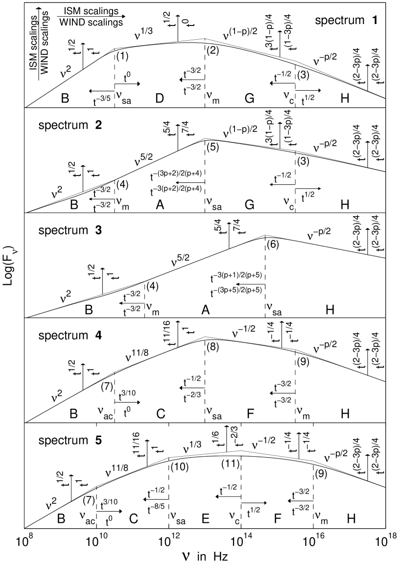
Figure 1.— The different possible broad band synchrotron spectra from a relativistic blast wave, that accelerates the electrons to a power law distribution of energies. The thin solid line shows the asymptotic power law segments (PLSs), and their points of intersection, where the break frequencies, $\nu_{b}$, and the corresponding flux densities, $F_{\nu_{b},{\rm ext}}$, are defined. The different PLSs are labeled A through H, while the different break frequencies are labeled 1 through 11. The temporal scalings of the PLSs and the break frequencies, for an ISM ($k=0$) or stellar wind ($k=2$) environment, are indicated by the arrows. The thick solid line shows the spectrum we calculated in this paper, where the broad band spectrum is constructed according to the prescription suggested in §4. The different spectra are labeled 1 through 5, from top to bottom. The relevant spectrum is determined by the ordering of the break frequencies. The top two panels (spectra 1 and 2) correspond to slow cooling ($\nu_{m}<\nu_{c}$). Spectrum 1 applies when $\nu_{sa}<\nu_{m}$, while spectrum 2 applies when $\nu_{m}<\nu_{sa}<\nu_{c}$. The two bottom panels (spectra 4 and 5) correspond to fast cooling ($\nu_{c}<\nu_{m}$). Spectrum 5 applies when $\nu_{sa}<\nu_{c}$, and spectrum 4 applies when $\nu_{c}<\nu_{sa}<\nu_{m}$. Spectrum 3 (middle panel) applies when $\nu_{sa}>\nu_{m},\nu_{c}$, where in this case the relative ordering of $\nu_{c}$ and $\nu_{m}$ is unimportant (i.e. spectrum 3 may apply both to slow cooling or fast cooling).

Table 1The Normalization of the Different Power Law Segments

PLS	$\beta$	$F_{\nu}(k=0)$ in mJy	$F_{\nu}(k=2)$ in mJy
A	$5/2$	$1.18(4.59-p)10^{8}(1+z)^{9/4}\epsilon_{B}^{-1/4}n_{0}^{-1/2}E_{52}^{1/4}t_{\rm days}^{5/4}d_{L28}^{-2}\nu_{14}^{5/2}$	$2.96(4.59-p)10^{7}(1+z)^{7/4}\epsilon_{B}^{-1/4}A_{*}^{-1}E_{52}^{3/4}t_{\rm days}^{7/4}d_{L28}^{-2}\nu_{14}^{5/2}$
B	$2$	$4.20{(3p+2)\over(3p-1)}10^{9}(1+z)^{5/2}\bar{\epsilon}_{e}n_{0}^{-1/2}E_{52}^{1/2}t_{\rm days}^{1/2}d_{L28}^{-2}\nu_{14}^{2}$	$1.33{(3p+2)\over(3p-1)}10^{9}(1+z)^{2}\bar{\epsilon}_{e}A_{*}^{-1}E_{52}t_{\rm days}d_{L28}^{-2}\nu_{14}^{2}$
C	$11/8$	$8.01\cdot 10^{5}(1+z)^{27/16}\epsilon_{B}^{-1/4}n_{0}^{-5/16}E_{52}^{7/16}t_{\rm days}^{11/16}d_{L28}^{-2}\nu_{14}^{11/8}$	$3.28\cdot 10^{5}(1+z)^{11/8}\epsilon_{B}^{-1/4}A_{*}^{-5/8}E_{52}^{3/4}t_{\rm days}d_{L28}^{-2}\nu_{14}^{11/8}$
D	$1/3$	$27.9{(p-1)\over(3p-1)}(1+z)^{5/6}\bar{\epsilon}_{e}^{-2/3}\epsilon_{B}^{1/3}n_{0}^{1/2}E_{52}^{5/6}t_{\rm days}^{1/2}d_{L28}^{-2}\nu_{14}^{1/3}$	$211{(p-1)\over(3p-1)}(1+z)^{4/3}\bar{\epsilon}_{e}^{-2/3}\epsilon_{B}^{1/3}A_{*}E_{52}^{1/3}d_{L28}^{-2}\nu_{14}^{1/3}$
E	$1/3$	$73.0(1+z)^{7/6}\epsilon_{B}n_{0}^{5/6}E_{52}^{7/6}t_{\rm days}^{1/6}d_{L28}^{-2}\nu_{14}^{1/3}$	$\cdots$
F	$-1/2$	$6.87(1+z)^{3/4}\epsilon_{B}^{-1/4}E_{52}^{3/4}t_{\rm days}^{-1/4}d_{L28}^{-2}\nu_{14}^{-1/2}$	$6.68(1+z)^{3/4}\epsilon_{B}^{-1/4}E_{52}^{3/4}t_{\rm days}^{-1/4}d_{L28}^{-2}\nu_{14}^{-1/2}$
G	$(1-p)/2$	$0.461(p-0.04)e^{2.53p}(1+z)^{3+p\over 4}\bar{\epsilon}_{e}^{p-1}\epsilon_{B}^{1+p\over 4}n_{0}^{1/2}E_{52}^{3+p\over 4}t_{\rm days}^{3(1-p)\over 4}d_{L28}^{-2}\nu_{14}^{1-p\over 2}$	$3.82(p-0.18)e^{2.54p}(1+z)^{5+p\over 4}\bar{\epsilon}_{e}^{p-1}\epsilon_{B}^{1+p\over 4}A_{*}E_{52}^{1+p\over 4}t_{\rm days}^{1-3p\over 4}d_{L28}^{-2}\nu_{14}^{1-p\over 2}$
H	$-p/2$	$0.855(p-0.98)e^{1.95p}(1+z)^{2+p\over 4}\bar{\epsilon}_{e}^{p-1}\epsilon_{B}^{p-2\over 4}E_{52}^{2+p\over 4}t_{\rm days}^{2-3p\over 4}d_{L28}^{-2}\nu_{14}^{-p/2}$	$0.0381(7.11-p)e^{2.76p}(1+z)^{2+p\over 4}\bar{\epsilon}_{e}^{p-1}\epsilon_{B}^{p-2\over 4}E_{52}^{2+p\over 4}t_{\rm days}^{2-3p\over 4}d_{L28}^{-2}\nu_{14}^{-p/2}$

Note. — The first two columns give the labels and the spectral slope, $\beta$, of the different PLSs (see Figure 1), while the last two columns give the asymptotic flux density within each PLS, for $k=0$ and $k=2$. The reader is reminded that $\bar{\epsilon}_{e}=\epsilon_{e}(p-2)/(p-1)$ depends on $p$. The notation $Q_{x}$ stands for the quantity $Q$ in units of $10^{x}$ times the (c.g.s) units of $Q$, while $t_{\rm days}$ is the observed time in days, and $A_{*}$ is $A$ in units of $5\cdot 10^{11}\,{\rm gr/cm}$ (Chevalier & Li 2000).

Table 2The Break Frequencies and Corresponding Flux Densities

$b$	$\beta_{1}$	$\beta_{2}$	$\nu_{b}$	$\nu_{b}(p)$ in Hz	$F_{\nu_{b},{\rm ext}}(p)$ in mJy	$s(p)$	MRD in %
				$1.24{(p-1)^{3/5}\over(3p+2)^{3/5}}10^{9}(1+z)^{-1}\bar{\epsilon}_{e}^{\;-1}\epsilon_{B}^{1/5}n_{0}^{3/5}E_{52}^{1/5}$	$0.647{(p-1)^{6/5}\over(3p-1)(3p+2)^{1/5}}(1+z)^{1/2}\bar{\epsilon}_{e}^{\;-1}\epsilon_{B}^{2/5}n_{0}^{7/10}E_{52}^{9/10}t_{\rm days}^{1/2}d_{L28}^{-2}$	1.64	6.68
1	2	${1\over 3}$	$\nu_{sa}$	$8.31{(p-1)^{3/5}\over(3p+2)^{3/5}}10^{9}(1+z)^{-2/5}\bar{\epsilon}_{e}^{\;-1}\epsilon_{B}^{1/5}A_{*}^{6/5}E_{52}^{-2/5}t_{\rm days}^{-3/5}$	$9.19{(p-1)^{6/5}\over(3p-1)(3p+2)^{1/5}}(1+z)^{6/5}\bar{\epsilon}_{e}^{\;-1}\epsilon_{B}^{2/5}A_{*}^{7/5}E_{52}^{1/5}t_{\rm days}^{-1/5}d_{L28}^{-2}$	1.06	1.02
				$3.73(p-0.67)10^{15}(1+z)^{1/2}E_{52}^{1/2}\bar{\epsilon}_{e}^{2}\epsilon_{B}^{1/2}t_{\rm days}^{-3/2}$	$9.93(p+0.14)(1+z)\epsilon_{B}^{1/2}n_{0}^{1/2}E_{52}d_{L28}^{-2}$	1.84-0.40p	5.9
2	${1\over 3}$	${1-p\over 2}$	$\nu_{m}$	$4.02(p-0.69)10^{15}(1+z)^{1/2}E_{52}^{1/2}\bar{\epsilon}_{e}^{2}\epsilon_{B}^{1/2}t_{\rm days}^{-3/2}$	$76.9(p+0.12)(1+z)^{3/2}\epsilon_{B}^{1/2}A_{*}E_{52}^{1/2}t_{\rm days}^{-1/2}d_{L28}^{-2}$	1.76-0.38p	7.2
				$6.37(p-0.46)10^{13}e^{-1.16p}(1+z)^{-1/2}\epsilon_{B}^{-3/2}n_{0}^{-1}E_{52}^{-1/2}t_{\rm days}^{-1/2}$	$4.68\,e^{4.82(p-2.5)}10^{3}(1+z)^{p+1\over 2}\bar{\epsilon}_{e}^{p-1}\epsilon_{B}^{p-{1\over 2}}n_{0}^{p\over 2}E_{52}^{p+1\over 2}t_{\rm days}^{1-p\over 2}d_{L28}^{-2}$	1.15-0.06p	1.9
3	${1-p\over 2}$	$-{p\over 2}$	$\nu_{c}$	$4.40(3.45-p)10^{10}e^{0.45p}(1+z)^{-3/2}\epsilon_{B}^{-3/2}A_{*}^{-2}E_{52}^{1/2}t_{\rm days}^{1/2}$	$8.02\,e^{7.02(p-2.5)}10^{5}(1+z)^{p+{1\over 2}}\bar{\epsilon}_{e}^{p-1}\epsilon_{B}^{p-{1\over 2}}A_{*}^{p}E_{52}^{1/2}t_{\rm days}^{{1\over 2}-p}d_{L28}^{-2}$	0.80-0.03p	4.4
				$5.04(p-1.22)10^{16}(1+z)^{1/2}\bar{\epsilon}_{e}^{2}\epsilon_{B}^{1/2}E_{52}^{1/2}t_{\rm days}^{-3/2}$	$3.72(p-1.79)10^{15}(1+z)^{7/2}\bar{\epsilon}_{e}^{5}\epsilon_{B}n_{0}^{-1/2}E_{52}^{3/2}t_{\rm days}^{-5/2}d_{L28}^{-2}$	$3.44p-1.41$	0.7
4	2	${5\over 2}$	$\nu_{m}$	$8.08(p-1.22)10^{16}(1+z)^{1/2}\bar{\epsilon}_{e}^{2}\epsilon_{B}^{1/2}E_{52}^{1/2}t_{\rm days}^{-3/2}$	$3.04(p-1.79)10^{15}(1+z)^{3}\bar{\epsilon}_{e}^{5}\epsilon_{B}A_{*}^{-1}E_{52}^{2}t_{\rm days}^{-2}d_{L28}^{-2}$	$3.63p-1.60$	1.8
				$3.59(4.03-p)10^{9}e^{2.34p}\left[{\bar{\epsilon}_{e}^{4(p-1)}\epsilon_{B}^{p+2}n_{0}^{4}E_{52}^{p+2}\over(1+z)^{6-p}t_{\rm days}^{3p+2}}\right]^{1/2(p+4)}$	$20.8(p-1.53)e^{2.56p}d_{L28}^{-2}\left[{(1+z)^{7p+3}\epsilon_{B}^{2p+3}E_{52}^{3p+7}\over\bar{\epsilon}_{e}^{10(1-p)}t_{\rm days}^{5(p-1)}}\right]^{1/2(p+4)}$	1.47-0.21p	5.9
5	${5\over 2}$	${1-p\over 2}$	$\nu_{sa}$	$1.58(4.10-p)10^{10}e^{2.16p}\left[{\bar{\epsilon}_{e}^{4(p-1)}\epsilon_{B}^{p+2}A_{*}^{8}\over(1+z)^{2-p}E_{52}^{2-p}t_{\rm days}^{3(p+2)}}\right]^{1/2(p+4)}$	$158(p-1.48)e^{2.24p}d_{L28}^{-2}\left[{(1+z)^{6p+9}\epsilon_{B}^{2p+3}E_{52}^{4p+1}\over\bar{\epsilon}_{e}^{10(1-p)}A_{*}^{2(p-6)}t_{\rm days}^{4p+1}}\right]^{1/2(p+4)}$	1.25-0.18p	7.2
				$3.23(p-1.76)10^{12}\left[{\bar{\epsilon}_{e}^{4(p-1)}\epsilon_{B}^{p-1}n_{0}^{2}E_{52}^{p+1}\over(1+z)^{7-p}t_{\rm days}^{3(p+1)}}\right]^{1/2(p+5)}$	$76.9(p-1.08)e^{2.06p}d_{L28}^{-2}\left[{(1+z)^{7p+5}\epsilon_{B}^{2p-5}E_{52}^{3p+5}\over\bar{\epsilon}_{e}^{10(1-p)}n_{0}^{p}t_{\rm days}^{5(p-1)}}\right]^{1/2(p+5)}$	0.94-0.14p	12.4
6	${5\over 2}$	$-{p\over 2}$	$\nu_{sa}$	$4.51(p-1.73)10^{12}\left[{\bar{\epsilon}_{e}^{4(p-1)}\epsilon_{B}^{p-1}A_{*}^{4}E_{52}^{p-1}\over(1+z)^{5-p}t_{\rm days}^{3p+5}}\right]^{1/2(p+5)}$	$78.6(p-1.12)e^{1.89p}d_{L28}^{-2}\left[{(1+z)^{6p+5}\epsilon_{B}^{2p-5}E_{52}^{4p+5}\over\bar{\epsilon}_{e}^{10(1-p)}A_{*}^{2p}t_{\rm days}^{4p-5}}\right]^{1/2(p+5)}$	1.04-0.16p	11.0
				$1.12{(3p-1)^{8/5}\over(3p+2)^{8/5}}10^{8}(1+z)^{-13/10}\bar{\epsilon}_{e}^{-8/5}\epsilon_{B}^{-2/5}n_{0}^{3/10}E_{52}^{-1/10}t_{\rm days}^{3/10}$	$5.27{(3p-1)^{11/5}\over(3p+2)^{11/5}}10^{-3}(1+z)^{-1/10}\bar{\epsilon}_{e}^{-11/5}\epsilon_{B}^{-4/5}n_{0}^{1/10}E_{52}^{3/10}t_{\rm days}^{11/10}d_{L28}^{-2}$	1.99-0.04p	1.9
7	2	${11\over 8}$	$\nu_{ac}$	$1.68{(3p-1)^{8/5}\over(3p+2)^{8/5}}10^{8}(1+z)^{-1}\bar{\epsilon}_{e}^{-8/5}\epsilon_{B}^{-2/5}A_{*}^{3/5}E_{52}^{-2/5}$	$3.76{(3p-1)^{11/5}\over(3p+2)^{11/5}}10^{-3}\bar{\epsilon}_{e}^{-11/5}\epsilon_{B}^{-4/5}A_{*}^{1/5}E_{52}^{1/5}t_{\rm days}d_{L28}^{-2}$	1.97-0.04p	1.9
				$1.98\cdot 10^{11}(1+z)^{-1/2}n_{0}^{1/6}E_{52}^{1/6}t_{\rm days}^{-1/2}$	$154(1+z)\epsilon_{B}^{-1/4}n_{0}^{-1/12}E_{52}^{2/3}d_{L28}^{-2}$	0.907	1.71
8	${11\over 8}$	$-{1\over 2}$	$\nu_{sa}$	$3.15\cdot 10^{11}(1+z)^{-1/3}A_{*}^{1/3}t_{\rm days}^{-2/3}$	$119(1+z)^{11/12}\epsilon_{B}^{-1/4}A_{*}^{-1/6}E_{52}^{3/4}t_{\rm days}^{1/12}d_{L28}^{-2}$	0.893	2.29
				$3.94(p-0.74)10^{15}(1+z)^{1/2}\bar{\epsilon}_{e}^{\;2}\epsilon_{B}^{1/2}E_{52}^{1/2}t_{\rm days}^{-3/2}$	$0.221(6.27-p)(1+z)^{1/2}\bar{\epsilon}_{e}^{\;-1}\epsilon_{B}^{-1/2}E_{52}^{1/2}t_{\rm days}^{1/2}d_{L28}^{-2}$	3.34-0.82p	4.5
9	$-{1\over 2}$	$-{p\over 2}$	$\nu_{m}$	$3.52(p-0.31)10^{15}(1+z)^{1/2}\bar{\epsilon}_{e}^{\;2}\epsilon_{B}^{1/2}E_{52}^{1/2}t_{\rm days}^{-3/2}$	$0.165(7.14-p)(1+z)^{1/2}\bar{\epsilon}_{e}^{\;-1}\epsilon_{B}^{-1/2}E_{52}^{1/2}t_{\rm days}^{1/2}d_{L28}^{-2}$	3.68-0.89p	4.2
				$1.32\cdot 10^{10}(1+z)^{-1/2}\epsilon_{B}^{6/5}n_{0}^{11/10}E_{52}^{7/10}t_{\rm days}^{-1/2}$	$3.72(1+z)\epsilon_{B}^{7/5}n_{0}^{6/5}E_{52}^{7/5}d_{L28}^{-2}$	1.213	5.22
10	${11\over 8}$	${1\over 3}$	$\nu_{sa}$	$\cdots$	$\cdots$	$\cdots$	$\cdots$
				$5.86\cdot 10^{12}(1+z)^{-1/2}\epsilon_{B}^{-3/2}n_{0}^{-1}E_{52}^{-1/2}t_{\rm days}^{-1/2}$	$28.4(1+z)\epsilon_{B}^{1/2}n_{0}^{1/2}E_{52}d_{L28}^{-2}$	0.597	0.55
11	${1\over 3}$	$-{1\over 2}$	$\nu_{c}$	$\cdots$	$\cdots$	$\cdots$	$\cdots$

Note. — The first column numbers the breaks. The following two columns are the asymptotic spectral slopes below ($\beta_{1}$) and above ($\beta_{2}$) the break. The fourth column gives the name of the break frequency. The following two columns are $\nu_{b}(p)$ and $F_{\nu_{b},{\rm ext}}(p)$. The last two columns are the parameter $s(p)$, which determines the shape of each break according to equation 1 (except for $b=4$, where it applies to equation 3), and the maximal relative difference (MRD) between this analytic formula and our exact numerical results. For each break frequency there are two lines, the first is for an ISM surrounding ($k=0$) and the second for a stellar wind environment ($k=2$). The reader is reminded that $\bar{\epsilon}_{e}=\epsilon_{e}(p-2)/(p-1)$ depends on $p$.

Table 3The Transition Times Between the Different Spectra

${i\rightarrow j}$	possible definitions	$k$	transition time, $t_{i\rightarrow j}$, in days
		0	$7.3\cdot 10^{2}-1.7\cdot 10^{3}\times(1+z)\bar{\epsilon}_{e}^{2}\epsilon_{B}^{2}n_{0}E_{52}$
$5\rightarrow 1$	$\nu_{2}=\nu_{3}$, $\nu_{9}=\nu_{11}$, $\nu_{7}=\nu_{10}$	2	$2.0\cdot 10^{2}-7.0\cdot 10^{2}\times(1+z)\bar{\epsilon}_{e}\epsilon_{B}A_{*}$
		0	$6.1\cdot 10^{4}-1.2\cdot 10^{6}\times(1+z)\bar{\epsilon}_{e}^{2}\epsilon_{B}^{1/5}n_{0}^{-2/5}E_{52}^{1/5}$
$1\rightarrow 2$	$\nu_{1}=\nu_{2}$, $\nu_{4}=\nu_{5}$	2	$1.2\cdot 10^{7}-3.9\cdot 10^{9}\times(1+z)\bar{\epsilon}_{e}^{10/3}\epsilon_{B}^{1/3}A_{*}^{-4/3}E_{52}$
$4\rightarrow 5$	$\nu_{10}=\nu_{11}$	2	$9.3(1+z)\epsilon_{B}^{9/7}A_{*}^{2}E_{52}^{-3/7}$
		0	$2.2\cdot 10^{4}-6.3\cdot 10^{5}\times(1+z)\bar{\epsilon}_{e}^{2}\epsilon_{B}^{1/2}n_{0}^{-1/6}E_{52}^{1/3}$
$4\rightarrow 3$	$\nu_{4}=\nu_{6}$, $\nu_{7}=\nu_{8}=\nu_{9}$	2	$1.5\cdot 10^{5}-1.1\cdot 10^{7}\times(1+z)\bar{\epsilon}_{e}^{12/5}\epsilon_{B}^{3/5}A_{*}^{-2/5}E_{52}^{3/5}$
		0	$5.1\cdot 10^{8}-1.2\cdot 10^{9}\times(1+z)\bar{\epsilon}_{e}^{2}\epsilon_{B}^{2p+7\over p-1}n_{2}^{p+6\over p-1}E_{52}^{p+3\over p-1}$
$3\rightarrow 2$	$\nu_{3}=\nu_{5}$	2	$8.0-24\times(1+z)\bar{\epsilon}_{e}^{2(p-1)\over 2p+5}\epsilon_{B}^{2p+7\over 2p+5}A_{*}^{2(p+6)\over 2p+5}E_{52}^{-{3\over 2p+5}}$

Note. — The first column indicates the transition at hand, from spectrum $i$ to spectrum $j$. The second column lists possible conditions that may be used to define the transition time. The third column is $k$, which is either $0$ or $2$, for an ISM or stellar wind environment, respectively. The last column is the transition time, $t_{i\rightarrow j}$. There are several different ways to define most of most transition times (see second column), resulting in numerical coefficients that differ by a factor of order unity. The $p$ dependence also varies the numerical coefficients by a factor of order unity. We specify the range of the numerical coefficients for $2.2<p<3$ and for the different definitions of each transition.

References

• Best & Sari (2000) Best, P. & Sari, R., 2000, Phys. of fluids, 12, issue 11, 3029
• Blandford & McKee (1976) Blandford, R. D. & McKee, C. F. 1976, Phys. of fluids, 19, 1130
• Cohen, Piran & Sari (1998) Cohen, E., Piran, T. & Sari, R. 1998, ApJ, 509, 717
• Chevalier & Li (2000) Chevalier, R.A., & Li, Z.Y., 2000, ApJ, 536, 195
• Galama at al. (2000) Galama, T.J. at al. 2000, ApJ, 541, L45
• Gaudi, Granot & Loeb (2001) Gaudi, B.S., Granot, J., & Loeb, A. 2001, ApJ in press, (astro-ph/0105240).
• Granot & Königl (2001) Granot, J. & Königl, A. 2001, ApJ in press (astro-ph/0103108)
• Granot & Loeb (2001) Granot, J., & Loeb, A. 2001, ApJ, 551, L63
• Granot, Piran & Sari (1999a) Granot, J., Piran, T. & Sari, R. 1999a, ApJ, 513, 679 (GPS99a)
• Granot, Piran & Sari (1999b) —————————–. 1999b, ApJ, 527, 236 (GPS99b)
• Granot, Piran & Sari (2000) —————————–. 2000, ApJ, 534, L163
• Gruzinov & Waxman (1998) Gruzinov, A. & Waxman, E. 1999. ApJ, 511, 852
• Harrison et al. (2001) Harrison F.A. et al. 2001, ApJ in press (astro-ph/0103377)
• Panaitescu & Kumar (2000) Panaitescu, A., & Kumar, P. 2000, ApJ, 543, 66
• Rybicki & Lightman (1979) Rybicki, G.B. & Lightman, A.P. 1979, Radiative Processes in Astrophysics, Wiley-Interscience.
• Sari, Narayan & Piran (1996) Sari, R., Narayan, R. & Piran, T. 1996, ApJ, 473, 204
• Sari & Esin (2001) Sari, R. & Esin, A.A. 2001, ApJ, 548, 787
• Sari (1997) Sari, R. 1997, ApJ, 489, L37
• Sari, Piran & Narayan (1998) Sari, R., Piran, T. & Narayan, R. 1998, ApJ, 497, L17
• Waxman (1997) Waxman, E., 1997, ApJ, 489, L33
• Wijers & Galama (1999) Wijers, R.A.M.J., & Galama, T.J. 1999, ApJ, 523, 177
Refer to caption