Multicolor observations of the Hubble Deep Field South

Abstract

We present a deep multicolor ($U$, $B$, $V$, $I$, $Js$, $H$, $Ks$) catalog of galaxies in the Hubble Deep Field South, based on observations obtained with the HST WFPC2 in 1998 and VLT-ISAAC in 1999. The photometric procedures were tuned to derive a catalog optimized for the estimation of photometric redshifts. In particular we adopted a “conservative” detection threshold which resulted in a list of 1611 objects.

The behavior of the observed source counts is in general agreement with the result of Casertano et al. (2000) in the Hubble Deep Field South and Williams et al. (1996) in the Hubble Deep Field North, while the corresponding counts in the Hubble Deep Field North provided by Fernández-Soto, Lanzetta K. M. & Yahil (1999) are systematically lower by a factor 1.5 beyond $I_{AB}$=26. After correcting for the incompleteness of the source counts, the object surface density at $I_{AB}\leq 27.5$ is estimated to be $220$ per square arcmin, in agreement with the corresponding measure of Volonteri et al. (2000), and providing an estimate of the Extragalactic Background Light in the $I$ band consistent with the work of Madau & Pozzetti (2000).

The comparison between the median $V-I$ color in the Hubble Deep Field North and South shows a significant difference around $I_{AB}\sim 26$, possibly due to the presence of large scale structure at $z\sim 1$ in the HDF-N.

High-redshift galaxy candidates (90 $U$ dropout and 17 $B$ dropout) were selected by means of color diagrams, down to a magnitude $I_{AB}=27$, with a surface density of $(21\pm 1)$ and $(3.9\pm 0.9)$ per square arcmin, respectively.

Eleven extremely red objects (with $(I-K)_{AB}>2.7$) were selected down to $K_{AB}=24$, plus three objects whose upper limit to the Ks flux is still compatible with the selection criterion. The corresponding surface density of EROs is $(2.5\pm 0.8)$ per square arcmin ($(3.2\pm 0.9)$ per square arcmin if we include the three $Ks$ upper limits). They show a remarkably non-uniform spatial distribution and are classified with roughly equal fractions in the categories of elliptical and starburst galaxies.

1 Introduction

The Hubble Deep Field South (hereafter HDF-S) consists of a large set of observations of an otherwise unremarkable field around the QSO J2233-606 (z $=$ 2.24), taken in parallel by three instruments aboard the Hubble Space Telescope (HST): the Wide Field and Planetary Camera 2 (WFPC2), the Space Telescope Imaging Spectrograph (STIS) and NICMOS.

The observations are described in a series of papers: Williams et al. (2000) provide details on the field selection and the overall strategy, Fruchter et al. (2001) the NICMOS observations, Gardner et al. (2000) the STIS imaging observations, Savaglio et al. (1999) the STIS spectroscopic observations, and Casertano et al. (2000) the WFPC2 observations (the main field).

The WFPC2 observations were centered around $\alpha=22^{h}\ 32^{m}\ 56.22^{s}$, $\delta=-60^{\circ}\ 33^{\prime}\ 02.7^{\prime\prime}$ (J2000) and consist of a total of approximately 450 Ks worth of exposures in the four bands F300, F450, F606, F814 (in the following indicated as $U$, $B$, $V$, and $I$, respectively), like the original HDF (Williams et al., 1996).

The HDFs represent an important part of the frontier studies of the distant universe. They have revolutionized the understanding of high redshift galaxies, providing resolved images of faint objects, and have contributed in a wide variety of ways to shaping the debate over issues such as the origin of elliptical galaxies and the importance of obscured star formation. The addition of deep near infrared images to the database provided by the WFPC2 is essential to monitor the SEDs of the objects on a wide baseline and address a number of key issues such as the total stellar content of baryonic mass, the effects of dust extinction, the dependence of morphology on the rest frame wavelength, the photometric redshifts, and the detection and nature of extremely red objects (EROs).

For these reasons deep NIR imaging of the HDF-S was carried out with VLT-ISAAC and the present paper describes a new catalog built from the combined WFPC2 - ISAAC database.

2 The Observations

2.1 Optical: WFPC2

In Table 1, we summarize the observations in the filters $U~{}B~{}V~{}I$ and list the estimated magnitude limits at 10-sigma within apertures of 2$\times$FWHM for the combined frames (more details are given in Casertano et al. 2000). The optical deep images of WFPC2 are available at the URL: $ftp://archive.stsci.edu/pub/hdf{\_}south/version1/wfpc2{\_}version2/$.

2.2 Infrared: ISAAC

The IR data were obtained with the ISAAC infrared imager/spectrometer (Moorwood et al., 1999) at the ESO VLT-UT1 telescope. ISAAC is equipped with a 1024 $\times$ 1024 pixel Rockwell Hawaii array providing a pixel scale of 0.147 arcsec/pix and a total field of view of about 2.5 $\times$ 2.5 arcmin. The observed field is centered at $\alpha=22^{h}\ 32^{m}\ 55^{s}$, $-60^{\circ}33^{{}^{\prime}}08^{{}^{\prime\prime}}$. The observations were carried out over several nights from September to December 1999 under homogeneous seeing conditions: about 0.6 arcsec. The HDF-S was imaged in the $Js$, $H$, $Ks$ bands: in Table 2 we summarize the number of frames and the relevant total exposure time per band. The $Js$ and $Ks$ filters were adopted instead of the standard $J$ and $K$ because: 1) the standard J filter of ISAAC (with central wavelength 1.25 $\mu m$ and width 0.29 $\mu m$) has leaks in the K band and the atmosphere defines the red edge of the filter. With the $Js$ filter it is possible to obtain more accurate photometry. 2) The $Ks$ filter, having a shorter cutoff at long wavelength, makes it possible to reduce the thermal background and increase the S/N ratio. Further details on the instrument are available in the ISAAC user manual (Cuby, Lidman and Moutou, 2001, $http://www.eso.org/instruments/isaac/index.html$).

The photometric calibration of the observations was carried out by observing several standard stars from the list of the Infrared NICMOS Standard Stars (Persson et al., 1998) with magnitudes ranging between 10 and 12.

The reduction and co-adding were performed using the facilities available at the Merate Observatory. Raw frames, corrected for flat-field, bias, dark current and thermal noise were processed with DIMSUM (Deep Infrared Mosaicking Software) to produce the sky-subtracted frames; for each exposure a sky background image is generated as the median of a set (from 3 to 6) of time adjacent frames in which sources were previously masked out.

The sky-subtracted frames were inspected and sky residuals were removed where present, using the IRAF task $imsurfit$. The images were rescaled to the same median value by adding to each of them a suitable constant term. Finally, shifting and co-adding were performed with DIMSUM. The final co-added image is the average of the shifted frames. The infrared data analyzed in this work were presented in a paper of Saracco et al. (2001) to which we refer for further details on the data reduction.

In Table 2, we summarize the observations and list the observed magnitude limits at 5-sigma within apertures of 2$\times$FWHM of the combined frames. The total time exposures in the filters $Js$, $H$, $Ks$ are $7^{h}00^{m}$, $6^{h}02^{m}$ and $8^{h}07^{m}$ respectively.

3 Data Reduction

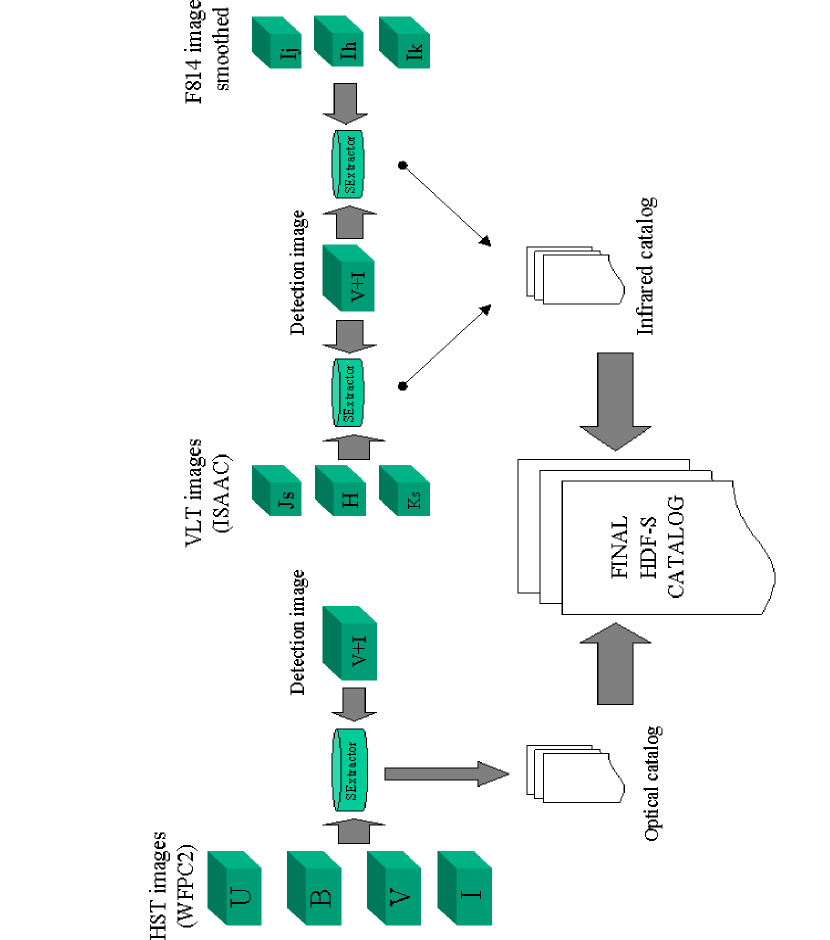
Figure 1: Global scheme of reduction.

Figure 1 shows the global scheme of the reduction.

3.1 Object Detection

The catalog was produced using the Source Extractor package (SExtractor Bertin & Arnouts 1996) in a slightly modified and more flexible version (see below).

Source detection and deblending were carried out on the inverse-variance-weighted sum of the $V$ and $I$ drizzled images. While other techniques for weighting are possible (e.g. Szalay et al. 1999), for most sources this summed image provides the maximum limiting depth. The resulting source position and isophotes are then used for subsequent photometric analysis in each of the individual bands. The combined $V+I$ image is significantly deeper than any of the individual images, and using it to define the object catalog allows, in practice, the detection of all the objects with “normal” SEDs that are detectable in the individual optical bands.

Source detection with SExtractor follows a standard “connected pixel” algorithm. To identify sources, the detection image is first convolved with a fixed smoothing kernel, for which we use a circular Gaussian with FWHM = 2.5 pixels. Pixels with convolved values higher than a fixed threshold are marked as potential sources. This threshold is in unit of $\sigma_{sky}$, where $\sigma_{sky}$ as a function of position comes from the background RMS map produced by SExtractor. The variation of S/N as a function of position is thus automatically taken into account.

After thresholding, regions consisting of more than a certain number of contiguous pixels are counted as sources. The aim of the present work is to provide a high-quality photometric catalog, sampling the SEDs of the sources from the UV to the NIR, in order to produce reliable photometric redshifts. Therefore we used a “conservative” detection strategy: the source detection threshold was set to 1.26 $\sigma_{sky}$ (per pixel in the convolved image) and the minimum area to 16 drizzled pixels, i.e. 0.025 square arcsec. After extensive tests of SExtractor it became clear that no single set of input parameters provides the desired detection depth for isolated objects and faint companions of bright galaxies, and the required rejection of spurious sources in correspondence with stellar diffraction spikes . This is a standard problem with SExtractor and at the moment an ideal solution does not exist. For example, Casertano et al. (2000) ran SExtractor two times with different detection thresholds. Objects from the deeper catalog are selectively removed and substituted with the corresponding ones from the shallower catalog. In this way, however, it is not easy to achieve consistent estimates of the fluxes (and in general also of the colors) with the different thresholds. Moreover the use of different detection thresholds can lead to the loss of objects near bright sources.

In order to obtain the desired detection depth and at the same time the required rejection of spurious sources with a single value of the detection threshold we introduced a modification of SExtractor that makes the detection strategy more flexible. To solve particular cases of clearly wrong detection (as described above), a table is prepared in which it is possible to define different values of the parameters in different regions of the frame (in the present application the $deblend$_$mincont$, the minimum contrast parameter for deblending, and the $detect$_$minarea$, the minimum number of pixels above threshold triggering detection ). Outside the specified subframes the program uses the $global$ parameters defined in the standard configuration file. In our case the global values are: $detect$_$minarea$ = 16 drizzled pixels and $deblend$_$mincont$ = 0.02. Therefore in a single run we obtained a unique catalog where all objects are detected over the same threshold ($detect$_$thresh$, the detection threshold). We defined 78 rectangular subframes, 57 with $deblend$_$mincont$ ranging from 0. to 1. (maximum deblending and no deblending) and the others with suitable $detect$_$minarea$ basically to avoid spurious detections. It is also possible to personalize both parameters at the same time in a given subframe, and define more subframes one inside the other.

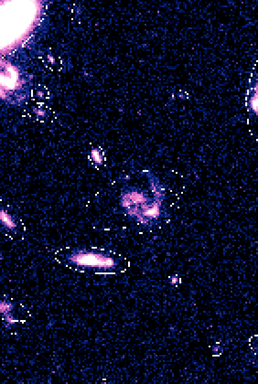
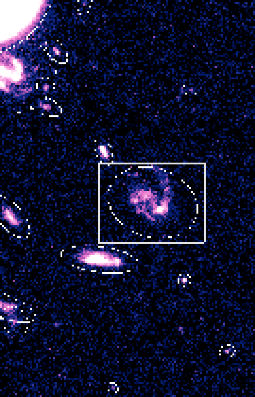
Figure 2: Left panel, detection without subframes, global parameter $deblend$_$mincont$=0.02. In the right panel detection with modified version of SExtractor, inside the rectangle $deblend$_$mincont$=1.0.

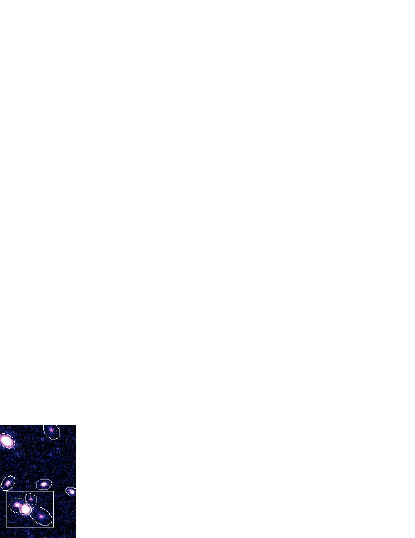
Figure 3: Left panel detection without subframes, global parameters $deblend$_$mincont$=0.02. In the right panel detection with modified version of SExtractor, inside the rectangle $deblend$_$mincont$=0.0004 (the coordinates X,Y of brighter object split are more accurate).

Although such a procedure is in direct contrast to the convenience of a fully automated algorithm able to process a large amount of data, we had to resort to it in order to ensure the highest quality of the result. In Figures 2,3 we show two examples of correction through the definition of subframes. The accurate detection is also helpful for the correct estimation of the object coordinates (X,Y) on the $V+I$ image. The correct centering of the photometric apertures is in fact a critical issue for the estimation of the colors, when SExtractor is used in $double$ $image$ $mode$ (see below).

The final result of the detection procedure is a list of 1611 objects.

The remaining process to obtain the photometry followed the standard SExtractor package.

3.2 Magnitudes

3.2.1 Optical catalog

To estimate the total magnitudes ($f(I)_{tot}$) of the objects, we used a procedure described by Djorgovski et al. (1995). For brighter objects, where the isophotal area (detected in $V$+$I$ image) is larger than 0.497 square arcsec (corresponding to an aperture of 20 pixels in diameter), we used the SExtractor $best$ magnitude as defined in the SExtractor manual. The $best$ magnitude is provided by an adaptive aperture method (mag $auto$), except if a neighbor is suspected to bias the measurement by more than 0.1 mag. In the latter case, the corrected isophotal magnitude is taken (Bertin & Arnouts, 1996).

For objects with an isophotal area smaller than 0.497 square arcsec, a magnitude estimated in a circular aperture of 0.8 arcsec (corresponding roughly to 5 FWHM) was used, corrected to the total $best$ magnitude provided by SExtractor, assuming that the wings follow a stellar profile. The corrections turned out to be independent of the magnitude and in terms of fluxes correspond to 1.061, 1.012, 1.010, 1.012 in the $U$, $B$, $V$ and $I$ band, respectively. There are 231 objects (out of 1611) with isophotal area greater than 0.497 square arcsec. The flux $best$ was computed (by SExtractor) for 208 objects out of 231 as a flux $auto$ and for the remaining 23 as isophotal corrected. These 23 objects are smoothly distributed in the range $22<I_{AB}<25$ and the RMS difference with respect to the flux $auto$ is 0.07 magnitudes.

We selected the $I$ as the fundamental band, and we referred to it for the determination of the object colors. If not otherwise specified, magnitudes are expressed in the AB system, that is a system based on a spectrum which is flat in $f_{\nu}$: $m=-2.5Logf_{\nu}+48.59$ (Oke, 1974).

In order to apply the photometric redshift codes it is mandatory to obtain a reliable estimation of the colors for each object. The colors were measured using the same fixed aperture (0.8 arcsec) in the different optical filters.

For the $U$, $B$, $V$ bands the flux is obtained by first estimating the ratio of the flux in each band with respect to the $I$ band within the same fixed aperture and then rescaling it to the total $I$ flux:

$$F(n)=[{f(n)\over f(I)}]_{fix.aperture}\times f(I)_{tot}$$ (1)

with $n$ = $U$, $B$, $V$. The corresponding error is estimated by standard propagation.

We ran SExtractor in the so-called $double$ $image$ $mode$: the $V$+$I$ image was used for the detection of the sources and the images in the bands $U$, $B$, $V$, $I$ for the photometric measurements.

3.2.2 Infrared catalog

The infrared frames have different orientation, pixel size and Point Spread Function (PSF) with respect to the HST images. In order to determine the color indices between the optical (in particular the $I$ band) and the near infrared bands ($Js$, $H$, $Ks$) we adopted the following strategy:

1. The IR images were rebinned to the same pixel size and orientation as the WFPC2 images.

2. To estimate colors, the $I$ frame was smoothed in turn to the same effective PSF of each of the images $Js$, $H$, $Ks$ (seeing $\simeq$ 0.6 arcsec) using a Fast Fourier Transform (FFT) approach.

   In order to obtain the correct transfer function, we extracted the median stellar PSF (obtained from 13 stellar objects) from each IR image and from the $I$ image, and we transformed them in the frequency space through a Fast Fourier Transform.

   The division of the FFTs of the infrared PSFs ($Js$, $H$, $Ks$) by the FFT of the $I$-band PSF provided the transformed transfer functions (i.e. the Fourier transform of the kernel). For each band, we inverse-transformed it in order to obtain the shape of the filter to be applied to the $I$ image (in the coordinates domain). The noise due to the presence of the aliasing frequencies in the Fourier space was reduced with a suitable filter. The flux is preserved.

   At the end we obtained three $I$-band smoothed images with the “same” PSF as the infrared images, namely: $I_{j}$, $I_{h}$, $I_{k}$.

3. We ran SExtractor in $double$ $image$ $mode$ with the detection in the $V$+$I$ image, and the photometry on the three smoothed $I$ band images ($I_{j}$, $I_{h}$, $I_{k}$) and on the three infrared images $Js$, $H$, $Ks$. We then computed the $I_{j}-Js$, $I_{h}-H$ and $I_{k}-Ks$ using a fixed aperture of $2\times FWHM$ diameter.

The estimated flux for each IR band is, again:

$$F(n)=[{f(n)\over f(In)}]_{fix.aperture}\times f(I)_{tot}$$ (2)

where $n$ runs over $Js$, $H$, $Ks$, and $[{f(n)\over f(In)}]_{fix.aperture}$ is the ratio of the flux in each IR band with respect to the $I$ smoothed image within the same fixed aperture. The $f(I)_{tot}$ is the total $I$ magnitude obtained as described in Sect. 3.2.1.

SExtractor was used (in $double$ $image$ $mode$) to carry out the photometry on all the objects detected in the $V+I$ image. The fraction of isolated objects that are not significantly detected in the IR images can be identified by comparing their fluxes with the corresponding errors.

There are however 317 sources (but only 7 with $K_{AB}<24$) for which a spurious IR flux is generated by contamination from a nearby brighter object. Those cases were identified on the basis of the optical images (using the $f(I)_{tot}/f(I_{n})$ ratio) and flagged as upper limits (see the description of the flag $f_{we}$ below).

3.3 Photometric errors for the infrared images

Because neighboring pixels are strongly correlated, the noise in the ISAAC images is not well described by the background RMS map produced by SExtractor, resulting in unrealistic estimates of the photometric uncertainties. In order to determine the correction factor to the errors provided by SExtractor we adopted the following strategy.

Synthetic stellar objects with known magnitude were generated with a relatively high signal to noise ratio (S/N = 20) and randomly inserted in 35 different relatively isolated regions of the frame. Their fluxes were then measured again with SExtractor. The dispersion in magnitude provides a reliable estimate of the real error which was used to rescale the formal SExtractor errors by a constant factor (3.25 in the three bands Js, H ,Ks).

4 The Catalog

The catalog is presented in Table 3.

For each object in the catalog we report the following parameters:

ID: The identification number. The objects in the list are sorted by increasing right ascension.

x, y: Abscissa and ordinate in pixels of the objects in the version 2 WFPC2 images.

RA, DEC: Coordinates RA and DEC (J2000) in the version 2 WFPC2 images.

$m_{i}$ and $\sigma(m_{i})$: The magnitude in the $I$ image and its uncertainty. It is the $best$ SExtractor magnitude if the isophotal area of the object is greater then 0.497 square arcsec (314 pixel), otherwise it is the fixed aperture magnitude (diameter 0.8 arcsec).

flux and $\sigma$ (flux): The aperture fluxes, with their uncertainties (for the IR images they were estimated according to the procedure described in Sect. 3.2.2).

s/g: The star-galaxy separation provided by SExtractor applied to the $V$+$I$ image to which the best PSF corresponds. This classifier gives output values in the range (0-1) (0 for galaxies and 1 for stars) and represents the degree of membership of an object to one of the two classes.

$f_{s}$: The internal flag provided by SExtractor (see Bertin & Arnouts 1996). It is a short integer containing, coded in decimal, all the extraction flags as a sum of powers of two:

• 1 - The object has neighbors, bright and close enough to significantly bias the photometry, or bad pixel.

• 2 - The object was originally blended with another one.

• 4 - At least one pixel of the object is saturated (or very close to).

• 8 - The object is truncated (too close to an image boundary).

• 16 - Object’s aperture data are incomplete or corrupted.

• 32 - Object’s isophotal data are incomplete or corrupted.

• 64 - A memory overflow occurred during deblending.

• 128 - A memory overflow occurred during extraction.

$f_{we}$: Flag for infrared fluxes, for the eventual contamination of the flux estimation from neighboring objects. In these cases the flux measurement is considered as an upper limit. The coding is a sum of powers of 2 (ranging from 0 to 7): for example 7 corresponds to 111 in binary and means that the infrared fluxes in $Js$, $H$, $Ks$ are all upper limits, 4 (100) only the $Js$ band is an upper limit, 3 (011) both $H$ and $Ks$ bands are upper limits, 0 (000) all fluxes in the infrared bands have been measured without problems, etc.

5 Discussion

5.1 Source Counts

Figure 4 shows the behavior of the observed source counts: the result of the present work is consistent with the corresponding estimates in the HDF-S of Casertano et al. (2000) down to $I_{AB}$ $\sim$ 28 and with the counts in the HDF-N by Williams et al. (1996). On the other hand, if we compare our source counts with the result in the HDF-N by Fernández-Soto et al. (1999), beyond $I_{AB}$ $\sim$ 26 the HDF-N counts turn out to be systematically lower with respect to the HDF-S by about a factor 1.5, while the source counts in the HDF-S by Volonteri et al. (2000) appear to be higher in this range by about the same factor. These discrepancies are to be ascribed to differences in the approach used to carry out the photometry, in particular the profile fitting method for Fernández-Soto et al. (1999) and different parameters for the source detection in the case of Volonteri et al. (2000).

In order to compute the incompleteness of the source counts two different approaches were followed, with the aim of obtaining an estimate of the systematic uncertainties. In the first method 46 galaxies in the magnitude interval $24.5<I_{AB}<25$ were selected and their extracted $V+I$ images were randomly inserted in the $V+I$ WF image, suitably dimmed by increasing factors in order to cover the magnitude range down to $I_{AB}=28$. Then the source detection was performed with the same SExtractor parameters used in the original image. For each 0.5 magnitude bin 30 simulations were carried out. The resulting incompleteness is listed in Col.3 ($c_{gal}$) of Table 4. For the magnitude bins brighter than $I_{AB}=24.5$ no simulations were carried out and the incompleteness factor corresponds to the masked area due to the brightest objects in the field (see Sect.3.1).

The same approach was also applied using a reference sample of 46 stellar images, in order to estimate a lower limit of the incompleteness. The result is listed in Col.4 ($c_{star}$) of Table 4 and is increasingly different from the case of the galaxy simulations beyond $I_{AB}=26.5$.

The estimated surface density, corrected by the incompleteness factor for galaxies, is listed in Col.5 ($Nc_{gal}$) and is in very good agreement with the corrected source counts of Volonteri et al. (2000).

Fig. 5 shows the extragalactic background light (EBL) per half magnitude bin, $i_{\nu}=10^{-0.4(I_{\rm AB}+48.6)}N(I_{\rm AB})$, as a function of $I$ magnitude. The agreement with the work of Madau & Pozzetti (2000) is very good down to $I_{AB}\simeq 26$. Beyond this limit the Madau & Pozzetti (2000) values are close to our estimates corrected by the incompleteness factor for stars rather than for galaxies. In any case the uncertainty of this correction has little effect on the total amount of EBL in $I$. Adopting the values of Madau & Pozzetti (2000) down to $I_{AB}=22$ and our counts at fainter magnitudes, the EBL in the $I$ band turns out to be $8.7$ and $8.8$ nW m^-2 sr^-1 using the incompleteness correction for stars and galaxies, respectively. These values are well within the uncertainty of the estimate by Madau & Pozzetti (2000), $8.04_{-0.92}^{+1.62}$ nW m^-2 sr^-1, which arises mostly from field-to-field variations in the number of relatively bright galaxies.

5.2 Colors

In Figure 6 we show the comparison between the optical colors of our catalog as a function of the $I_{AB}$ magnitude and those obtained by Casertano et al. (2000). The objects were selected with the magnitude $U$, $B$, $V$, $I$ brighter than 27.0, 27.5, 27.5, 27.5 respectively. The main differences (in particular in the $U$ band) are due to the different strategy adopted in terms of detection and photometry: we computed the colors using a fixed aperture, while Casertano et al. (2000) computed the isophotal colors.

The comparison between the colors of the HDF-S (our catalog) and HDF-N (Fernández-Soto et al. 1999) is shown in Figure 7. There is a significant difference in the median color $V-I$ between the HDF-S and the HDF-N around magnitude $I_{AB}$ $\sim$ 26. This could be due to systematic differences in the distributions of the galaxy redshifts in the two fields, in particular to the presence of large scale structure at $z\sim 1$ (Cohen et al., 2000) and will be discussed in a forthcoming paper. Beyond $I_{AB}$=28 the limited depth of the V image (29.5, 2$\sigma$) gives rise to systematic effects in the color $V$-$I$.

Color criteria, which are sensitive to the presence of a Lyman continuum break superposed on an otherwise flat UV spectrum, have been shown to successfully identify high redshift star-forming galaxies (e.g. Madau et al. 1996). In Figure 8 we show the selection of $U$-band dropouts with $I_{AB}<27$ (according to the criteria defined by Madau et al. 1996). The dashed lines outline the selection region within which candidate $2.5<z<3.5$ objects are identified. Objects undetected in the $U$ band (with signal-to-noise $<$ 1) are plotted as triangles at the 1$\sigma$ limits to their $(U-B)_{AB}$ colors. We adopted a similar technique to select candidate $3.5<z<4.5$ galaxies with $I_{AB}<27$ (see Figure 9). The selection area is outlined with dashed lines. The undetected objects in the $B$ band (with signal-to-noise $<$ 1) are plotted as triangles. Symbol sizes scale with the $I_{AB}$ magnitude of the object.

90 $U$-band dropouts and 17 $B$-band dropouts are identified, equivalent to a surface density of $(21\pm 1)$ and $(3.9\pm 0.9)$ per square arcmin, respectively. They are listed in Table 5 and Table 6.

5.3 Extremely Red Objects

The selection of Extremely Red Objects (EROs) is shown in Figure 10 (upper panel). EROs are defined as sources with $(I-K)_{AB}>2.7$, corresponding to the color of passively evolving elliptical galaxies at $z>1$. The selection was carried out down to $K_{AB}<24$. Table 7 lists the ID number and coordinates of 11 EROs in the field (plus 3 more objects whose upper limit to the Ks flux is still compatible with the selection criterion).

Saracco et al. (2001), using the same infrared images as the present work, selected 20 EROs on the basis of a color criterion $Js-Ks>2.4$, corresponding to a surface density of 2.7 per square arcmin. Ten of these EROs lie in the area covered by our multicolor catalog and six of them were selected with the above-described $(I-K)_{AB}>2.7$ threshold. In the catalog of Saracco et al. (2001) there is only one object detected with a S/N$>5$ in the $Ks$ band that is not present in our catalog.

This object is clearly seen in the $Ks$ image, while no optical counterpart is present in the $I$ band. It is marked in Figure 10 with an upward-pointing arrow as a 5$\sigma$ lower limit at $I_{AB}$$\sim$28 and listed in Table 7 with the ID 9999. Adding this object to our sample the EROs surface density turns out to be $(3.2\pm 0.9)$ per square arcmin, $(2.5\pm 0.8)$ per square arcmin without the 3 upper limits in the Ks band.

The EROs surface density measured in the present work is similar to the result obtained by Saracco et al. (2001) in the same HDF-S field (but over a larger area). On the other hand the surface density observed by Saracco et al. (2001) in the Chandra Deep Field (Giacconi et al., 2001, CDF) is significantly different ($1.2\pm 0.5$ per square arcmin). The discrepancy between the two fields is probably due to the clustering properties of EROs associated to the relatively small field of CDF and HDF-S. Daddi et al. (2000) detect a strong clustering signal of EROs, selected on the basis of the $R-K$ color from a $K_{\rm Vega}$ $\sim$ 19 limited sample in a wide area of $\sim$ 25 square arcmin. We select EROs on a sample 3 magnitudes fainter and with different color criteria. Thus, the results of Daddi et al. (2000) cannot be directly applied to our data. Nevertheless, the distribution of EROs in the HDF-S field is not uniform: there are 10 EROs (2 of them are upper limits in the Ks band) inside the upper WFPC2 chip.

In the EROs sample there is an interesting radio source identified and discussed by Norris et al. (1999) which has an $(I-Ks)_{AB}$= 3.45. This object is unusual in that its radio-optical ratio is about 1000 times higher than that of any galaxy known in the local Universe.

We adopted the photometric criterion of Pozzetti & Mannucci (2000) to distinguish between the two EROs populations of ellipticals and starbursts. In doing so we assume that our EROs sample belongs to the redshift range of applicability of the criterion, $1<z<2$. While an old stellar population is characterized by sharp breaks (especially around 4000Å), young dusty galaxies show shallower SEDs in the rest-frame optical part of the spectrum because dust extinction does not produce sharp breaks. It is possible to measure the steepness of the SED for objects with $1<z<2$ using the observed J-K color. In the lower panel of the Figure 10 the I-K vs. J-K plane for the ERO sample is shown. The dashed line separating the elliptical from the starburst galaxies corresponds to: $J_{AB}-K_{AB}=0.36(I_{AB}-K_{AB})+0.045$.

The morphological selection of early-type galaxies is usually carried out by fitting a generalized de Vaucouleurs law ($\mu_{r}-\mu_{0}\propto(r/r_{e})^{1/n}$ to the luminosity profile of the objects, where $\mu_{r}$ is the surface brightness at the radius $r$, $r_{e}$ is the half light radius and $n$ is the Sersic index (Sersic, 1968). For elliptical galaxies $n>2$ (see, for example, Rodighiero, Franceschini & Fasano (2001)). In the present case, the EROs have typically $I_{AB}>26$ and except for the few brighter objects it is impossible to compute a reliable fit, even on the $V+I$ image. For the fainter EROs a rough morphological classification was carried out comparing the central intensity vs. the area of the images. A visual inspection of all the EROs was also carried out to check the results. In Table 7 the EROs are listed, according to their morphology, as early type ($E$, 3 objects), late type ($L$, 1 object) and objects too faint for a reliable classification ($S$, 11 objects). In the lower panel of Figure 10, the three ellipticals are marked with a cross inside the symbol, and the late-type galaxy is shown with a filled symbol. The other points belong to the (S) category. The classification obtained with the morphological method agrees with the photometric classification for the three ellipticals. The object morphologically classified as “late-type” corresponds to an IR upper limit and it is not clear whether it can be considered an ERO.

In the upper panel of Figure 10, the elliptical galaxies (according to the photometric classification) are marked with a star. About half of the EROs in the sample seem to belong to the “Starburst” category and, in general, show an $I-K$ color redder than the corresponding $I-K$ of the “Ellipticals”.

In Figures 11 and 12 the $V+I$ and Ks images of the ERO sample are shown.

It is worth noting that the above-mentioned radio galaxy (marked with a triangle in Figure 10) belongs to the “early-type” class according to the color-color separation technique. Rodighiero, Franceschini & Fasano (2001) also put it in a sample of “early-type” objects, estimating for this object a Sersic index $n\sim 2.2$ (G. Fasano, private communication) i.e. at the border of the early-/late-type discrimination.

Figure 4: Comparison between the object counts in the HDF-S and the HDF-N. The present catalog (HDF-S-2), Casertano et al. (2000) (HDF-S-1), Volonteri et al. (2000) (HDF-S-3); Fernández-Soto, Lanzetta K. M. & Yahil (1999) (HDF-N-2) and Williams et al. (1996) (HDF-N-1). All the samples, except the Volonteri et al. (2000), include the planetary camera.

Figure 5: The extragalactic background light per half magnitude bin, $i_{\nu}=10^{-0.4(I_{\rm AB}+48.6)}N(I_{\rm AB})$, as a function of $I$ magnitude. The open circles are taken from Madau & Pozzetti (2000). The filled circles were obtained in the present work adopting the incompleteness correction estimated for galaxies (see text). The error bars at $I_{AB}\simeq 26$ show the lower limit corresponding to the incompleteness correction estimated for objects with a stellar PSF.

Figure 6: Comparison of the magnitudes and colors estimated in the present work and the results of Casertano et al. (2000). In abscissa the magnitudes, in ordinate the differences between our estimates and those of Casertano et al. (2000).

Figure 7: Comparison between HDF-S and HDF-N (Fernández-Soto, Lanzetta K. M. & Yahil, 1999). In the first two panels the $V-I$ color versus $I$ (AB) is shown. The third panel shows the comparison between the median $V-I$ colors in 0.5 magnitude bins. Beyond $I_{AB}$=28 the limited depth of the V image (29.5, 2$\sigma$) gives origin to systematic effects on the $V$-$I$ color.

Figure 8: Color-color plot for the candidate U-band dropouts (above the dashed line) in the HDF-S. The size of the symbols scales with the magnitude in $I_{AB}$. There are two spectroscopic redshift available (from Cristiani et al. 2000).

Figure 9: Color-color plot for the candidate B-band dropouts (above the dashed line) in the HDF-S. The size of the symbols scales with the magnitude in $I_{AB}$.

Figure 10: EROs in the HDF-S ($(I-K)_{AB}>2.7$ and $K_{AB}<24$). In the upper panel empty symbols indicate the $Starburst$ galaxies and the stars the $Ellipticals$. The triangle corresponds to a radio-galaxy (see text). In the upper panel the error bars are plotted in the upper left corner for an object with $K_{AB}$ = 24 and $(I-K)_{AB}$ = 3.5. In the lower panel the classification between $Elliptical$ and $Starburst$ is carried out with a color-color technique (Pozzetti et al. 2000). Crosses indicate objects morphologically classified as elliptical galaxies. The filled circle in both panels is an object morphologically classified as “late-type”.

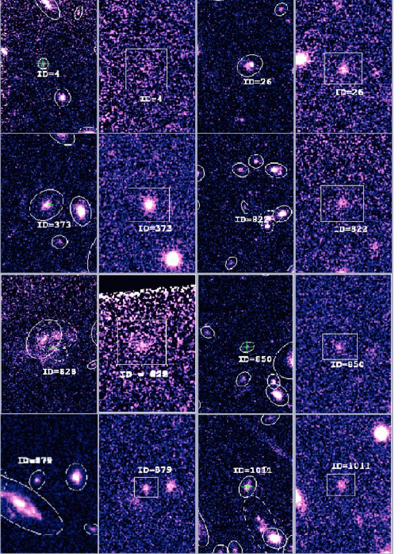
Figure 11: EROs in the $V+I$ and $Ks$ images, they are marked with a cross and the identifier.

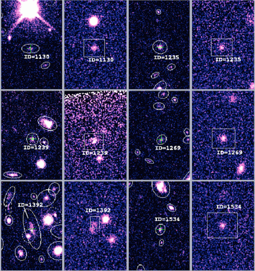
Figure 12: EROs in the $V+I$ and $Ks$ images, they are marked with a cross and the identifier.

Table 1: WFPC2 observations

Filter	Number of	total	FWHM	Zero-point	Limiting AB Magnitude
	frames	time (s)	(arcsec)	ABMAG	(10-$\sigma$ in 0.2 square arcsec)
F300	102	132585	0.14	20.77	26.8
F450	51	101800	0.14	21.9	27.7
F606	49	97200	0.14	23.02	28.3
F814	56	112200	0.14	22.09	27.7

Table 2: ISAAC observations

Filter	$<\lambda>$	$\Delta\lambda$	Number of	total	FWHM	Zero-point	Limiting Magnitude
			frames	time (s)	(arcsec)		5-$\sigma$
Js	1.24	0.16	210	25200	0.60	28.35	23.5
H	1.65	0.30	181	21720	0.60	27.50	22.0
Ks	2.16	0.27	487	29220	0.60	26.26	22.0

Table 3: The object catalog for the HDF-S WFPC2 field

ID	x	y	$\alpha(22^{h}:m:s)$	$\delta(-60^{\circ}:^{\prime}:^{\prime\prime})$	$m_{i}$	$\sigma(m_{i})$	Flux $U$	$errU$	Flux $B$	$errB$	Flux $V$	$errV$	Flux $J$	$errJ$	Flux $H$	$errH$	Flux $K$	$errK$	s/g	$f_{s}$	$f_{we}$
1	222.56	1849.99	33 05.771	33 23.32	27.08	0.11	0.0144	0.0079	0.0312	0.0039	0.0382	0.0024	0.3045	0.2701	0.1359	0.4970	0.2725	0.4323	0.01	0	0
2	229.87	1667.82	33 05.728	33 30.57	29.72	1.29	0.0009	0.0091	-0.0032	0.0041	0.0071	0.0024	0.1733	0.1826	-0.0959	0.3911	-0.1325	0.3180	0.53	0	7
3	245.78	1812.88	33 05.647	33 24.79	27.75	0.19	0.0210	0.0076	0.0131	0.0038	0.0140	0.0023	-0.0406	0.2279	0.2266	0.4699	0.3363	0.4302	0.20	0	0
4	248.01	2109.94	33 05.647	33 12.95	28.08	0.34	0.0080	0.0096	0.0015	0.0046	0.0153	0.0027	-0.0589	0.2563	0.5490	0.8582	0.9603	1.2918	0.88	0	0
5	252.54	2205.65	33 05.625	33 09.13	26.00	0.09	0.0149	0.0126	0.0727	0.0065	0.0903	0.0035	0.2667	0.1143	0.4916	0.2870	-0.1419	0.1902	0.03	0	0

Note. — From Casertano et al. 2000.

Note. — Magnitudes are provided in the Vega magnitude system.

Note. — Fluxes and corresponding errors are in units of $10^{10}\rm{erg~{}cm^{-2}~{}s^{-1}~{}Hz^{-1}}$.

The complete version of this table is in the electronic edition of the Journal. The printed edition contains only a sample.

Table 4: Counts in the F814W band measured in the inner area of the WF camera ($4.49$ arcmin² in the present work, $4.38$ arcmin² in the work of Volonteri et al. (2000)).

$I_{AB}$	$n$	$c_{gal}$	$c_{star}$	$Nc_{gal}$	$Nc_{star}$	$n_{vol}$	$c_{vol}$	$Nc_{vol}$
				($0.5~{}mag^{-1}$	($0.5~{}mag^{-1}$			($0.5~{}mag^{-1}$
				$arcmin^{-2}$)	$arcmin^{-2}$)			$arcmin^{-2}$)
22.25	11	1.04	1.04	2.55	2.55	11	1	2.51
22.75	17	1.04	1.04	3.94	3.94	28	1	6.39
23.25	25	1.04	1.04	5.79	5.79	26	1	5.94
23.75	28	1.04	1.04	6.49	6.49	35	1	7.99
24.25	35	1.04	1.04	8.11	8.11	37	1	8.45
24.75	53	1.04	1.04	12.28	12.28	65	1	14.84
25.25	46	1.05	1.05	10.76	10.76	94	1	21.46
25.75	79	1.07	1.06	18.83	18.65	139	1	31.73
26.25	143	1.11	1.06	35.35	33.76	173	1	39.50
26.75	157	1.23	1.07	43.01	37.41	235	1	53.65
27.25	205	1.59	1.08	72.59	49.31	342	1.08	84.33
27.75	222	2.87	1.12	141.90	55.38	332	1.86	140.99

Table 5: HDF-S U-dropouts

ID	IAB	(B-I)AB	(U-B)AB	X	Y	RA	DEC
28	24.20	0.31	3.53	381.90	1663.84	22 33 04.90	-60 33 30.7
46	26.26	0.26	2.47	445.65	1420.50	22 33 04.55	-60 33 40.4
49	26.44	-0.01	2.53	456.64	1695.53	22 33 04.50	-60 33 29.4
56	24.88	0.83	2.90	479.55	1811.28	22 33 04.38	-60 33 24.8
57	26.59	0.42	1.96	489.72	1669.49	22 33 04.32	-60 33 30.4
80	25.34	0.73	2.37	565.62	1027.16	22 33 03.88	-60 33 56.0
81	24.30	0.56	2.20	565.77	2083.53	22 33 03.93	-60 33 13.9
89	25.90	-0.04	1.54	596.78	1023.16	22 33 03.71	-60 33 56.1
109	25.09	0.28	3.15	669.68	571.08	22 33 03.30	-60 34 14.1
115	23.25	0.68	2.16	695.55	1685.70	22 33 03.21	-60 33 29.7
124	25.41	0.58	2.54	727.14	1083.73	22 33 03.01	-60 33 53.7
127	25.46	1.10	2.46	736.19	965.96	22 33 02.96	-60 33 58.4
219	24.74	0.47	1.83	1137.10	1426.53	22 33 00.81	-60 33 39.9
225	25.98	0.76	2.25	1152.38	872.99	22 33 00.70	-60 34 02.0
307	25.69	0.21	1.82	1402.15	1216.71	22 32 59.37	-60 33 48.2
329	26.16	-0.16	2.23	1457.20	1077.04	22 32 59.06	-60 33 53.7
382	25.98	0.54	2.50	1567.01	1102.02	22 32 58.47	-60 33 52.7
385	25.54	0.49	3.00	1570.16	1127.06	22 32 58.46	-60 33 51.7
396	24.74	0.74	2.86	1604.91	1695.32	22 32 58.29	-60 33 29.0
536	26.08	0.10	1.90	1986.10	907.38	22 32 56.20	-60 34 00.3
540	26.05	-0.02	1.66	1989.17	620.40	22 32 56.17	-60 34 11.7
583	24.87	0.60	3.29	2072.45	3106.80	22 32 55.83	-60 32 32.6
600	26.72	0.33	1.88	2124.12	4053.40	22 32 55.60	-60 31 54.8
638	26.09	0.46	1.88	2213.60	1214.37	22 32 54.98	-60 33 48.0
646	26.38	0.36	2.15	2229.45	1710.16	22 32 54.92	-60 33 28.2
649	25.70	-0.10	3.28	2234.97	1359.88	22 32 54.87	-60 33 42.2
663	26.74	0.05	1.55	2268.45	1293.80	22 32 54.69	-60 33 44.8
676	26.11	0.24	1.93	2290.75	2716.97	22 32 54.63	-60 32 48.1
685	25.80	0.87	2.32	2308.56	2887.93	22 32 54.54	-60 32 41.2
693	26.34	-0.06	1.42	2322.93	699.27	22 32 54.37	-60 34 08.5
709	26.82	0.23	1.63	2341.94	2472.97	22 32 54.35	-60 32 57.8
719	25.56	0.08	2.01	2354.33	2476.44	22 32 54.28	-60 32 57.6
723	24.56	0.56	2.25	2359.55	682.90	22 32 54.16	-60 34 09.1
738	25.30	0.72	2.63	2387.22	3168.21	22 32 54.13	-60 32 30.1
757	26.57	0.39	1.93	2415.28	904.51	22 32 53.88	-60 34 00.3
776	25.85	0.46	2.67	2447.00	4070.66	22 32 53.85	-60 31 54.0
778	26.22	0.10	1.84	2450.30	967.91	22 32 53.69	-60 33 57.7
784	26.31	0.71	1.98	2455.43	3453.57	22 32 53.78	-60 32 18.7
802	24.54	1.05	2.77	2507.67	2110.67	22 32 53.43	-60 33 12.2
807	24.67	0.94	2.32	2512.53	3856.67	22 32 53.49	-60 32 02.5
829	25.03	0.79	2.44	2544.12	1906.26	22 32 53.23	-60 33 20.3
847	26.60	0.28	1.59	2571.80	4045.39	22 32 53.18	-60 31 55.0
855	26.41	0.03	2.47	2582.79	4120.85	22 32 53.12	-60 31 52.0
868	26.94	-0.01	1.96	2606.04	1104.37	22 32 52.85	-60 33 52.2
870	26.33	0.15	1.82	2606.41	1228.31	22 32 52.86	-60 33 47.3
871	24.89	0.74	3.19	2606.45	1869.42	22 32 52.89	-60 33 21.7
913	26.92	0.13	1.92	2676.51	2941.20	22 32 52.56	-60 32 39.0
914	25.62	0.56	2.58	2681.97	2405.91	22 32 52.51	-60 33 00.3
949	25.26	0.49	2.15	2740.41	2984.83	22 32 52.21	-60 32 37.2
957	24.66	1.05	2.96	2759.70	1344.73	22 32 52.03	-60 33 42.6
960	26.62	-0.02	2.00	2765.76	2729.73	22 32 52.07	-60 32 47.4
968	26.68	0.23	1.96	2778.16	4205.43	22 32 52.08	-60 31 48.6
991	26.69	0.54	1.76	2808.66	3222.52	22 32 51.86	-60 32 27.7
992	24.48	1.12	2.76	2808.81	3768.18	22 32 51.89	-60 32 06.0
1007	26.54	0.53	1.94	2834.69	3331.53	22 32 51.72	-60 32 23.4
1025	25.06	0.42	2.93	2874.27	2037.31	22 32 51.45	-60 33 14.9
1068	26.94	0.23	1.50	2938.20	3806.90	22 32 51.19	-60 32 04.4
1081	26.99	0.38	1.64	2964.56	3705.72	22 32 51.04	-60 32 08.4
1100	23.32	0.75	1.97	3012.83	1694.70	22 32 50.68	-60 33 28.6
1123	26.43	0.19	1.87	3052.65	3719.02	22 32 50.57	-60 32 07.9
1149	25.91	0.50	2.50	3091.54	2122.05	22 32 50.28	-60 33 11.5
1167	25.93	0.30	2.66	3121.38	1434.79	22 32 50.08	-60 33 38.9
1174	24.14	0.81	2.85	3125.97	985.42	22 32 50.04	-60 33 56.8
1179	25.84	0.27	1.85	3137.28	3750.66	22 32 50.11	-60 32 06.6
1196	26.90	0.19	1.84	3175.93	1894.17	22 32 49.81	-60 33 20.5
1204	26.42	-0.09	1.96	3197.90	1817.71	22 32 49.69	-60 33 23.6
1212	25.04	0.12	1.93	3211.36	2333.12	22 32 49.64	-60 33 03.0
1225	25.54	0.67	2.66	3234.36	826.16	22 32 49.45	-60 34 03.1
1232	25.69	0.37	2.33	3256.86	3861.56	22 32 49.47	-60 32 02.1
1242	22.92	0.66	3.57	3265.10	3254.94	22 32 49.40	-60 32 26.3
1249	26.24	0.27	2.43	3271.88	1251.97	22 32 49.26	-60 33 46.1
1261	25.90	0.59	2.45	3288.07	2844.31	22 32 49.26	-60 32 42.6
1277	23.28	0.69	3.76	3305.11	3261.82	22 32 49.18	-60 32 26.0
1281	26.86	0.00	1.48	3316.19	2780.19	22 32 49.09	-60 32 45.2
1303	25.13	0.43	2.72	3350.99	3022.72	22 32 48.92	-60 32 35.5
1322	25.52	0.16	1.62	3401.43	2983.13	22 32 48.65	-60 32 37.0
1372	25.79	0.92	2.26	3459.33	3083.83	22 32 48.34	-60 32 33.0
1374	26.44	0.45	1.73	3469.88	3413.81	22 32 48.30	-60 32 19.9
1397	24.86	0.83	2.32	3508.06	2171.68	22 32 48.03	-60 33 09.4
1411	26.56	0.28	2.07	3529.57	1963.53	22 32 47.90	-60 33 17.6
1414	26.69	0.21	1.64	3533.03	3549.59	22 32 47.97	-60 32 14.4
1432	24.22	0.78	2.49	3562.83	3420.07	22 32 47.80	-60 32 19.6
1452	25.94	0.65	2.32	3589.04	3993.43	22 32 47.68	-60 31 56.7
1457	26.02	0.26	2.62	3599.39	1368.64	22 32 47.50	-60 33 41.3
1466	25.86	0.36	2.53	3618.27	2690.07	22 32 47.46	-60 32 48.6
1523	25.51	0.33	2.43	3721.70	2488.36	22 32 46.89	-60 32 56.7
1524	26.09	0.08	1.89	3725.12	2092.66	22 32 46.85	-60 33 12.4
1532	26.38	0.08	2.37	3740.41	2895.03	22 32 46.81	-60 32 40.4
1572	26.92	0.29	1.56	3830.48	1300.51	22 32 46.25	-60 33 44.0
1588	24.95	0.41	1.98	3883.97	1288.26	22 32 45.95	-60 33 44.4

Note. — $n$ and $n_{vol}$ are the observed counts in 0.5 magnitude bins in the present work and in the catalog by Volonteri et al. (2000), respectively. $c_{gal}$ and $c_{star}$ are the incompleteness correction factors derived from our simulations for galaxies and stars, respectively (see text). $Nc_{gal}$ and $Nc_{star}$ are the corrected counts derived in the present work adopting the incompleteness correction estimated for galaxies and for stars, respectively. $c_{vol}$ is the incompleteness correction factor and $Nc_{vol}$ the corrected counts per square arcmin as estimated by Volonteri et al. (2000).

Note. — List of U-band dropout candidates.

Table 6: HDF-S B-dropouts

ID	IAB	(V-I)AB	(B-V)AB	X	Y	RA	DEC
36	26.79	0.20	1.71	397.39	1030.43	22 33 04.79	-60 33 55.9
209	26.38	0.84	2.25	1119.71	815.73	22 33 00.88	-60 34 04.2
320	26.65	0.53	1.67	1425.84	1247.15	22 32 59.24	-60 33 46.9
344	26.47	0.19	1.84	1479.11	917.34	22 32 58.94	-60 34 00.1
369	26.08	0.74	2.59	1539.58	692.30	22 32 58.60	-60 34 09.0
442	26.31	0.20	1.82	1745.15	1205.75	22 32 57.51	-60 33 48.5
627	26.97	0.23	1.68	2196.19	2326.58	22 32 55.13	-60 33 03.6
721	26.89	0.66	2.36	2358.17	2817.65	22 32 54.27	-60 32 44.0
892	25.77	0.82	3.12	2653.70	2543.59	22 32 52.67	-60 32 54.8
897	27.00	0.55	2.39	2659.16	3657.16	22 32 52.69	-60 32 10.5
1004	26.22	0.73	2.29	2831.33	2109.59	22 32 51.69	-60 33 12.1
1144	26.43	0.93	2.50	3084.84	2152.57	22 32 50.32	-60 33 10.3
1151	26.79	0.60	2.43	3093.98	2959.69	22 32 50.30	-60 32 38.1
1155	26.23	0.14	1.69	3099.80	2050.02	22 32 50.23	-60 33 14.4
1400	26.53	0.77	2.26	3516.67	3877.74	22 32 48.07	-60 32 01.4
1461	26.08	0.46	2.03	3606.20	3451.91	22 32 47.56	-60 32 18.3
1494	26.38	0.76	2.72	3670.06	3641.84	22 32 47.23	-60 32 10.7

Note. — List of B-band dropout candidates.

Table 7: EROs

ID	RA	DEC	$K_{AB}$	$I_{AB}$	$(I-K)_{AB}$	Morphology
4	22 33 05.65	-60 33 12.90	23.63	28.08	4.44*	$S$
26	22 33 04.96	-60 33 22.20	22.89	26.15	3.26	$S$
373	22 32 58.60	-60 33 46.58	22.31	25.75	3.45	$E(Radio~{}Gal.)$
822	22 32 53.39	-60 31 54.33	23.39	28.11	4.72	$S$
828	22 32 53.34	-60 31 46.58	23.09	26.56	3.47*	$S$
850	22 32 53.01	-60 33 57.03	23.67	27.58	3.90	$S$
879	22 32 52.91	-60 32 15.72	23.71	26.81	3.10	$S$
1011	22 32 51.54	-60 33 58.40	23.35	26.21	2.87	$S$
1130	22 32 50.49	-60 32 22.64	23.23	26.89	3.66	$S$
1235	22 32 49.46	-60 31 57.88	23.45	26.21	2.76	$E$
1239	22 32 49.46	-60 31 46.58	22.70	26.25	3.55	$E$
1269	22 32 49.25	-60 32 11.62	22.93	27.06	4.13	$S$
1392	22 32 48.15	-60 32 17.47	23.52	26.35	2.83*	$L$
1534	22 32 46.79	-60 32 33.74	23.05	26.92	3.87	$S$
9999	22 32 55.92	-60 32 50.28	23.95	—	$>4$	$S$

References

- Bertin & Arnouts (1996) Bertin, E., Arnouts, S. 1996, A&A, 117, 393
- Casertano et al. (2000) Casertano, S., de Mello, D., Dickinson, M., Ferguson, H. C., Fruchter, A. S., Gonzalez-Lopezlira, R. A., Heyer, I., Hook, R. N., Levay, Z., Lucas, R. A., Mack, J., Makidon, R. B., Mutchler, M., Smith, T. E., Stiavelli, M., Wiggs, M. S., Williams, R. E., 2000, AJ, 120, 2747
- Cohen et al. (2000) Cohen, J. G., Hogg, D. W., Blandford, R., Cowie, L. L., Hu, E., Songaila, A., Shopbell, P., Richberg, K., 2000, ApJ, 538, 29
- Cristiani et al. (2000) Cristiani, S., Appenzeller, I., Arnouts, S., Nonino, M., Aragón-Salamanca, A., Benoist, C., da Costa, L., Dennefeld, M., Rengelink, R., Renzini, A., Szeifert, T., White, S., 2000, A&A, 359, 489
- Daddi et al. (2000) Daddi, E., Pozzetti, L., Hoekstra, H., Röttgering, H.J.A., Renzini, A., Zamorani, G., Mannucci, F., 2000, A&A, 361, 535
- Djorgovski et al. (1995) Djorgovski, S., Soifer, B. T., Pahre, M. A., Larkin, J. E., Smith J. D., Neugebauer, G., Smail, I., Matthews, K., Hogg, D. W., Blandford R. D., Cohen, J., Harrison, W., Nelson, J. 1995, ApJ, 438, L13
- Fernández-Soto, Lanzetta K. M. & Yahil (1999) Fernández-Soto, A., Lanzetta, K.M., Yahil, A., 1999, ApJ, 513, 34
- Fruchter et al. (2001) Fruchter, A., Bergeron, L. E., Dickinson, M., Ferguson, H. C., Hook R. N., et al. 2001, in preparation
- Gardner et al. (2000) Gardner, J., Baum, S. A., Brown, T. M., Carollo, C. M., Christensen, J., et al. 2000, AJ, 119, 486
- Giacconi et al. (2001) Giacconi R., Rosati P., Tozzi P., Nonino M., Hasinger G., Norman C., Bergeron J., Borgani S., Gilli R., Gilmozzi R., Zheng W., 2001, ApJ, 551, 624
- Madau et al. (1996) Madau, P., Ferguson, H. C., Dickinson, M., Giavalisco, M., Steidel, C. C., Fruchter, A. S. 1996, MNRAS, 283, 1388
- Madau & Pozzetti (2000) Madau, P., Pozzetti, L., 2000, MNRAS, 312, L9
- Moorwood et al. (1999) Moorwood, A.F.M., Cuby, J.G., Ballester, P., et al., 1999 , The ESO Messenger 95, 1
- Norris et al. (1999) Norris, R. P., Hopkins, A., Sault, R. J., Ekers, R. D., Ekers, J., Badia, F., Higdon, J., Wieringa, M.H., Boyle, B.J., Williams R. E., astro-ph/9910437
- Oke (1974) Oke J.B. 1974, ApJS, 27, 21
- Persson et al. (1998) Persson, E., Murphy, D. C., Krzeminski, W., Roth, M., Rieke, M. J., 1998, AJ, 166, 2475
- Pozzetti & Mannucci (2000) Pozzetti, L., Mannucci, F., 2000, MNRAS, 317, 17
- Rodighiero, Franceschini & Fasano (2001) Rodighiero, G., Franceschini, A., Fasano, G., 2001, MNRAS, 324, 491
- Saracco et al. (2001) Saracco, P., Giallongo, E., Cristiani, S., D’Odorico, S., Fontana, A., Iovino, A., Poli, F., Vanzella, E., 2001, astro-ph/0104284
- Savaglio et al. (1999) Savaglio, S., Ferguson, H. C., Brown, T. M., Espey, B. R., Sahu, K. C., Baum, S. A., Carollo, C. M., Kaiser, M. E., Stiavelli, M., Williams, R. E., Wilson, J., 1999, ApJ, 515, L5
- Sersic (1968) Sersic J.L., 1968, Atlas de galaxias australes, Observatorio Astronomico, Cordoba
- Szalay et al. (1999) Szalay, A. S., Connolly, A. J., Szokoly, G. P. 1999, AJ, 117, 68
- Volonteri et al. (2000) Volonteri, M., Saracco, P., Chincarini, G., 2000, A&AS, 145, 111
- Williams et al. (1996) Williams, R. E., Blacker, B., Dickinson, M., Dixon, W. V. D., Ferguson H. C., Fruchter, A. S., Giavalisco, M., Gilliland, R. L., Heyer, I., Katsanis, R., Levay, Z., Lucas, R. A., McElroy, D., Petro, L., Postman, M., Adorf, H.-M., Hook, R. N. 1996, AJ, 112, 1335-1389
- Williams et al. (2000) Williams, R.E., Baum, S., Bergeron, L.E., Bernstein, N., Blacker, B.S., Boyle, B.J., Brown, T.M., Carollo, C.M., Casertano, S., Covarrubias, R., et al. 2000, AJ, 120, 2735