Velocity dispersions of dwarf spheroidal galaxies: dark matter versus MOND

Abstract

We present predictions for the line-of-sight velocity dispersion profiles of dwarf spheroidal galaxies and compare them to observations in the case of the Fornax dwarf. The predictions are made in the framework of standard dynamical theory of spherical systems with different velocity distributions. The stars are assumed to be distributed according to Sérsic laws with parameters fitted to observations. We compare predictions obtained assuming the presence of dark matter haloes (with density profiles adopted from $N$-body simulations) versus those resulting from Modified Newtonian Dynamics (MOND). If the anisotropy of velocity distribution is treated as a free parameter observational data for Fornax are reproduced equally well by models with dark matter and with MOND. If stellar mass-to-light ratio of $1M_{\sun}/L_{\sun}$ is assumed, the required mass of the dark halo is $1.5\times 10^{9}M_{\sun}$, two orders of magnitude bigger than the mass in stars. The derived MOND acceleration scale is $a_{0}=2.1\times 10^{-8}$ cm/s². In both cases a certain amount of tangential anisotropy in the velocity distribution is needed to reproduce the shape of the velocity dispersion profile in Fornax.

1 Introduction

Dwarf spheroidal (dSph) galaxies provide a unique testing field for the theories of structure formation. Due to their large velocity dispersions they are believed to be dominated by dark matter (hereafter DM, for a review see Mateo 1997). Because of their small masses they also lie in the regime of small accelerations, where, according to an alternative theory of Milgrom (1983a), the Modified Newtonian Dynamics (MOND) may operate causing a similar increase of velocity dispersions.

Until recently the measurements of velocity dispersion in dwarfs were restricted to a single value, the central velocity dispersion, on which all of the dynamical modelling was based. In order to estimate the mass-to-light ratio in such case a simplifying assumption of isotropic velocity distribution was usually made. Using this approach many authors (see Mateo 1998 and references therein) estimated mass-to-light ratios in dwarfs to be much larger than stellar values and interpreted this as a signature of the presence of DM. However, Milgrom (1995) analysed the data concerning seven well known dSph galaxies and concluded that when MOND is applied their mass-to-light ratios are consistent with stellar values if all the observational errors are properly taken into account.

Given the velocity dispersion data as a function of distance, which are becoming available now, we are able to extract much more information from the observations. Our conclusions do not have to rely on the assumed velocity anisotropy model, but the best-fitting model can actually be found. On the theoretical side some progress has also been achieved. The DM distribution in haloes can now be reliably modelled using the results of $N$-body simulations (e.g. Navarro, Frenk & White 1997, hereafter NFW).

The purpose of this work is to explore the two hypotheses, based on DM and on MOND, by calculating the predicted velocity dispersion profiles and comparing them to available data. In the case of DM our analysis is somewhat similar to an earlier study of Pryor & Kormendy (1990) who also considered two-component models involving stars and DM. In the case of MOND, our approach here is related to that of Milgrom (1984) who applied the Jeans equation to study density profiles of equilibrium systems with isotropic and isothermal velocity distributions. Here we assume instead the observed density distribution of stars to obtain the velocity dispersions in MOND for different velocity anisotropy models.

2 Velocity dispersion profile

The radial velocity dispersion $\sigma_{\rm r}(r)$ of stars can be obtained by solving the Jeans equation (Binney & Tremaine 1987)

$$\frac{\rm d}{{\rm d}r}(\nu\sigma_{\rm r}^{2})+\frac{2\beta}{r}\nu\sigma_{\rm r}^{2}=\nu g,$$ (1)

where $\nu(r)$ is a 3D density of stars, $g(r)$ is the gravitational acceleration associated with the potential $\Phi(r)$, $g=-{\rm d}\Phi/{\rm d}r$, and $\beta=1-\sigma_{\theta}^{2}(r)/\sigma_{\rm r}^{2}(r)$ is a measure of the anisotropy in the velocity distribution.

In the absence of direct measurements of velocity anisotropy in dSph galaxies we have to consider different models for $\beta$. Our choice here is guided by the results of $N$-body simulations of DM haloes and observations of elliptical galaxies. For DM haloes Thomas et al. (1998) find that, in a variety of cosmological models, the ratio $\sigma_{\theta}/\sigma_{\rm r}$ is not far from unity and decreases slowly with distance from the centre to reach $\simeq 0.8$ at the virial radius. Observations of elliptical galaxies are also consistent with the orbits being isotropic near the centre and somewhat radially anisotropic farther away, although cases with tangential anisotropy are also observed (Gerhard et al. 2001).

Our fiducial anisotropy model will therefore be that of isotropic orbits: $\sigma_{\theta}(r)=\sigma_{\rm r}(r)$ and $\beta=0$. A more realistic approximation is provided by a model proposed by Osipkov (1979) and Merritt (1985) with $\beta$ dependent on distance from the centre of the object

$$\beta_{\rm OM}=\frac{r^{2}}{r^{2}+r_{\rm a}^{2}},$$ (2)

where $r_{\rm a}$ is the anisotropy radius determining the transition from isotropic orbits inside to radial orbits outside. This model covers a wide range of possibilities from isotropic orbits ($r_{\rm a}\rightarrow\infty$) to radial orbits ($r_{\rm a}\rightarrow 0$). Another possibility is that of tangential orbits with the fiducial case of circular orbits when $\beta\rightarrow-\infty$. To cover intermediate cases between the isotropic and circular orbits we will consider a simple model of $\beta=$const$<0$.

The solution of the Jeans equation (1) with the boundary condition $\sigma_{\rm r}\rightarrow 0$ at $r\rightarrow\infty$ for $\beta_{\rm OM}$ anisotropy is

$$\nu\sigma_{\rm r}^{2}(\beta=\beta_{\rm OM})=-\frac{1}{r^{2}+r_{\rm a}^{2}}\int_{r}^{\infty}(r^{2}+r_{\rm a}^{2})\nu g\ {\rm d}r,$$ (3)

while for $\beta$=const we find

$$\nu\sigma_{\rm r}^{2}(\beta={\rm const})=-r^{-2\beta}\int_{r}^{\infty}r^{2\beta}\nu g\ {\rm d}r.$$ (4)

From the observational point of view, an interesting, measurable quantity is the line-of-sight velocity dispersion obtained from the 3D velocity dispersion by integrating along the line of sight (Binney & Mamon 1982)

$$\sigma_{\rm los}^{2}(R)=\frac{2}{I(R)}\int_{R}^{\infty}\left(1-\beta\frac{R^{2}}{r^{2}}\right)\frac{\nu\,\sigma_{\rm r}^{2}\,r}{\sqrt{r^{2}-R^{2}}}\,{\rm d}r\ ,$$ (5)

where $I(R)$ is the surface brightness. For circular orbits, $\sigma_{\rm r}=0$, and one has

$$\sigma_{\rm los}^{2}(R)=\frac{1}{I(R)}\int_{R}^{\infty}\left(\frac{R}{r}\right)^{2}\frac{\nu\,V^{2}\,r}{\sqrt{r^{2}-R^{2}}}\,{\rm d}r\ ,$$ (6)

where $V=(rg)^{1/2}$ is the circular velocity associated with the gravitational acceleration $g(r)$.

Introducing results (3) or (4) into equation (5) and inverting the order of integration the calculations of $\sigma_{\rm los}$ can be reduced to one-dimensional numerical integration of a formula involving elementary functions in the case of $\beta_{\rm OM}$ (see Mamon & Łokas, in preparation) and special functions for arbitrary $\beta=$const.

We will now discuss different factors entering in the calculations of $\sigma_{\rm los}$, namely the density distribution of stars $\nu$, the mass distributions contributed by stars and DM to gravitational acceleration $g$ and how this acceleration is changed in MOND.

2.1 Stars

The distribution of stars is well known in a number of dSph galaxies from surface brightness measurements and is usually well fitted by the exponential law or its generalization i.e. the Sérsic profile (Sérsic 1968, see also Ciotti 1991)

$$I(R)=I_{0}\exp[-(R/R_{\rm S})^{1/m}],$$ (7)

where $I_{0}$ is the central surface brightness and $R_{\rm S}$ is the characteristic projected radius of the Sérsic profile. The Sérsic profile with parameter $m$ varying in the range $1\leq m\leq 10$ has been found (Caon, Capaccioli & D’Onofrio 1993) to fit surface brightness profiles of elliptical galaxies in large mass range better than the standard de Vaucouleurs law (corresponding to $m=4$). For dSph systems the fits are usually performed with $m=1$, although is some cases other values of $m$ are found to provide better fits (e.g. Caldwell 1999).

The 3D luminosity density $\nu(r)$ is obtained from $I(R)$ by deprojection

$$\nu(r)=-\frac{1}{\pi}\int_{r}^{\infty}\frac{{\rm d}I}{{\rm d}R}\frac{{\rm d}R}{\sqrt{R^{2}-r^{2}}}.$$ (8)

In the case of $m=1$ we get $\nu(r,m=1)=I_{0}K_{0}(r/R_{\rm S})/(\pi R_{\rm S})$, where $K_{0}(x)$ is the modified Bessel function of the second kind. For other values of $m$ in the range $1/2\leq m\leq 10$ an excellent approximation for $\nu(r)$ is provided by (Lima Neto, Gerbal & Márquez 1999)

$$\nu(r) = \nu_{0}\left(\frac{r}{R_{\rm S}}\right)^{-p}\exp\left[-\left(\frac{r}{R_{\rm S}}\right)^{1/m}\right]$$ (9)

$$\nu_{0} = \frac{I_{0}\Gamma(2m)}{2R_{\rm S}\Gamma[(3-p)m]}$$

$$p = 1.0-0.6097/m+0.05463/m^{2}.$$

The mass distribution of stars following from (9) is

$$M_{*}(r)=\Upsilon L_{\rm tot}\frac{\gamma[(3-p)m,(r/R_{\rm S})^{1/m}]}{\Gamma[(3-p)m]},$$ (10)

where $\Upsilon$=const is the mass-to-light ratio for stars, $L_{\rm tot}$ is the total luminosity of the galaxy and $\gamma(\alpha,x)=\int_{0}^{x}{\rm e}^{-t}t^{\alpha-1}{\rm d}t$ is the incomplete gamma function.

2.2 Dark matter

We assume that the density distribution of DM is given by the so-called universal profile (NFW, see also Łokas & Mamon 2001)

$$\frac{\rho(r)}{\rho_{\rm crit,0}}=\frac{\delta_{\rm char}}{(r/r_{\rm s})\,(1+r/r_{\rm s})^{2}}$$ (11)

with a single fitting parameter $\delta_{\rm char}$, the characteristic density. The scale radius $r_{\rm s}$ is defined by $r_{\rm s}=r_{\rm v}/c$ where $r_{\rm v}$ is the virial radius (the distance from the centre of the halo within which the mean density is $200$ times the present critical density, $\rho_{\rm crit,0}$) and $c$ is the concentration parameter related to the characteristic density by $\delta_{\rm char}=200c^{3}g(c)/3$ with $g(c)=1/[\ln(1+c)-c/(1+c)]$. The value of $c$ is known to depend on mass and will be extrapolated here to small masses characteristic of dwarf galaxies assuming the following formula fitted to $N$-body results for $\Lambda$CDM cosmology of Jing & Suto (2000)

$$c=10.23\left(\frac{hM_{\rm v}}{10^{12}M_{\sun}}\right)^{-0.088},$$ (12)

where $M_{\rm v}=800\pi r_{\rm v}^{3}\rho_{\rm crit,0}/3$ is the mass within virial radius and $h$ is the Hubble constant in units of 100 km s^-1 Mpc^-1. In the following we will use $h=0.7$.

The mass distribution associated with the NFW profile (11) is

$$M_{\rm NFW}(r)=g(c)M_{\rm v}\left[\ln(1+cs)-\frac{cs}{1+cs}\right],$$ (13)

where $s=r/r_{\rm v}$ and for $h=0.7$ the virial radius scales with the virial mass so that $r_{\rm v}=206[M_{\rm v}/(10^{12}M_{\sun})]^{1/3}$ kpc.

2.3 MOND

In the case of MOND the gravitational acceleration is changed so that (Milgrom 1984)

$$g_{\rm M}=\frac{g_{\rm N}}{\mu(g_{\rm N}/a_{0})},$$ (14)

where $g_{\rm M}$ and $g_{\rm N}$ are the modified and Newtonian gravitational accelerations, respectively. $a_{0}$ is the characteristic acceleration scale of MOND estimated to be of the order of $10^{-8}$ cm/s². The function $\mu(x)$ has to reproduce Newtonian dynamics at large accelerations, i.e. $\mu(x)\rightarrow 1$ for $x\rightarrow\infty$, and is supposed to be $\mu(x)\approx x$ for $x\rightarrow 0$. A good approximation is then provided by e.g. $\mu(x)=x(1+x^{2})^{-1/2}$ (Milgrom 1983b). Using this approximation we find from equation (14)

$$g_{\rm M}=\left[\frac{g_{\rm N}^{2}+g_{\rm N}(4a_{0}^{2}+g_{\rm N}^{2})^{1/2}}{2}\right]^{1/2}.$$ (15)

3 Results for the Fornax dwarf

The structural parameters of the Fornax dwarf needed in the following computation were taken from Irwin & Hatzidimitriou (1995, hereafter IH). They fitted the surface brightness profile of Fornax with the exponential distribution ($m=1$ in equation [7]) finding the Sérsic radius ($r_{\rm e}$ in their notation) $R_{\rm S}=9.9$ arcmin $=0.35$ kpc assuming the distance modulus $m-M=20.4$. The brightness of Fornax in V-band is $M_{\rm V}=-13.0$ mag so the total luminosity needed in equation (10) is $L_{\rm tot,V}=1.4\times 10^{7}L_{\sun}$. We also adopt the mass-to-light ratio for stars in this band to be $\Upsilon_{\rm V}\approx 1M_{\sun}/L_{\sun}$ (Mateo et al. 1991).

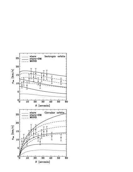
Figure 1: Upper panel: predicted line-of-sight velocity dispersion profiles for the Fornax dwarf in the case of isotropic orbits. The dotted line shows the prediction obtained by solving Jeans equation for stars only. The three solid lines correspond to stars + DM with the dark halo masses of $10^{8}$, $10^{9}$ and $10^{10}$ $M_{\sun}$ from bottom to top. The three dashed lines show results for stars in MOND with $a_{0}$ = 1, 3, 6 $\times 10^{-8}$ cm/s² from bottom to top. The data for Fornax are from Mateo (1997). Lower panel: same as upper panel, but for circular orbits.

Figure 1 shows the predicted line-of-sight velocity dispersion profiles for the Fornax dwarf together with the data from Mateo (1997). The two panels present results for different velocity anisotropy models. The upper panel gives the results in the case of isotropic orbits obtained from equations (3) and (5) in the limit of large $r_{\rm a}$. The lower panel is for circular orbits showing results from (6). The three types of curves in each panel correspond to the three possibilities of the velocity dispersion profile being generated 1) by stars moving under Newtonian gravitational acceleration generated by stars only (dotted curves), 2) by stars moving under Newtonian gravitational acceleration generated by stars and DM (solid lines), 3) by stars moving under modified (MONDian) acceleration generated by stars (dashed lines).

For all cases the 3D distribution of stars $\nu(r)$ is given by (9). The gravitational acceleration for the Newtonian cases 1) and 2) is $g=g_{\rm N}=-GM(r)/r^{2}$ with $M(r)=M_{*}(r)$ for 1) and $M(r)=M_{*}(r)+M_{\rm NFW}(r)$ for 2), where $M_{*}(r)$ and $M_{\rm NFW}(r)$ are given by equations (10) and (13), respectively. In the case of MOND we have $g=g_{\rm M}$ from equation (15) with $g_{\rm N}=-GM_{*}(r)/r^{2}$. The three solid curves in each panel correspond from bottom to top to the virial masses of the dark halo $M_{\rm v}=10^{8}$, $10^{9}$ and $10^{10}$ $M_{\sun}$. The three dashed lines show from bottom to top results obtained with different characteristic MOND acceleration scales $a_{0}$ = 1, 3, 6 $\times 10^{-8}$ cm/s².

Figure 2: Best-fitting models for Fornax based on stars+DM (solid line) and MOND (dashed line). The model involving DM has $\beta=-1.4$ and $M_{\rm v}=1.5\times 10^{9}M_{\sun}$. The model with MOND requires $\beta=-1$ and $a_{0}=2.1\times 10^{-8}$ cm/s².

Figure 1 clearly shows that the stars alone cannot reproduce the observed velocity dispersion profile of Fornax, unless the stellar mass-to-light ratio is much larger than assumed. In the following we will farther analyse the cases 2) and 3) trying to find the best-fitting models. Comparing the predictions shown in Figure 1 with the data we find that a certain amount of tangential anisotropy is needed to reproduce the shape of the observed velocity dispersion profile. Indeed, trying more radial anisotropy than in the case of isotropic orbits by using small values of $r_{\rm a}$ (comparable to $R_{\rm S}$ or $r_{\rm v}$) in (3) and (5) makes the curves in the upper panel of Figure 1 decrease even more steeply with distance, contrary to the trend observed in the data. Therefore in what follows we adopt the velocity anisotropy model of $\beta=$const$<0$ and treat $\beta$ as a free parameter.

To find the best models we performed a two-parameter fitting for each case. The fitting parameters were $(M_{\rm v},\beta)$ for stars+DM case and $(a_{0},\beta)$ for MOND. The results of minimizing $\chi^{2}$ weighted by the variances of the data points are shown in Figure 2. It turns out that the DM model fits the data best for $\beta=-1.4$ and $M_{\rm v}=1.5\times 10^{9}M_{\sun}$. This virial mass is more than two orders of magnitude larger than the stellar mass ($1.4\times 10^{7}M_{\sun}$ for $\Upsilon_{\rm V}=1M_{\sun}/L_{\sun}$). In the case of MOND the best-fitting parameters are $\beta=-1$ and $a_{0}=2.1\times 10^{-8}$ cm/s². This value of $a_{0}$ is consistent with other estimates (Milgrom 1983b).

Figure 3: The dependence of the mass-to-light ratio of Fornax on distance. The mass comes from stars and DM with the best fitting $M_{\rm v}=1.5\times 10^{9}M_{\sun}$.

Figure 3 shows the combined mass-to-light ratio in V-band for Fornax calculated from

$$M/L_{\rm V}=\frac{M_{\rm NFW}(r)+M_{*}(r)}{L_{\rm V}(r)},$$ (16)

where $M_{\rm NFW}(r)$ and $M_{*}(r)$ are given by equations (13) and (10) respectively, and $L_{\rm V}(r)=M_{*}(r)/\Upsilon_{\rm V}$ is the luminosity distribution. The shape of the curve reflects the fact that DM dominates both at small and large distances. The divergence of $M/L$ at the centre of the galaxy is due to the fact that the luminosity density (9) increases towards the centre more slowly than the DM cusp of $r^{-1}$ in (11). The growth of $M/L$ at large distances is due to the behaviour of $M_{\rm NFW}(r)$ which diverges logarithmically while the mass in stars is finite. The minimum of $M/L_{\rm V}\approx 11$ appears at a scale of the order of the Sérsic radius and is consistent with the values of the central mass-to-light ratio estimated by Mateo et al. (1991).

4 Discussion

We have found that the predictions based on MOND with $a_{0}=2.1\times 10^{-8}$ cm/s² fit the Fornax data equally well as models based on DM with virial mass of $M_{\rm v}=1.5\times 10^{9}M_{\sun}$. In both cases a certain amount of tangential anisotropy is needed to reproduce the shape of the observed velocity dispersion profile. It turned out that the MOND predictions in the case of Fornax dwarf need less tangential anisotropy than DM predictions to reproduce the shape of the velocity dispersion profile. It remains to be checked how the DM predictions depend on the particular shape of DM distribution.

The particular fitted values of $a_{0}$ and $M_{\rm v}$ are of course sensitive to the observational parameters assumed. The measured luminosity, distance and structural parameters of the dwarfs are all known with limited accuracy, but the detailed analysis of the errors in them is beyond the scope of this paper. In the case of MOND the most doubtful input parameter is the stellar mass-to-light ratio in V-band. We have assumed here $\Upsilon_{\rm V}\approx 1M_{\sun}/L_{\sun}$ characteristic for a relatively young stellar population of Fornax, however this value may well be different by a factor of two (Mateo et al. 1991). To estimate its effect we performed a similar MOND fitting as described in the previous section with $\Upsilon_{\rm V}=0.5$ and $2\ M_{\sun}/L_{\sun}$, obtaining respectively $a_{0}=4.3$ and $1.1\ \times 10^{-8}$ cm/s² with the same best-fitting $\beta$. If $\Upsilon_{\rm V}=0.5M_{\sun}/L_{\sun}$ is indeed the lower limit of mass-to-light ratio, then $a_{0}=4.3\times 10^{-8}$ cm/s² is the upper limit for $a_{0}$.

In the case of DM the stellar mass-to-light is not likely to influence much the results since the input from stars to the velocity dispersion is small. Here the most doubtful parameter is the concentration of DM haloes, which we adopted to follow the same dependence on mass as larger haloes actually studied in $N$-body simulations. Given, however, that this dependence is weak in the $\Lambda$CDM Universe, the possible error associated with this factor is rather small.

One more reason to worry are the tidal interactions that may affect the dynamics of some dwarfs and our interpretations of their velocity dispersions. Piatek & Pryor (1995) have performed numerical simulations of such effects and concluded that in Newtonian dynamics they should not affect much the inferred mass-to-light ratios (but see Kroupa 1997). However, Brada & Milgrom (2000) found that in MOND, due to its non-linearity, a galaxy system can be more affected by an external field.

Figure 4: Best-fitting models for Draco (left panel) and Ursa Minor (right panel) based on stars+DM (solid lines) and MOND (dashed lines). The data are from Armandroff et al. (1997)

One may ask if similar results hold for other dSph galaxies as well. Of those studied by IH the velocity dispersion profiles with a few data points are available only for Sextans, Ursa Minor and Draco dwarfs (Hargreaves et al. 1994a, 1994b, 1996; Armandroff, Olszewski & Pryor 1995; Armandroff, Pryor & Olszewski 1997). Applying the same analysis as we did for Fornax to the 5 data points for Draco and Ursa Minor from Armandroff et al. (1997) (with $\Upsilon_{\rm V}=1M_{\sun}/L_{\sun}$) we find that again the MOND and DM models can fit the data equally well. For Draco the best-fitting models have tangential anisotropy, we get $\beta=-0.9$, $M_{\rm v}=4.2\times 10^{9}M_{\sun}$ ($2\times 10^{4}$ the mass in stars) for DM and $\beta=-1.5$, $a_{0}=50\times 10^{-8}$ cm/s² for MOND. For Ursa Minor the best fits require a certain amount of radial anisotropy which we model with (2). We get $r_{\rm a}=0.014r_{\rm v}=0.86R_{\rm S}=0.16$ kpc, $M_{\rm v}=1.9\times 10^{8}M_{\sun}$ ($10^{3}$ the mass in stars) for DM and $r_{\rm a}=0.012r_{\rm v}=0.76R_{\rm S}=0.14$ kpc, $a_{0}=12\times 10^{-8}$ cm/s² for MOND. The predictions of the best-fitting models together with the data are shown in Figure 4.

The case of Ursa Minor is doubtful since it has been recently observed to possess tidal tails (Martínez-Delgado et al. 2001) and therefore may not be in virial equilibrium. The high value of $a_{0}$ estimated for Draco can, however, pose a serious problem for MOND (we agree on this point with Gerhard & Spergel 1992) since $a_{0}$ is supposed to be a universal constant. Bringing the value down by an order of magnitude would require very high stellar mass-to-light ratio $\Upsilon_{\rm V}\sim 10M_{\sun}/L_{\sun}$ or we would have to believe that the measurements seriously overestimate the velocity dispersion.

References

- [] Armandroff T. E., Olszewski E. W., Pryor C., 1995, AJ, 110, 2131
- [] Armandroff T. E., Pryor C., Olszewski E. W., 1997, in Sofue Y., ed., Proc. IAU Symp. 184, The Central Regions of the Galaxy and Galaxies. Kluwer, Dordrecht, p. 35
- [] Binney J., Mamon G. A., 1982, MNRAS, 200, 361
- [] Binney J., Tremaine S., 1987, Galactic Dynamics. Princeton Univ. Press, Princeton, chap. 4.4.3
- [] Brada R., Milgrom M., 2000, ApJ, 541, 556
- [] Caon N., Capaccioli M., D’Onofrio M., 1993, MNRAS, 265, 1013
- [] Caldwell N., 1999, AJ, 118, 1230
- [] Ciotti L., 1991, A&A, 249, 99
- [] Gerhard O., Kronawitter A., Saglia R. P., Bender R., 2001, AJ, 121, 1936
- [] Gerhard O. E., Spergel D. N., 1992, ApJ, 397, 38
- [] Hargreaves J. C., Gilmore G., Irwin M. J., Carter D., 1994a, MNRAS, 269, 957
- [] Hargreaves J. C., Gilmore G., Irwin M. J., Carter D., 1994b, MNRAS, 271, 693
- [] Hargreaves J. C., Gilmore G., Irwin M. J., Carter D., 1996, MNRAS, 282, 305
- [] Irwin M., Hatzidimitriou D., 1995, MNRAS, 277, 1354
- [] Jing Y. P., Suto Y., 2000, ApJ, 529, L69
- [] Kroupa P., 1997, NewA, 2, 139
- [] Lima Neto G. B., Gerbal D., Márquez I., 1999, MNRAS, 309, 481
- [] Łokas E. L., Mamon G. A., 2001, MNRAS, 321, 155
- [] Martínez-Delgado D, Alonso-García J., Aparicio A., Gómez-Flechoso M. A., 2001, ApJ, 549, L63
- [] Mateo M., 1997, in Arnaboldi M. et al., eds, ASP Conf. Ser. Vol. 116, The Nature of Elliptical Galaxies. Astron. Soc. Pac., San Francisco, p. 259
- [] Mateo M., 1998, in Richtler T., Braun J. M., eds, Proc. Bonn/Bochum-Graduiertenkolleg Workshop, The Magellanic Clouds and Other Dwarf Galaxies. Shaker Verlag, Aachen, p. 53
- [] Mateo M., Olszewski E. W., Welch D. L., Fischer P., Kunkel W., 1991, AJ, 102, 914
- [] Merritt D., 1985, AJ, 90, 1027
- [] Milgrom M., 1983a, ApJ, 270, 365
- [] Milgrom M., 1983b, ApJ, 270, 371
- [] Milgrom M., 1984, ApJ, 287, 571
- [] Milgrom M., 1995, ApJ, 455, 439
- [] Navarro J. F., Frenk C. S., White S. D. M., 1997, ApJ, 490, 493
- [] Osipkov L. P., 1979, PAZh, 5, 77
- [] Piatek S., Pryor C., 1995, AJ, 109, 1071
- [] Pryor C., Kormendy J., 1990, AJ, 100, 127
- [] Sérsic J. L., 1968, Atlas de Galaxies Australes, Observatorio Astronomico, Cordoba
- [] Thomas P. A. et al., 1998, MNRAS, 296, 1061