The mass of the white dwarf in the recurrent nova U Scorpii

Abstract

We present spectroscopy of the eclipsing recurrent nova U Sco. The radial velocity semi-amplitude of the primary star was found to be $K_{W}=93\pm 10$ km s^-1 from the motion of the wings of the HeII$\>\lambda 4686$Å  emission line. By detecting weak absorption features from the secondary star, we find its radial velocity semi-amplitude to be $K_{R}=170\pm 10$ km s^-1. From these parameters, we obtain a mass of $M_{1}=1.55\pm 0.24M_{\odot}$ for the white dwarf primary star and a mass of $M_{2}=0.88\pm 0.17M_{\odot}$ for the secondary star. The radius of the secondary is calculated to be $R_{2}=2.1\pm 0.2R_{\odot}$, confirming that it is evolved. The inclination of the system is calculated to be $i=82.7^{\circ}\pm 2.9^{\circ}$, consistent with the deep eclipse seen in the lightcurves. The helium emission lines are double-peaked, with the blue-shifted regions of the disc being eclipsed prior to the red-shifted regions, clearly indicating the presence of an accretion disc. The high mass of the white dwarf is consistent with the thermonuclear runaway model of recurrent nova outbursts, and confirms that U Sco is the best Type Ia supernova progenitor currently known. We predict that U Sco is likely to explode within $\sim 700\,000$ years.

1 Introduction

U Sco belongs to a small class of cataclysmic variables (CVs) known as recurrent novae (RNe), which show repeated nova outbursts on timescales of decades. Of these, U Sco has the shortest recurrence period ($\sim 8\>$y), with recorded outbursts in 1863, 1906, 1936, 1979, 1987 and 1999. It is likely that others have been missed due to its proximity to the ecliptic ($4^{\circ}$).

The RN class is further divided into three groups, depending on the nature of the secondary star (red giant, sub-giant or dwarf), each of which have different eruption mechanisms (see warner95a & webbink87 for reviews). U Sco is the only object of the three in the sub-giant class which eclipses (schaefer90), and also shows evidence of secondary absorption lines (hanes85), making it the best candidate for the determination of system parameters.

The outburst mechanism for the U Sco sub-class of RNe is believed to be a modified version of the thermonuclear runaway (TNR) model of classical novae outbursts (e.g. starrfield85). In this model, the primary star builds up a layer of material, accreted from the secondary star, on its surface. The temperature and density at the base of the layer become sufficiently high for nuclear reactions to begin. After ignition, the temperature rises rapidly and the reaction rates run away, until the radiation pressure becomes high enough to eject most of the accreted material. This process occurs when the accreted layer reaches a critical mass (truran86), the value of which is a strongly decreasing function of the white dwarf mass. Therefore, to reduce the time interval between eruptions to those observed in the RNe, either the mass accretion rate ($\dot{M}$) or the white dwarf mass must be increased. For RNe, the white dwarf mass is the more important constraint because there is an upper limit to $\dot{M}$ above which the degeneracy on the surface of the white dwarf weakens, and no powerful eruption can occur. For this model to account for the short times between outbursts as seen in RNe, the white dwarf must have a mass close to the Chandrasekhar limit. A tight constraint on the white dwarf mass in U Sco is hence theoretically important, as it will provide a direct observational test of the TNR model for this group of RNe.

The mass of the white dwarf in U Sco is also important in terms of binary evolution and the role of RNe as Type Ia supernova progenitors. livio94 suggested, on the basis of the abundance determinations of the ejecta of RNe, that the mass of the envelope ejected during the outburst might be smaller than the amount of accreted material. In the case of high mass white dwarf systems, the primary could be pushed over the Chandrasekhar limit to produce a supernova explosion. A tight constraint on the white dwarf mass and the mass accretion rate allows the time to supernova to be calculated, which according to starrfield88, could be as little as 50 000 years.

There have been two previous attempts to measure the mass of the white dwarf in U Sco. johnston92 attempted to use low resolution spectra to determine the radial velocity semi-amplitude of both components by looking at the emission and absorption line shifts. They calculated a white dwarf mass of 0.23–0.60$M_{\odot}$, a result disputed by Duerbeck93, who obtained 10 spectra with poor phase coverage, but were able to conclude a high primary mass, although their errors were large ($M_{1}=1.16\pm 0.69M_{\odot}$). schaefer95 re-phased the radial velocity measurements of johnston92 and Duerbeck93 using a new orbital period. They concluded that due to inconsistent $\gamma$ velocities, a phase shift in the emission lines and a large scatter in the radial velocity curves, no reliable white dwarf mass could be derived from the data.

In addition to this, hachisu00b sucessfully modelled the quiescent light curve of U Sco with a white dwarf mass of $M_{1}\sim 1.37M_{\odot}$, a secondary mass of $M_{2}=0.8$–$2.0M_{\odot}$ and an orbital inclination of $\sim 80^{\circ}$. Indirect support that the TNR model is the outburst mechanism in U Sco has also been found by the observation of luminous supersoft X-ray emission after the 1999 outburst (kahabka99). They also constrain the white dwarf to be massive from the temperature of the optically thick supersoft component.

In this paper, we present new measurements of the radial velocity semi-amplitude of the primary and secondary stars in U Sco and hence a new determination of the mass of the white dwarf in this system.

2 Observations

On the nights of 1999 April 15–19 we obtained 51 spectra of the recurrent nova U Sco with the 3.9m Anglo-Australian Telescope (AAT) in Siding Springs, Australia. We covered one complete orbit of U Sco during this time, including an eclipse – a full journal of observations is given in Table 1. The exposures were all 1500 s with about 50 s dead-time for archiving of data. The setup comprised of the RGO Spectrometer + 250mm camera, the TEK $1024\times 1024\;$ CCD chip and the 1200V grating, which gave a wavelength coverage of approximately 4620Å–5435Å  at 1.6Å  (95 km s^-1) resolution. We also took spectra of 20 class IV and V spectral type templates ranging from F0 – K2, and the flux standard LTT 9239 (hamuy92). The 1.5 arcsec slit was orientated to cover a comparison star $\sim 1$ arcmin west of U Sco in order to correct for slit losses. Arc spectra were taken between every U Sco exposure to calibrate instrumental flexure. The nights were all photometric, and the seeing varied between approximately 1.0 arcsec and 1.8 arcsec throughout the five nights.

Figure 1: R-band lightcurve of the 1999 outburst of U Sco. The data have been taken from matsumoto01. The open circle represents a measurement with an unrecorded error.

Table 1: Journal of observations for U Sco. Orbital phase is calculated using the new ephemeris presented in this paper (equation 1).

UT Date	UT		UT		No. of	Phase		Phase
	start		end		spectra	start		end
1999 April 15	14:	57	19:	09	8	0.	31	0.	44
1999 April 16	14:	14	19:	21	11	0.	09	0.	26
1999 April 17	14:	21	19:	11	10	0.	92	1.	07
1999 April 18	14:	20	19:	16	11	0.	72	0.	88
1999 April 19	14:	23	19:	30	11	0.	54	0.	70

U Sco underwent its sixth recorded outburst on 1999 February 25, reaching a maximum brightness of V = 7.6 (schmeer99). The observations recorded in this paper were taken approximately 49 days after outburst maximum, as can be seen from the lightcurve in Fig. 1, by which time the magnitude had decreased to approximately one magnitude above its quiescent level. Unfortunately, the single data point in Fig. 1 corresponding to the dates of our observations has no recorded uncertainty. It is therefore impossible to conclude whether we actually observed U Sco during an anomalously high state. What is certain, however, is that the additional shot noise in the continuum made it more difficult than we expected to detect absorption lines from the secondary star. The total flux in each spectrum is plotted in Fig. 2 as a function of Heliocentric Julian Date (HJD) following equation LABEL:eqn:ephem (see Section 4.1). The eclipse occurs on the third night of observation. There is also some evidence for a slight downward trend in brightness over the five nights.

3 Data Reduction

We debiased the data and corrected for the pixel-to-pixel variations with a tungsten lamp flat-field. The sky was subtracted by fitting second-order polynomials in the spatial direction to the sky regions on either side of the object spectra. The data were then optimally extracted (horne86a) to give raw spectra of U Sco and the comparison star. Arc spectra were then extracted from the same locations on the detector as the targets. The wavelength scale for each spectrum was interpolated from the wavelength scales of two neighbouring arc spectra. The root-mean-square error in the fourth-order polynomial fits to the arc lines was $\sim 0.025$Å.

The next stage of the reduction process was to correct for the instrumental response and slit losses in order to obtain absolute fluxes. A third-order spline fit to the continuum of the spectrophotometric standard star was used to remove the large-scale variations of instrumental response with wavelength. The slit-loss correction was performed by dividing the U Sco spectra by spline fits to the comparison star spectra, and then multipling the resulting spectra by a spline fit to a wide-slit comparison star spectrum.

4 Results

4.1 Ephemeris

The times of mid-eclipse were determined by fitting a parabola to the eclipse minimum (the solid curve in Fig. 2). A least-squares fit to the 9 eclipse timings found in schaefer95 and our eclipse yields the following ephemeris:

$$\begin{array}[]{lrrl}T_{\rm mid-eclipse}=&\!\!\!\!\!{\rm HJD}\,\,2\,447\,717.6145&\!\!+\,\,1.230\,5522&\!\!\!\!\!E\\ &\!\!\pm\,\,0.0044&\!\!\pm\,\,0.000\,0024&\\ \end{array}$$ (1)

The differences between the observed and calculated times of mid-eclipse are given in Table 2. We find no evidence for a non-zero value for $\dot{P}$, in agreement with schaefer95.

Table 2: Times of mid-eclipse for U Sco according to Schaefer & Ringwald (1995; SR95) and this paper.

Cycle	HJD at mid-eclipse		O-C		Reference
(E)	(2,440,000+)		(secs)
0	7717.5968$\>\pm\>$	0.0139	-1530.	6	SR95
1	7718.8412$\>\pm\>$	0.0069	-334.	1	SR95
4	7722.5318$\>\pm\>$	0.0139	-425.	4	SR95
5	7723.7783$\>\pm\>$	0.0139	952.	5	SR95
8	7727.4699$\>\pm\>$	0.0139	947.	6	SR95
1168	9154.9111$\>\pm\>$	0.0104	1003.	5	SR95
1496	9558.5240$\>\pm\>$	0.0069	293.	1	SR95
1497	9559.7497$\>\pm\>$	0.0069	-126.	1	SR95
1500	9563.4432$\>\pm\>$	0.0139	33.	2	SR95
2900	11286.2143$\>\pm\>$	0.0050	-141.	3	This Paper

Figure 2: Light curve of U Sco during our observations. The solid curve is a parabolic fit to the eclipse minimum.

4.2 Average Spectrum

The average spectrum of U Sco is displayed in Fig. 3, and in Table 3 we list fluxes, equivalent widths and velocity widths of the most prominent lines measured from the average spectrum.

The spectrum is dominated by single-peaked emission lines between $\lambda\lambda$4870–5080Å  originating from the recent outburst. The identification of these nebular lines is complicated by their large widths, but the blend is likely to have contributions from NII, NIII, NV, OIII and OV, indicating a very high degree of excitation. Both sekiguchi88 and munari99 attribute the complex around $\lambda$5015Å  to a blend of He I and NII in the 1987 and 1999 outbursts, respectively. barlow81 suggest in the 1979 outburst the presence of H$\beta$ at $\lambda 4861$Å, and strong OIII emission at $\lambda\lambda$4959/5007Å. This is supported by comparison with nebulae around classical novae such as Nova Cygni 1992 (moro01). There is also evidence of CIV emission at $\lambda 4658$Å, in agreement with the 1987 outburst (sekiguchi88). The other strong features in the blend are likely to be due to NIII and NV, in agreement with barlow81, and optical spectra of Nova GQ Muscae 1983 (pequignot93). It is difficult to directly compare our spectra to the spectra of the 1979 outburst (barlow81) and the 1987 outburst (sekiguchi88) because the latter two datasets were taken much closer to the eruption.

U Sco also shows strong, broad, double-peaked He II lines at $\lambda$4686Å  and $\lambda$5412Å, typical of emission from an accretion disc in a high inclination system (e.g. horne86).

The secondary star features cannot clearly be seen in Fig. 3, as the spectra have been averaged without being corrected for orbital motion. Consequently, any faint absorption lines will have been smeared out.

However, when the orbital motion of the secondary star is removed, the MgIb triplet ($\lambda\lambda$5167,5173,5184Å) can clearly be identified (see Section 4.7 and Figure 10).

Figure 3: The average spectrum of U Sco, uncorrected for orbital motion.

Table 3: Fluxes and widths of prominent lines in U Sco, measured from the average spectrum. The wavelength range of the blend is $\lambda\lambda$4870–5080Å.

Line		Flux			EW			FWHM			FWZI
		$\times$ 10-14			Å			km s-1			km s-1
		ergs cm-2 s-1
HeII$\>\lambda$4686Å		1.345$\>\pm\>$	0.007		6.98$\>\pm\>$	0.04		700$\>\pm\>$	50		1600$\>\pm\>$	100
HeII$\>\lambda$5412Å		0.177$\>\pm\>$	0.005		1.18$\>\pm\>$	0.03		700$\>\pm\>$	100		1500$\>\pm\>$	300
Blend		11.95$\>\pm\>$	0.02		82.9$\>\pm\>$	0.1

4.3 Light Curves

The continuum light curve for U Sco was computed by summing the flux in the wavelength range $\lambda\lambda$5080–5390Å, which is devoid of emission lines. A polynomial fit to the continuum was then subtracted from the spectra and the emission line light curves were computed by summing the residual flux after continuum subtraction.

The resulting light curves are plotted in Fig. 4 as a function of phase, following our new ephemeris. The continuum shows a symmetrical eclipse, with flickering throughout. There appears to be a dip in magnitude around phase 0.5, perhaps indicative of a secondary eclipse, but there are too few data points to be conclusive. In addition, as a consequence of U Sco’s long orbital period (1.23 days), the lightcurves represent data from five nights. Therefore, not all of the variability can be necessarily attributed to orbital effects.

The eclipses of the HeII lines have a different shape from the continuum. Both lightcurves show a long egress, and a pre-eclipse increase in brightness. There is no evidence for significant variability in the lightcurve of the nebular lines ($\lambda\lambda$4870–5080Å), supporting the idea that the lines are produced in a region external to the orbits of the stellar components.

Figure 4: Continuum and emission line lightcurves of U Sco. The open circles represent points where the real data (the closed circles) have been folded over.

4.4 Trailed spectrum

We subtracted polynomial fits to the continua from the spectra and then rebinned the spectra onto a constant velocity-interval scale centred on the rest wavelength of the lines. The rest wavelength of the nebular lines was taken as $\lambda 4975$Å. The data were then phase binned into 40 bins, 36 of which were filled. Fig. 5 shows the trailed spectra of the HeII $\lambda 4686$Å, HeII $\lambda 5412$Å  and nebular lines in U Sco.

The HeII lines show two peaks, which vary sinusoidally with phase. This, and the rotational disturbance (where the blue-shifted peak is eclipsed before the red-shifted peak) is evidence for origin in a high inclination accretion disc. There is also some evidence for an emission component moving from blue to red between phases 0.6 – 0.9.

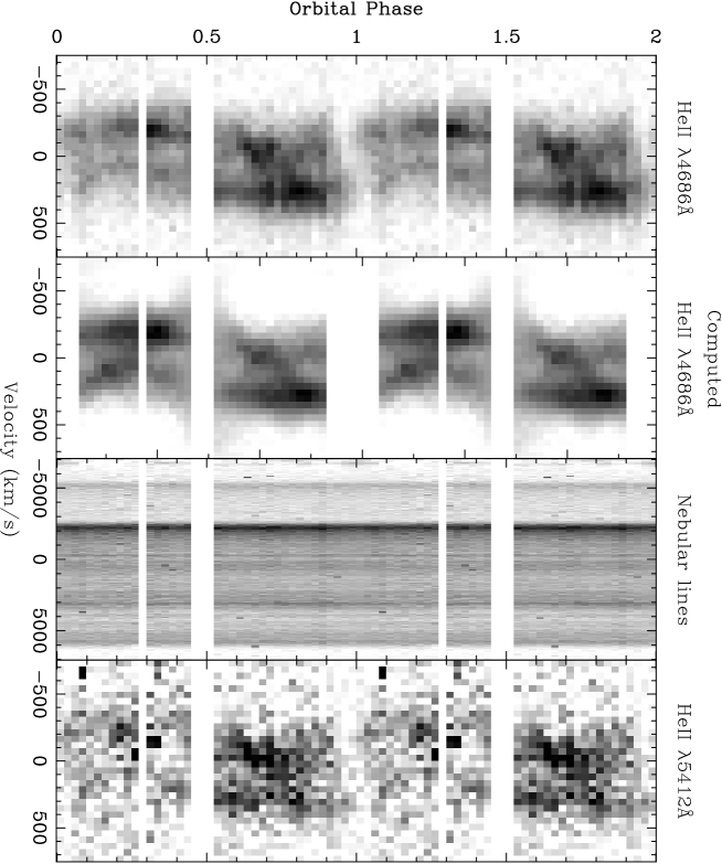
Figure 5: Trailed spectra of HeII $\lambda 4686$ Å, the nebular lines and HeII $\lambda 5412$ Å. The second panel from the left shows the HeII $\lambda 4686$ Å  line computed from the Doppler map. The gaps around phases 0 and 1 in the computed data correspond to eclipse data, which were omitted from the fit; the gaps around phases 0.3, 0.5, 1.3 and 1.5 are due to missing data. The data only cover one cycle, but are folded over for clarity.

4.5 Doppler Tomography

Doppler tomography is an indirect imaging technique which can be used to determine the velocity-space distribution of line emission in cataclysmic variables. For a detailed review of Doppler tomography, see marsh00.

Fig. 6 shows the Doppler map of the HeII$\;\lambda 4686$Å  line in U Sco, computed from the trailed spectra of Fig. 5 but with the eclipse spectra removed. The data for the HeII$\>\lambda 5412$Å  line were too noisy to produce a Doppler map. The three crosses on the Doppler map represent the centre of mass of the secondary star (upper cross), the centre of mass of the system (middle cross) and the centre of mass of the white dwarf (lower cross). These crosses, the Roche lobe of the secondary star, and the predicted trajectory of the gas stream have been plotted using the radial velocities of the primary and secondary stars, $K_{W}=93\pm 10$ km s^-1 and $K_{R}=170\pm 10$ km s^-1, derived in Section 4.9. The series of circles along the gas stream mark the distance from the white dwarf at intervals of $0.1L_{1}$, ranging from $1.0L_{1}$ at the red star to $0.3L_{1}$.

A ring-like emission distribution, characteristic of a Keplerian accretion disc centred on the white dwarf, is clearly seen in Fig. 6. There is some evidence for an increase in emission downstream from where the computed gas stream joins the accretion disc, implying the presence of a bright spot. This kind of behaviour has been seen in other CVs – e.g. WZ Sge (spruit98).

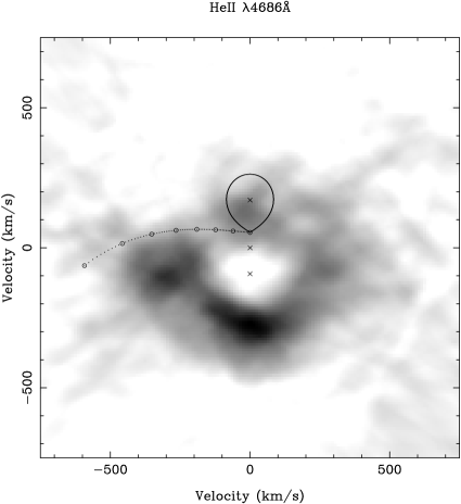
Figure 6: Doppler map of HeII$\>\lambda 4686$Å  emission in U Sco.

4.6 Radial velocity of the white dwarf

The continuum-subtracted data were binned onto a constant velocity interval scale about each of the two helium line rest wavelengths. In order to measure the velocities, we used the double-Gaussian method of schneider80, since this technique is sensitive mainly to the motion of the line wings and should therefore reflect the motion of the white dwarf with the highest reliability. We varied the Gaussian widths between 150–300 km s^-1 at 50 km s^-1 intervals, as well as varying their separation $a$ from 200–1500 km s^-1. We then fitted

$$V=\gamma-K\sin[2\pi(\phi-\phi_{0})]$$ (2)

to each set of measurements, omitting the 9 points around primary eclipse which were affected by the rotational disturbance. An example of a radial velocity curve obtained for the HeII $\lambda 4686$Å  line for a Gaussian width of 300 km s^-1 and separation 1000 km s^-1 is shown in Fig. 7. The data for the HeII $\lambda 5412$Å  line were too noisy to determine accurate radial velocities.

Figure 7: Radial velocity curve of HeII $\lambda 4686$Å, measured using a double-Gaussian fit with a separation of 1000 km s^-1. Points marked by open circles were not included in the radial velocity fit, as they were affected by the rotational disturbance during primary eclipse. The horizontal dashed line represents the systemic velocity.

The radial velocity curve has a negligible phase offset, an indication that the helium line is a reliable representation of the motion of the white dwarf. The results of the radial velocity analysis are displayed in the form of a diagnostic diagram in Fig. 8. By plotting $K$, its associated fractional error $\sigma_{K}/K$, $\gamma$ and $\phi_{0}$ as functions of the Gaussian separation, it is possible to select the value of $K$ that most closely represents the actual $K_{W}$ (shafter86). If the emission were disc dominated, one would expect the solution for $K$ to asymptotically reach $K_{W}$ when the Gaussian separation becomes sufficiently large, and furthermore, one would expect $\phi_{0}$ to fall to 0. This is seen to occur at a separation of $\sim$1200 km s^-1, corresponding to $K_{W}\sim\>$93 km s^-1. There is, however, no sudden increase in $\sigma_{K}/K$, prompting us to employ a different approach.

Figure 8: The diagnostic diagram for U Sco based on the double-Gaussian radial velocity fits to HeII $\lambda 4686$Å.

marsh88a suggests that the use of a diagnostic diagram to evaluate $K_{W}$ does not account for systematic distortion of the radial velocity curve. We therefore attempted to make use of the light centres method, as described by marsh88a. In the co-rotating co-ordinate system, the white dwarf has velocity ($0,-K_{W}$), and symmetric emission, say from a disc, would be centred at that point. By plotting $K_{x}=-K\sin\phi_{0}$ versus $K_{y}=-K\cos\phi_{0}$ for the different radial velocity fits (Fig. 9), one finds that the points move closer to the $K_{y}$ axis with increasing Gaussian separation. A simple distortion which only affects low velocities, such as a bright spot, would result in this pattern, equivalent to a decrease in distortion as one measures emission closer to the velocity of the primary star. By extrapolating the last point on the light centre diagram to the $K_{y}$ axis, we measure the radial velocity semi-amplitude of the white dwarf $K_{W}=93\pm 10$ km s^-1. The error on $K_{W}$ was estimated from the uncertainty in crossing the $K_{y}$ axis, given the uncertainties associated with the points on the light centres diagram. Note the small scale on the $x$–axis of the light centres diagram.

Figure 9: Light centres diagram for HeII$\>\lambda 4686$Å  in U Sco.

4.7 Radial velocity of the secondary star

The secondary star in U Sco is observable through weak absorption lines, although many features have been drowned out by the nebular lines of the outburst. We compared regions of the spectra rich in absorption lines with several template dwarfs of spectral types F0–K2, the spectra of which are plotted in Fig. 10. The absorption features are too weak for the normal technique of cross-correlation to be successful in finding the value of $K_{R}$, but it is possible to exploit these features to obtain an estimate of $K_{R}$ using the technique of skew mapping. This technique is descibed by smith93b.

The first step was to shift the spectral type template stars to correct for their radial velocities. We then normalized each spectrum by dividing by a spline fit to the continuum and then subtracting 1 to set the continuum to zero. This ensures that line strength is preserved along the spectrum. The U Sco spectra were also normalized in the same way. The template spectra were artificially broadened by 16 km s^-1 to account for orbital smearing of the U Sco spectra through the 1500 s exposures. The rotational velocity of the secondary star was found by the equation

$$q(1+q)^{2}=9.6\Biggl{(}{{v\sin i}\over{K_{R}}}\Biggr{)}^{3}$$ (3)

(smith98) using estimated values of $q$ and $K_{R}$ in the first instance, then iterating to find the best fit values given in Section 4.9. The templates were then broadened by this value of $v\sin i$ = 88 km s^-1. Regions of the spectrum devoid of emission lines ($\lambda\lambda 5085-5395$Å) were then cross-correlated with each of the templates yielding a time series of cross-correlation functions (CCFs) for each template star.

Figure 10: Normalized spectra of ten template stars. The offset between each is 0.035. The U Sco spectrum is a normalized average of 43 of the 51 spectra observed; 8 spectra were omitted due to cosmic rays interfering with secondary features. The template spectra have been broadened by 16 km s^-1 to account for orbital smearing of the U Sco spectra during exposure and by 88 km s^-1 to account for the rotational broadening of the lines in U Sco.

To produce the skew map (Fig. 11), these CCFs were back-projected in the same way as time-resolved spectra in standard Doppler tomography (marsh88b). If there is a detectable secondary star, we would expect a peak at (0,$K_{R}$) in the skew map. This can be repeated for each of the templates.

When we first back-projected the CCFs, the peak in each skew map was seen to be displaced to the blue of the $K_{x}=0$ axis by around 30 km s^-1. The reason was that we assumed that the centre of mass of the system was at rest. The systemic velocity of U Sco derived from the radial velocity curve fits in Section 4.6 is $\gamma=47\pm 10\>$km s^-1. Applying this $\gamma$ velocity shifts the peak to the red, towards the $K_{x}=0$ axis. As $K_{x}^{2}\ll K_{y}^{2}$, then the value of $K_{R}$ is given by the equation

$$K_{R}=(K_{x}^{2}+K_{y}^{2})^{1/2}\approx K_{y},$$

so $K_{R}$ changes little whilst varying $\gamma$.

The skew maps produced using each of the template stars with $\gamma=0\>$km s^-1 show well-defined peaks at $(K_{x},K_{y})\sim(-30,160)\>$km s^-1. However, applying $\gamma=47\>$km s^-1, the peaks in the skew maps shift to $(K_{x},K_{y})\sim(15,180)\>$km s^-1. We suspect that the true $\gamma$ value of U Sco falls between these two limits. The skew map shown in Fig. 11 is for the K2V spectral type template with $\gamma$ = 47 km s^-1, and is arguably the best fitting template for the secondary star. The skew map shows a clear peak around $(K_{x},K_{y})\sim(10,165)\>$km s^-1. To bring the skew map peak to lie on $K_{x}=0$, the $\gamma$ value must be modified to $\sim$ 30 km s^-1, which still falls within $2\sigma$ of the $\gamma$ derived from the emission lines. The resulting peak falls on $K_{y}=170$ km s^-1, which we adopt as the radial velocity semi-amplitude for the secondary star: $K_{R}=170\pm 10$ km s^-1. The uncertainty in $K_{R}$ has been determined from the scatter in $K_{R}$ due to four sources of error: varying the $\gamma$ velocity; using different spectral type templates; producing skew maps from random subsets of the data; the accuracy in measuring the peak in the skew map.

The bottom panel of Fig. 11 shows a sine wave in the trailed CCFs, demonstrating that the peak in the skew map is not due to noise in the CCFs. It can be seen that the peaks in the CCFs are most prominent around primary eclipse ($\phi\sim$ 0.7–1.2). There are two possible explanations for this. First, by considering the geometry of the secondary eclipse in U Sco, we estimate that a maximum of 30 per cent of the visible surface of U Sco will be obscured by the large accretion disc (see Section 4.9) between phases 0.35–0.65. We would therefore expect the peaks in the CCFs to weaken considerably at these phases, which is exactly as observed in Figure 11. This explanation is further supported by the tentative evidence for a secondary eclipse presented in the continuum light curve (Figure 4) and it does not affect the values for the masses we have derived in Section 4.9. Second, it is possible that the absorption features on the inner hemisphere of the secondary star are weakened by irradiation due to the recent outburst, which would again explain the loss of the peaks in the CCFs around phase 0.5. If the latter explanation were true, it is possible that we have overestimated the value of $K_{R}$, which would in turn lead us to overestimate $M_{1}$ (see Figure 12). The only way we can reliably account for any systematic effects due to irradiation would be to obtain higher signal-to-noise observations during quiescence and so measure $v\sin i$ during primary eclipse.

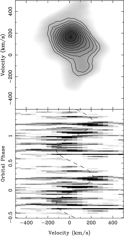
Figure 11: The top panel shows the skew map of U Sco for the K2V spectral type template. The bottom panel shows the trailed CCFs for the same template, clearly demonstrating that the peak in the skew map represents $K_{R}$ and is not an artefact of noise in the CCFs. The dashed line shows our adopted parameters for the secondary star orbit: $K_{R}=170$ km s^-1, $\gamma=47$ km s^-1 and zero phase shift. The data have been folded over for clarity.

4.8 Rotational velocity and spectral type of the secondary star

Mass estimates of CVs using emission line studies suffer from systematic errors, and have been thoroughly discussed by a number of authors (e.g. marsh88a). More reliable mass estimates can be obtained by using $K_{R}$ in conjunction with the rotational velocity of the secondary star, $v\sin i$. We attempted to determine $v\sin i$ using the procedure outlined in sad98b, but the data were too noisy.

Previous estimates of the secondary spectral type have ranged from F5V to K2III. hanes85 suggests G0$\pm$5III-V, corroborated by webbink87 with a GIII subgiant. Recent estimates have agreed on the subgiant nature of the secondary. schaefer90 estimated the spectral type as G3-6 from the colours at minimum light, whereas johnston92 measured the observed ratio of calcium lines to H$\delta$ and found F8$\pm$2. Based on the detection of the MgI$b$ absorption in the 1979 outburst spectrum, kahabka99 find the secondary to be consistent with a low-mass subgiant secondary of spectral type K2. This is supported by anupama00, who estimate the secondary to be a K2 subgiant based on the indices of the MgI$b$ absorption band and the FeI + CaI absorption feature in the late-decline spectrum of the 1999 outburst. Unfortunately, as can be seen in Fig. 10, it is impossible to confirm a secondary spectral type using our data, although the MgI$b$ complex is clearly present.

4.9 System Parameters

The radial velocity curves show little or no phase shift, giving us confidence that our measurement of $K_{W}$ reflects the motion of the white dwarf. Hence, together with $K_{R}$, our newly derived period and a measurement of the eclipse full width at half-depth ($\Delta\phi_{1/2}$), we can proceed to calculate accurate masses free of many of the assumptions which commonly plague CV mass determinations. Our white dwarf radial velocity semi-amplitude, $K_{W}=93\pm 10$ km s^-1 compares favourably with the previous measurement of $K_{W}=95\pm 50$ km s^-1 by barlow81 after the 1979 outburst. schaefer95 derived the values $K_{W}=87\pm 32$ km s^-1 and $K_{R}=56\pm 27$ km s^-1, but concluded that these results were unreliable due to inconsistent $\gamma$ velocities, a phase shift in the emission lines and a large scatter in the radial velocity curves.

In order to determine $\Delta\phi_{1/2}$, we estimated the levels of flux outside the eclipse (the principle source of the error) and at eclipse minimum, and then measured the full width of eclipse half way between these points. The eclipse full width at half-depth for U Sco was measured to be $\Delta\phi_{1/2}=0.104\pm 0.01$, in good agreement with $\Delta\phi_{1/2}=0.106\pm 0.01$ cited by schaefer95.

We have opted for a Monte Carlo approach similar to that of horne93 to calculate the system parameters and their errors. For a given set of $K_{W}$, $K_{R}$, $\Delta\phi_{1/2}$ and $P$, other system parameters are calculated as follows.

Figure 12: Constraints on the masses of the stars in U Sco. Each dot represents an ($M_{1},M_{2}$) pair. The dashed lines are lines of constant inclination ($i=80^{\circ}$, $i=85^{\circ}$, $i=90^{\circ}$). The solid curves satisfy the constraints on $K_{W}=93\pm 10$ km s^-1 and $K_{R}=170\pm 10$ km s^-1.

The mass ratio, $q$, can be determined from the ratio of the radial velocities

$${q}={M_{1}\over M_{2}}={K_{W}\over K_{R}}.$$ (4)

$R_{2}/a$ can be estimated because we know that the secondary star fills its Roche lobe (as there is an accretion disc present and hence mass transfer). $R_{2}$ is the equatorial radius of the secondary star and $a$ is the binary separation. We used Eggleton’s formula (eggleton83) which gives the volume-equivalent radius of the Roche lobe to better than 1 per cent, which is close to the equatorial radius of the secondary star as seen during eclipse,

$${{R_{2}}\over a}={{0.49q^{2/3}}\over{{0.6q^{2/3}+\ln{(1+q^{1/3})}}}}.$$ (5)

By considering the geometry of a point eclipse by a spherical body (e.g. dhillon91), the radius of the secondary can be shown to be

$$\biggl{(}{{R_{2}}\over a}\biggr{)}^{2}=\sin^{2}\pi\Delta\phi_{1/2}+\cos^{2}\pi\Delta\phi_{1/2}\cos^{2}i.$$ (6)

Using the value of $R_{2}/a$ obtained from equation 5, combined with equation 6, the inclination of the system can be found. Kepler’s Third Law gives

$${{K_{R}^{3}P_{orb}}\over{2\pi G}}={{M_{1}\sin^{3}i}\over{(1+q)}^{2}}$$ (7)

which, with the values of $q$ and $i$ calculated using equations 4, 5 & 6, gives the mass of the primary star. The mass of the secondary star can then be obtained using equation 4. The distance of each component to the centre of mass of the system ($a_{1}$,$a_{2}$), is given by

$${a_{(1,2)}={{K_{(W,R)}P}\over{2\pi\sin{i}}}}$$ (8)

The separation of the two components, $a$, is $a_{1}+a_{2}$, allowing the radius of the secondary star, $R_{2}$, to be calculated from equation 5.

The Monte Carlo simulation takes 10 000 values of $K_{W}$, $K_{R}$, and $\Delta\phi_{1/2}$ (the error on the period is deemed to be negligible in comparison to the errors on $K_{W}$, $K_{R}$, and $\Delta\phi_{1/2}$), treating each as being normally distributed about their measured values with standard deviations equal to the errors on the measurements. We then calculate the masses of the components, the inclination of the system, the radius of the secondary star, and the separation of the components, as outlined above, omitting ($K_{W}$,$K_{R}$,$\Delta\phi_{1/2}$) triplets which are inconsistent with $\sin i\leq 1$. Each accepted $M_{1},M_{2}$ pair is then plotted as a point in Fig. 12, and the masses and their errors are computed from the mean and standard deviation of the distribution of spots. The solid curves in Fig. 12 satisfy the white dwarf radial velocity constraint, $K_{W}=93\pm 10$ km s^-1 and the secondary star radial velocity constraint, $K_{R}=170\pm 10$ km s^-1. We find that $M_{1}=1.55\pm 0.24M_{\odot}$ and $M_{2}=0.88\pm 0.17M_{\odot}$. The inclination of the system is calculated to be $i=82.7^{\circ}\pm 2.9^{\circ}$, consistent with the nature of the deep eclipse seen in the lightcurves and the presence of double-peaked helium emission.

Table 4: System parameters for U Sco

Parameter	Measured Value		Monte Carlo Value
$P_{orb}$ (d)	1.2305522
$K_{W}$ (km s-1)	93$\>\pm\>$	10	95$\>\pm\>$	9
$K_{R}$ (km s-1)	170$\>\pm\>$	10	169$\>\pm\>$	10
$\Delta\phi_{1/2}$	0.104$\>\pm\>$	0.010	0.098$\>\pm\>$	0.007
$q$			0.55$\>\pm\>$	0.07
$i^{\circ}$			82.7$\>\pm\>$	2.9
$M_{1}/M_{\odot}$			1.55$\>\pm\>$	0.24
$M_{2}/M_{\odot}$			0.88$\>\pm\>$	0.17
$R_{2}/R_{\odot}$			2.1$\>\pm\>$	0.2
$a/R_{\odot}$			6.5$\>\pm\>$	0.4
$\Delta\phi$	0.12$\>\pm\>$	0.01
$R_{D}/R_{1}$	0.87$\>\pm\>$	0.11

We computed the radius of the accretion disc in U Sco using the geometric method outlined in dhillon91. The phase half-width of eclipse at maximum intensity was found to be $\Delta\phi=0.12\pm 0.01$ from Figure 4. Combining $\Delta\phi$ with $q$ and $i$ derived above produces an accretion disc radius of $R_{D}=0.87\pm 0.11R_{1}$, where $R_{1}$ is the volume radius of the primary’s Roche lobe. Our values for $\Delta\phi$ and $R_{D}$ are consistent with those found by harrop96: $\Delta\phi=0.129\pm 0.008$ and $R_{D}\geq 0.92R_{1}$.

The empirical relation obtained by smith98 between mass and radius for the secondary stars in CVs is given by,

$${R\over R_{\odot}}=(0.93\pm 0.09)\Biggl{(}{M\over M_{\odot}}\Biggr{)}+(0.06\pm 0.03).$$ (9)

This predicts that if the secondary star is on the main-sequence, it should have a radius of 0.88$R_{\odot}$. The value we find is $2.1\pm 0.2R_{\odot}$, clearly indicating that the white dwarf in U Sco has an evolved companion.

The values of all the system parameters of U Sco derived in this section are listed in Table 4.

5 Discussion

5.1 TNR Model

The outburst events in RNe could be the result of the TNR model, as seen in classical novae, or the disc instability model of dwarf novae. It is likely that given the heterogeneous nature of RNe, the mechanism depends on the individual system (webbink90). In the case of U Sco, the TNR model was suggested in the light of severe problems with the disc instability model (webbink87). The motivation behind measuring the mass of the white dwarf in U Sco was to give positive confirmation that outbursts are the result of a TNR, which predicts that the higher the mass of the white dwarf, the more frequent the outbursts. For eruptions to recur on the timescales seen in U Sco ($\sim$ 8 years), the mass of the white dwarf must be very close to the Chandrasekhar mass of $1.378M_{\odot}$ (starrfield85; starrfield88; nomoto84). Our observations allow us to calculate the mass of the white dwarf in U Sco to be $M_{1}=1.55\pm 0.24M_{\odot}$. Despite the large error on the value, we can conclude that U Sco contains a high mass white dwarf, although additional work, such as an accurate $v\sin i$ determination during quiescence, must be done to further constrain this.

5.2 U Sco as a Type Ia SN Progenitor

Type Ia supernovae (SNe Ia) are widely believed to be thermonuclear explosions of mass-accreting white dwarfs (see nomoto97 for a review). The favoured model for progenitor binary systems is the Chandrasekhar mass model, in which a mass-accreting carbon-oxygen white dwarf grows in mass up to the Chandrasekar limit and then explodes as a SN Ia. For the evolution of accreting WDs towards the Chandrasekhar mass, two scenarios have been proposed. The first is a double degenerate scenario, where two white dwarfs merge to cross the Chandrasekhar limit. A candidate for this has been identified in KPD 1930+2752 (maxted01). The second is a single degenerate scenario, where matter is accreted via mass transfer from a stellar companion. A new evolutionary path for single degenerate progenitor systems is discussed by hachisu99, which descibes how the secondary (a slightly evolved main-sequence star) becomes helium rich. Their progenitor model predicts helium enriched matter accretion onto a white dwarf. Objects which display these characteristics in the form of strong HeII$\>\lambda 4686$Å  lines are luminous super-soft X-ray sources and certain recurrent novae, such as U Sco and the others in the U Sco subclass (V394 CrA and LMC-RN). The observations in this paper, in confirming the helium rich accreted matter, and constraining the white dwarf mass to be near the Chandrasekhar mass, make U Sco the best candidate for this evolutionary path to a SN Ia.

The time to supernova can be estimated by dividing the amount of mass required to reach the Chandrasekhar mass by the average mass accretion rate ($\dot{M}_{av}$). Our results suggest a minimum white dwarf mass of $\sim 1.31M_{\odot}$, which requires it to accrete approximately 0.07$M_{\odot}$ to become a SN Ia. In their model, hachisu00a find that the white dwarf in U Sco grows in mass at an average rate of $\dot{M}_{av}\sim 1.0\times 10^{-7}M_{\odot}$ y^-1. Using this value, we therefore predict U Sco to become a supernova within $\sim 700\,000$ years.

6 Conclusions

1. We have shown that U Sco contains a high mass white dwarf ($M_{1}=1.55\pm 0.24M_{\odot}$), confirming that the outburst mechanism is the TNR model.

2. The presence of an accretion disc has been confirmed for the first time by clear evidence of rotational disturbance in the HeII emission lines during eclipse, as well as their double-peaked nature.

3. The secondary star has a radius of $2.1\pm 0.2R_{\odot}$, consistent with the idea that it is evolved.

4. The mass of the white dwarf in U Sco is $M_{1}=1.55\pm 0.24M_{\odot}$, implying that it is the best SN Ia candidate known and is expected to explode in $\sim$ 700 000 years.

References

- [\citefmtAnupama & Dewangan2000] Anupama G. C., Dewangan G. C., 2000, AJ, 119, 1359
- [\citefmtBarlow et al.1981] Barlow M. J. et al., 1981, MNRAS, 195, 61
- [\citefmtDhillon, Marsh & Jones1991] Dhillon V. S., Marsh T. R., Jones D. H. P., 1991, MNRAS, 252, 342
- [\citefmtDuerbeck et al.1993] Duerbeck et al., 1993, ESO Messenger, 71, 19
- [\citefmtEggleton1983] Eggleton P. P., 1983, ApJ, 268, 368
- [\citefmtHachisu et al.1999] Hachisu I., Kato M., Nomoto K., Umeda H., 1999, ApJ, 519, 314
- [\citefmtHachisu et al.2000a] Hachisu I., Kato M., Kato T., Matsumoto K., Nomoto K., 2000a, ApJ, 534, L189
- [\citefmtHachisu et al.2000b] Hachisu I., Kato M., Kato T., Matsumoto K., 2000b, ApJ, 528, L97
- [\citefmtHamuy et al.1992] Hamuy M., Walker A. R., Suntzeff N. B., Gigoux P., Heathcote S. R., Phillips M. M., 1992, PASP, 104, 677
- [\citefmtHanes1985] Hanes D. A., 1985, MNRAS, 213, 443
- [\citefmtHarrop-Allin & Warner1996] Harrop-Allin M. K., Warner B., 1996, MNRAS, 279, 219
- [\citefmtHorne & Marsh1986] Horne K., Marsh T. R., 1986, MNRAS, 218, 761
- [\citefmtHorne, Welsh & Wade1993] Horne K., Welsh W. F., Wade R. A., 1993, ApJ, 410, 357
- [\citefmtHorne1986] Horne K., 1986, PASP, 98, 609
- [\citefmtJohnston & Kulkarni1992] Johnston H. M., Kulkarni S. R., 1992, ApJ, 396, 267
- [\citefmtKahabka et al.1999] Kahabka P., Hartmann H. W., Parmar A. N., Negueruela I., 1999, AA, 347, L43
- [\citefmtLivio & Truran1994] Livio M., Truran J. W., 1994, ApJ, 425, 797
- [\citefmtMarsh & Horne1988] Marsh T. R., Horne K., 1988, MNRAS, 235, 269
- [\citefmtMarsh1988] Marsh T. R., 1988, MNRAS, 231, 1117
- [\citefmtMarsh2000] Marsh T. R., 2000, in Boffin H., Steeghs D., eds, Proceedings of the International Workshop on Astro-tomography, Brussels, July 2000. Springer-Verlag Lecture Notes in Physics, in press
- [\citefmtMatsumoto, Kato & Hachisu2001] Matsumoto K., Kato K., Hachisu I., 2001, PASP, submitted
- [\citefmtMaxted, Marsh & North2000] Maxted P. F. L., Marsh T. R., North R. C., 2000, MNRAS, 317, L41
- [\citefmtMoro-Martín, Garnavich & Noriega-Crespo2001] Moro-Martín A., Garnavich P. M., Noriega-Crespo A., 2001, AJ, 121, 1636
- [\citefmtMunari et al.1999] Munari U. et al., 1999, AA, 347, L39
- [\citefmtNomoto, Iwamoto & Kishimoto1997] Nomoto K., Iwamoto K., Kishimoto N., 1997, Sci, 276, 1378
- [\citefmtNomoto, Thielemann & Yokoi1984] Nomoto K., Thielemann F., Yokoi K., 1984, ApJ, 286, 644
- [\citefmtPéquignot et al.1993] Péquignot D., Petitjean P., Boisson C., Krautter J., 1993, AA, 271, 219
- [\citefmtSchaefer & Ringwald1995] Schaefer B. E., Ringwald F. A., 1995, ApJ, 447, L45
- [\citefmtSchaefer1990] Schaefer B. E., 1990, ApJ, 355, L39
- [\citefmtSchmeer et al.1999] Schmeer P., Waagen E., Shaw L., Mattiazzo M., 1999, IAU Circ., 7113, 1
- [\citefmtSchneider & Young1980] Schneider D. P., Young P. J., 1980, ApJ, 238, 946
- [\citefmtSekiguchi et al.1988] Sekiguchi M. W., Feast M. W., Whitelock P. A., Overbeek M. D., Wargau W., Spencer Jones J., 1988, MNRAS, 234, 281
- [\citefmtShafter, Szkody & Thorstensen1986] Shafter A. W., Szkody P., Thorstensen J. R., 1986, ApJ, 308, 765
- [\citefmtSmith & Dhillon1998] Smith D. A., Dhillon V. S., 1998, MNRAS, 301, 767
- [\citefmtSmith, Cameron & Tucknott1993] Smith R. C., Cameron A., Tucknott D. S., 1993, in Regev O., Shaviv G., eds, Cataclysmic Variables and Related Physics. Inst. Phys. Publ., Bristol, p. 70
- [\citefmtSmith, Dhillon & Marsh1998] Smith D. A., Dhillon V. S., Marsh T. R., 1998, MNRAS, 296, 465
- [\citefmtSpruit & Rutten1998] Spruit H. C., Rutten R. G. M., 1998, MNRAS, 299, 768
- [\citefmtStarrfield, Sparks & Shaviv1988] Starrfield S., Sparks W. M., Shaviv G., 1988, ApJ, 325, L35
- [\citefmtStarrfield, Sparks & Truran1985] Starrfield S., Sparks W. M., Truran J. W., 1985, ApJ, 291, 136
- [\citefmtTruran & Livio1986] Truran J. W., Livio M., 1986, ApJ, 308, 721
- [\citefmtWarner1995] Warner B., 1995, Cataclysmic Variable Stars. Cambridge University Press, Cambridge
- [\citefmtWebbink et al.1987] Webbink R. F., Livio M., Truran J. W., Orio M., 1987, ApJ, 314, 653
- [\citefmtWebbink1990] Webbink R. F., 1990, in Cassatella A., Viotti R., eds, Proceedings of Colloquium No. 122 of the International Astronomical Union, Madrid, June 1989. Springer-Verlag, Berlin, p. 405