A Practical Relativistic Model for Microarcsecond Astrometry in Space

Abstract

This paper is devoted to a practical model for relativistic reduction of positional observations with an accuracy of 1 $\mu$as which is expected to be attained in the future space astrometry missions. All relativistic effects which are caused by the gravitational field of the Solar system and which are of practical importance for this accuracy level are thoroughly calculated and discussed. The model includes relativistic modeling of the motion of observer, modeling of relativistic aberration and gravitational light deflection as well as a relativistic treatment of parallax and proper motion suitable for the accuracy of 1 $\mu$as. The model is formulated both for remote sources (stars, quasars, etc.) and for Solar system objects (asteroids, etc.). The suggested model is formulated within the framework of Parametrized Post-Newtonian Formalism with parameters $\beta$ and $\gamma$. However, for general relativity ($\beta=\gamma=1$) the model is fully compatible with the IAU Resolutions (2000) on relativity in celestial mechanics, astrometry and metrology. The model is presented in a form suitable for implementation in a software system for data processing or simulation. The changes which should be applied to the model to attain the accuracy of 0.1 $\mu$as are reviewed. Potentially important relativistic effects caused by additional gravitational fields which are generated outside of the Solar system are also briefly discussed.

1 Introduction

Within the next decade the accuracy of space-based astrometric positional observations is expected to attain a level of 1 microarcsecond ($\mu$as). The problem of relativistic modeling of positional observations with a microarcsecond accuracy has become quite practical in the recent years when a number of astrometric space projects have been approved by NASA, ESA and other boards and selected for launch in the next several years (GAIA (ESA, 2000; Perryman et al., 2001; Bienayme & Turon, 2002), SIM (Shao, 1998), etc.). Following this practical trend the present paper describes a practical relativistic model of space-based positional observations which is valid at a level of 1 $\mu$as and which can be readily implemented in the corresponding software.

Relativistic effects in positional observations have been studied by many authors in many different aspects. Needless to say that the gravitational light deflection in the gravitational field of the Sun being one of the most important constituents of the relativistic model of positional observations was one of the first experimental tests of general relativity. Already in the time of Hipparcos it was realized that relativity must play an important role in the formulation of the transformation between the observed positions of a star and what should be included in the resulting catalogue (Walter et al., 1986). However, it was a relatively uncomplicated task to formulate such a transformation for Hipparcos which was aimed at the final accuracy of 1 mas. A model of positional observations suitable for an accuracy of 1 $\mu$as is much more intricate. It is clear since in this case typical relativistic effects exceed the required accuracy by several orders of magnitude. The whole concept of the modeling should be re-formulated in the framework of general relativity. Besides that at such a high level of accuracy many additional, more subtle relativistic effects should be taken into account.

The first complete general-relativistic model of positional observations at the microarcsecond level of accuracy was formulated by Klioner & Kopeikin (1992). That work was stimulated by the early project for microarcsecond astrometry in space POINTS (Reasenberg et al., 1988). The model was formulated in a rather general form and was primarily intended for a satellite on a geocentric orbit (geostationary or lower). The model described in this paper is based on the same general post-Newtonian approximation scheme used in the model of Klioner & Kopeikin (1992), but differs from the latter in several important aspects: (1) the Geocentric Celestial Reference System (see below) is used only as an intermediate reference system to model Earth-based observations of the satellite itself (orbit determination) and not to process the astrometric observations produced by the satellite; (2) the model contains a refined treatment of several relativistic effects (primarily aberration and some subtle effects in the gravitational light deflection); (3) the model is formulated in the framework of the so-called Parametrized Post-Newtonian (PPN) formalism (Will, 1993) which makes it possible to use the positional observations to test general theory of relativity; (4) the present model is suitable both for remote sources located outside of the Solar system and for Solar system objects, the coupling between the finite distance to the object and the gravitational light deflection being properly treated; (5) the model is supplemented with a set of simple formulas allowing one to judge if a particular gravitational light deflection effect due to a particular gravitating body must be taken into account or can be neglected for a particular mutual disposition of the source, the observer and the gravitating body; (6) the model is optimized and simplified as much as possible for the goal accuracy of 1 $\mu$as, which makes it straightforward to implement the model in the corresponding software.

Since the practical interest in microarcsecond astrometry was revived in the last years, a number of numerical simulations of astrometric missions has appeared. de Felice et al. (1998, 2000, 2001) have used a simplified relativistic model (Schwarzschild field of the Sun) in an end-to-end simulation of the GAIA mission to demonstrate its capability and investigate various statistical properties of the solution in different cases. Simulations based on more realistic models are in progress (Kopeikin et al., 2000; de Felice et al., 2001). The model represented in this paper can be used to facilitate further investigations of this kind.

It is clear that the model given below is not all what is needed for practical processing of the data produced by an astrometric satellite such as GAIA (or for corresponding data simulations). The full model of observables should contain not only the idealized relativistic part given below, but also a detailed instrumental model describing observables from the “technical” point of view. The “technical” model heavily depends on the particular design of the satellite and should relate theoretical “observable direction” toward a source to the technical observational data provided by the particular satellite design. This “technical” model may contain parameters of the satellite’s hardware, various calibration parameters, parameters describing the attitude of the satellite, etc. Besides that, the mathematical and statistical details of the data processing of the future astrometric missions represent an important research topic in itself. All these aspects of practical data processing are beyond the scope of the present paper.

Let us summarize the most important notations used throughout the paper:

• $G$ is the Newtonian constant of gravitation;

• $c$ is the velocity of light;

• $\beta$ and $\gamma$ are the parameters of the Parametrized Post-Newtonian (PPN) formalism which characterize possible deviation of the physical reality from general relativity theory ($\beta=\gamma=1$ in general relativity);

• the lower case latin indices $i$, $j$, $k$, …take values 1, 2, 3;

• the lower case latin indices are lowered and raised by means of the unit matrix $\delta_{ij}=\delta^{ij}={\rm diag}(1,1,1)$. Therefore, the disposition of such indices plays no role: $a^{i}=a_{i}$;

• repeated indices imply the Einsteinian summation irrespective of their positions (e.g. $a^{i}\,b^{i}=a^{1}\,b^{1}+a^{2}\,b^{2}+a^{3}\,b^{3}$);

• a dot over any quantity designates the total derivative with respect to the coordinate time of the corresponding reference system: e.g. $\dot{a}=\displaystyle{da\over dt}$;

• the 3-dimensional coordinate quantities (“3-vectors”) referred to the spatial axes of the corresponding reference system are set in boldface: $\mbox{\boldmath$a$}=a^{i}$;

• the absolute value (Euclidean norm) of a “3-vector” $a$ is denoted as $|\mbox{\boldmath$a$}|$ and can be computed as $|\mbox{\boldmath$a$}|=(a^{1}\,a^{1}+a^{2}\,a^{2}+a^{3}\,a^{3})^{1/2}$;

• the scalar product of any two “3-vectors” $a$ and $b$ with respect to the Euclidean metric $\delta_{ij}$ is denoted by $\mbox{\boldmath$a$}\,\cdot\,\mbox{\boldmath$b$}$ and can be computed as $\mbox{\boldmath$a$}\,\cdot\,\mbox{\boldmath$b$}=\delta_{ij}\,a^{i}\,b^{j}=a^{i}\,b^{i}$;

• the vector product of any two “3-vectors” $a$ and $b$ is designated by $\mbox{\boldmath$a$}\times\mbox{\boldmath$b$}$ and can be computed as $\left(\mbox{\boldmath$a$}\times\mbox{\boldmath$b$}\right)^{i}=\varepsilon_{ijk}\,a^{j}\,b^{k}$, where $\varepsilon_{ijk}=(i-j)(j-k)(k-i)/2$ is the fully antisymmetric Levi-Civita symbol;

• the capital italic subscripts $A,B,C,\dots=1\dots N$ refer to the gravitating bodies of the Solar system; as a special case subscript $E$ designates quantities related to the Earth;

• the subscript ’$o$’ denotes quantities related to the observer (satellite): e.g. $\mbox{\boldmath$x$}_{o}$ denotes the position of the observer and $t_{o}$ is the coordinate time of observation with respect to the Barycentric Celestial Reference System (BCRS) of the IAU (see below);

• the subscript ’$p$’ denotes quantities related to the light ray (photon): e.g. $\mbox{\boldmath$x$}_{p}(t)$ denotes the BCRS position of the light ray at some moment of time $t$;

• the subscript ’$s$’ denotes quantities related to the source: e.g. $\mbox{\boldmath$x$}_{s}$ denotes the BCRS position of the source;

• the subscript ’$e$’ denotes quantities related to the moment of emission of the light ray by the source: e.g. $t_{e}$ is the BCRS coordinate time of emission of the signal by the source;

Section 2 is devoted to a general scheme of relativistic modeling of astronomical observations of any kind in the framework of general relativity or PPN formalism. The overall structure of the specific modeling scheme for positional observations made from a space station is described in Section 3. Modeling of the motion of the observer (satellite) and that of its proper time are discussed in Section 4. Section 5 deals with the relativistic description of aberration. Gravitational light deflection is discussed in Section 6. Parallax and proper motion are analyzed in Sections 7 and 8, respectively. Section 9 summarizes the suggested relativistic model. Section 10 contains a short discussion of the changes which should be applied to the model to attain the accuracy of 0.1 $\mu$as. In Section 11 several known relativistic effects beyond the given model are described.

2 General scheme of relativistic modeling of astronomical observations

Figure 1: General principles of relativistic modeling of astronomical observations (see text for further explanations).

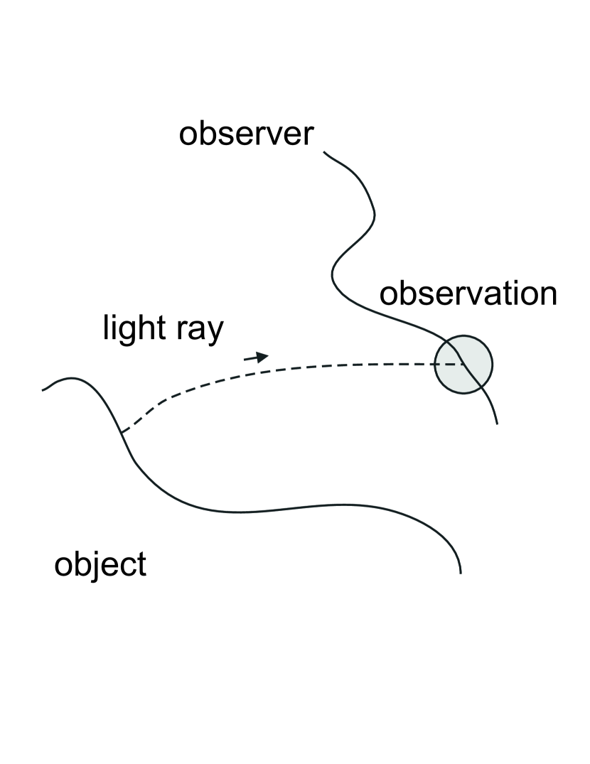
Figure 2: Four constituents of an astronomical event: 1) motion of the observed object, 2) motion of the observer, 3) propagation of an electromagnetic signal from the observed object to the observer, 4) the process of observation.

Let us first outline general principles of relativistic modeling of astronomical observations. General scheme is represented on Fig. 1. Starting from general theory of relativity, any other metric theory of gravity or PPN formalism one should define at least one relativistic 4-dimensional reference system covering the region of space-time where all the processes constituting particular kind of astronomical observations are located. Typical astronomical observation depicted on Fig. 2 consists of four constituents: motion of an observer, motion of an observed object, light progagation and the process of observation. Each of these four constituents should be modeled in the relativistic framework. The equations of motion of both the observed object and the observer relative to the chosen reference system should be derived and a method to solve these equations should be found. Typically the equations of motion are second-order ordinary differential equations and numerical integration with suitable initial or boundary conditions can be used to solve them. Astrometric information on the object can be read off the electromagnetic signals propagating from the object to the observer. Therefore, the corresponding equations of light propagation relative to the chosen reference system should be derived and solved. The equations of motion of the object and the observer and the equations of light propagation enable one to compute positions and velocities of the object, observer and the photon (light ray) with respect to the particular reference system at a given moment of its coordinate time, provided that the positions and velocities at some initial epoch are known. However, these positions and velocities obviously depend on the used reference system. On the other hand, the results of observations cannot depend on the reference system used to theoretically model the observations. Therefore, it is clear that one more step of the modeling is needed: a relativistic description of the process of observation. This part of the model allows one to compute a coordinate-independent theoretical prediction of the observables starting from the coordinate-dependent position and velocity of the observer and, in some cases, the coordinate velocity of the electromagnetic signal at the point of observation.

Mathematical techniques to derive the equations of motion of the observed object and the observer, to formulate the equations of light propagation and to find the description of the process of observation in the relativistic framework are well known and will be discussed below. These three parts can now be combined into relativistic models of observables. The models give an expression for each observable under consideration as a function of a set of parameters. These parameters can then be fitted to observational data using some kind of parameter estimation scheme (e.g. least squares or other estimators). The sets of certain estimated parameters appearing in the relativistic models of observables represent astronomical reference frames.

Note that reference system is a purely mathematical construction (a chart) giving “names” to space-time events. In contrast to this a reference frame is some materialization of a reference system. In astronomy usually the materialization is realized in a form of a catalogue (or ephemeris) containing positions of some celestial objects relative to the reference system under consideration. Any reference frame (a catalogue, an ephemeris, etc) is defined only through the reference system(s) used to construct physical models of observations.

It is very important to understand at this point that the relativistic models contain parameters which are defined only in the chosen reference system(s) and are thus coordinate-dependent. A good example of such coordinate-dependent parameters are the coordinates and velocities of various objects (e.g. major planets or the satellite) at some epoch. On the other hand, from the physical point of view any reference system covering the region of space-time under consideration can be used to describe physical phenomena within that region, and we are free to choose the reference system to be used to model the observations. However, reference systems, in which mathematical description of physical laws is simpler than in others, are more convenient for practical calculations. Therefore, one can use the freedom to choose the reference system to make the parametrization as convenient and reasonable as possible (e.g. one prefers the parameters to have a simpler time dependence).

For modeling of physical phenomena localized in some sufficiently small region of space (e.g. in the vicinity of a massless observer or a gravitating body) one can construct a so-called local reference system where the gravitational influence of the outer world is effaced as much as possible in accordance with the Einstein equivalence principle. In the local reference system of a material system the gravitational field of the outer matter manifests itself in the form of tidal gravitational potential. First, the Solar system as a whole can be considered as one single body, and a reference system can be constructed where the gravitational influence of the matter situated outside of the Solar system can be described by a tidal potential. That tidal potential (mainly due to the influence of the Galaxy) is utterly small and can be then neglected for most purposes. Such a reference system is often called barycentric reference system of the Solar system. It can be used far beyond the Solar system and is suitable to describe the dynamics of the Solar system (motion of planets and spacecraft relative to the barycenter of the Solar system) as well as to model the influence of the gravitational field of the Solar system on the light rays propagating from remote sources to an observer. Second, the corresponding local reference system can be constructed for the Earth. Such a geocentric reference system is convenient to model the geocentric motion of Earth satellites, the rotational motion of the Earth itself, etc. Underlying theory and technical details concerning local reference systems have been discussed in a series of papers by Brumberg and Kopeikin (Kopeikin, 1988; Brumberg & Kopeikin, 1989a, b; Brumberg, 1991, see also Klioner & Voinov (1993)) and by Damour, Soffel, & Xu (1991, 1992, 1993, 1994). IAU (2001) has recently recommended the use of a particular form of the barycentric and local geocentric reference systems for modeling of astronomical observations. These two standard relativistic reference systems are called Barycentric Celestial Reference System (BCRS) and Geocentric Celestial Reference System (GCRS). Coordinate time $t$ of the BCRS is called Barycentric Coordinate Time (TCB). Coordinate time $T$ of the GCRS is called Geocentric Coordinate Time (TCG). According to the IAU notations, throughout this paper the spatial coordinates of the BCRS will be designated as $x$ while those of the GCRS as $X$.

Both Brumberg-Kopeikin and Damour-Soffel-Xu theories are based on Einstein’s general relativity theory. It is clear, however, that one of the important goals of the future astrometric missions is to test general relativity. The model presented in this paper will be given in the framework of the PPN formalism (see, e.g. Will, 1993) including two main parameters $\beta$ and $\gamma$ which characterize possible devitations of the physical reality from general relativity. Both parameters are equal to unity in general relativity. The theory of local reference systems with parameters $\beta$ and $\gamma$ has been constructed by Klioner & Soffel (1998b, 2000). Both that theory of local PPN reference systems and the model given in the present paper are constructed in such a way that for $\beta=\gamma=1$ all the formulas coincide with those which can be derived directly from the general-relativistic versions of the BCRS and GCRS recommended by IAU (2001).

3 General structure of the relativistic model of positional observation

The relativistic model of positional observations relates the observed direction of the light coming from a source to the coordinates of that source at the moment of emission. A set of the coordinate directions toward the source for different moments of time can be then used to obtain further parameters of the source describing its spatial position and spatial motion with respect to the BCRS (parallax and proper motion or barycentric orbital elements). It is convenient to divide the conversion of the observed directions into the coordinate ones into several steps. Let us introduce five vectors which will be used below: $s$ is the unit observed direction (the word “unit” means here and below that the formally Euclidean scalar product $\mbox{\boldmath$s$}\,\cdot\,\mbox{\boldmath$s$}=s^{i}\,s^{i}$ is equal to unity), $n$ is the unit tangent vector to the light ray at the moment of observation, $\sigma$ is the unit tangent vector to the light ray at $t=-\infty$, $k$ is the unit coordinate vector from the source to the observer, $l$ is the unit vector from the barycenter of the Solar system to the source (see Fig. 3). Note that the last four vectors are defined formally in the coordinate space of the BCRS and should not be interpreted as “Euclidean” vectors in some “Newtonian physical space”. For the same physical situation these vectors are different if different reference systems are used instead of the BCRS. The word “vector” is used here to refer to a set of three real numbers defined in the coordinate space of the BCRS, rather than to a geometric object. A slightly different meaning of $s$ is discussed in Section 5 below.

$\bullet$$\bullet$$\bullet$................................................................................................................................................................................................................................................................................................$l$...............................................................................................................................................................................................................................................................................................................................................................................................................................................................................................................................................................................................................................................................................................................................................................................................................................................................................................................................................................................................................................................................................................................................................................................................................................................................................................................................................................................................................................................................................................................................................................................................................................................................................................................................................................................................................................................................................................................................................................................................................................................................................................................................................................................................................................................................................................................................................................................................................................................................................................................................................................................................................................................................................................................................................................................................................................................................................................................................................................................................................................................................................................................................................................................................................................................................................................................................................................................................................................................................................................................................................................................................................$\sigma$sourcesource pathbarycenterobserver’s pathobserver................................................................................................................................................................................................................................................................................................$s$................................................................................................................................................................................................................................................................................................$k$................................................................................................................................................................................................................................................................................................$n$light path...........................................................................................................................................................................................................

Figure 3: Five principal vectors used in the model: $s$, $n$, $\sigma$, $k$, $l$. See text for further details.

Apart from the modeling of the motion of the observer which will be considered in the next Section, the model consists in subsequent transformations of these five vectors. Namely, the following effects should be subsequently considered:

• aberration (the effects related to the motion of the observer with respect to the barycenter of the Solar system): this converts the observed direction to the source $s$ into the unit BCRS coordinate direction of the light ray $n$ at the point of observation;

• gravitational light deflection for the source at infinity: this step converts $n$ into the unit direction of propagation $\sigma$ of the light ray infinitely far from the Solar system for $t\to-\infty$;

• coupling of the finite distance to the source and the gravitational light deflection in the gravitational field of the Solar system: this step converts $\sigma$ into the unit BCRS vector $k$ going from the source to the observer (note that as discussed below this step should be combined with the previous one for the sources situated within the Solar system);

• parallax: this step converts $k$ into the unit vector $l$ going from the barycenter of the Solar system to the source;

• proper motion: this step provides a reasonable parametrization of the time dependence of $l$ caused by the motion of the source with respect to the BCRS.

All these steps will be specified in detail in the following Sections. However, let us first clarify the question of time scales which should be used in the model. There are four time scales appearing in the model:

• proper time of the observer (satellite): $\tau_{o}$.

• proper time of the $i$th tracking station: $\tau^{(i)}_{\rm station}$.

• coordinate time $t={\hbox{\rm TCB}}$ of the BCRS (alternatively a scaled version of TCB called TDB can be used: ${\hbox{\rm TDB}}=(1-L_{B})\,{\hbox{\rm TCB}}$ with the current best estimate of the scaling constant $L_{B}\approx 1.55051976772\cdot 10^{-8}\pm 2\cdot 10^{-17}$ (Irwin & Fukushima, 1999; IAU, 2001)).

• coordinate time $T={\hbox{\rm TCG}}$ of the GCRS (alternatively a scaled version of TCG called TT can be used: ${\hbox{\rm TT}}=(1-L_{G})\,{\hbox{\rm TCG}}$, $L_{G}\equiv 6.969290134\cdot 10^{-10}$ being a defining constant (IAU, 2001)).

It is clear that the observational data (e.g. in the case of the scanning satellites like HIPPARCOS, GAIA and DIVA these are the projections of the vector $s$ on a local reference system of the satellite which rotates together with the satellite) are parametrized by the proper time of the satellite $\tau_{o}$. It is also clear that the final catalog containing positions, parallaxes and proper motions of the sources relative to the BCRS should be parametrized by TCB. The other two time scales (proper times of the tracking station(s) $\tau^{(i)}_{\rm station}$ and TCG) are used exclusively for orbit determination.

The transformation between the proper time of the satellite $\tau_{o}$ and TCB can be done by integrating the equation

$${d\,\tau_{o}\over dt}=1-{1\over c^{2}}\left({1\over 2}\,\dot{\mbox{\boldmath$x$}}_{o}^{2}+w(\mbox{\boldmath$x$}_{o})\right)+{\cal O}(c^{-4}),$$ (1)

where $\mbox{\boldmath$x$}_{o}$ and $\dot{\mbox{\boldmath$x$}}_{o}$ are the BCRS position and velocity of the satellite and $w(\mbox{\boldmath$x$}_{o})$ is the gravitational potential of the Solar system which can be approximated by

$$w(\mbox{\boldmath$x$}_{o})\approx\sum_{A}{GM_{A}\over|\mbox{\boldmath$r$}_{oA}|},$$ (2)

where $\mbox{\boldmath$r$}_{oA}=\mbox{\boldmath$x$}_{o}-\mbox{\boldmath$x$}_{A}$, $M_{A}$ is the mass of body $A$, and $\mbox{\boldmath$x$}_{A}=\mbox{\boldmath$x$}_{A}(t)$ is its barycentric position. Both higher-order multipole moments of all the bodies and additional relativistic terms are neglected in (2). The transformation between the proper time of a tracking station and TCG can be performed in a similar way. The transformation between TCG and TCB is given in the IAU Resolutions B1.3 (general post-Newtonian expression) and B1.5 (an expression for the accuracy of $5\cdot 10^{-18}$ in rate and 0.2 ps in amplitude of periodic effects) of IAU (2001). There are several analytical and numerical formulas for the position-independent part of the transformation (see, e.g. Fukushima, 1995; Irwin & Fukushima, 1999, and reference cited therein).

Although the use of the relativistic time scales described above is indispensable from the theoretical and conceptual points of view, from a purely practical point of view considerations of accuracy can be used here to simplify the model. However, this depends on the particular parameters of the mission and will be not analyzed here. In the following it is assumed that the observed directions $s$ are given together with the corresponding epochs of observation $t_{o}$ in TCB scale.

4 Motion of the satellite

It is well known that in order to compute the Newtonian aberration with an accuracy of 1 $\mu$as one needs to know the velocity of the observer with an accuracy of $\sim 10^{-3}$ m/s (see, e.g. ESA, 2000). This is a rather stringent requirement and special care must be taken to attain such an accuracy. Modeling of the satellite motion with such an accuracy is a difficult task involving complicated equations of motion which take into account various non-relativistic (Newtonian $N$-body force, radiation pressure, active satellite thrusters, etc.) as well as relativistic effects. Here some general recipe concerning the relativistic part of the modeling will be given. Both the non-relativistic parts of the model and a detailed study of the relativistic effects in the satellite motion are beyond the scope of the present paper.

In the relativistic model of positional observations developed in the following Sections it is assumed that the observations are performed from a space station or an Earth satellite whose position $\mbox{\boldmath$x$}_{o}$ relative to the BCRS is known for any moment of barycentric coordinate time $t$. For those satellites the orbits of which are not located in the vicinity of the Earth (this is the case for both GAIA and SIM) it is advantageous to model their motion directly in the BCRS. Since the mass of the satellite is too small to noticeably affect the motion of other bodies of the Solar system, the equations of geodetic motion in the BCRS can be used as equations of motion of the satellite. It is sufficient (at least in the relativistic part of the equations) to neglect here the multipole structure of the gravitating bodies as well as the gravitational field produced by the rotational motion of these bodies. Therefore, considering a system of $N$ bodies, each of which can be characterized by position $\mbox{\boldmath$x$}_{A}$, velocity $\dot{\mbox{\boldmath$x$}}_{A}$ and mass $M_{A}$, the equations of motion of the satellite read (Will, 1993; Klioner & Soffel, 2000)

$${d^{2}\over dt^{2}}\,\mbox{\boldmath$x$}_{o} = -\sum_{A}G\,{\cal M}_{A}\,{\mbox{\boldmath$r$}_{oA}\over|\mbox{\boldmath$r$}_{oA}|^{3}}$$ (3)

$$+{1\over c^{2}}\,\sum_{A}G\,{\cal M}_{A}\,{\mbox{\boldmath$r$}_{oA}\over|\mbox{\boldmath$r$}_{oA}|^{3}}\,\Biggl{\{}(2\beta-1)\sum_{B\neq A}{G\,{\cal M}_{B}\over|\mbox{\boldmath$r$}_{AB}|}$$

$$\phantom{+{1\over c^{2}}\,\sum_{A}G\,{\cal M}_{A}\,{\mbox{\boldmath$r$}_{oA}\over|\mbox{\boldmath$r$}_{oA}|^{3}}\,\Biggl{\{}}+2(\gamma+\beta)\sum_{B}{G\,{\cal M}_{B}\over|\mbox{\boldmath$r$}_{oB}|}$$

$$\phantom{+{1\over c^{2}}\,\sum_{A}G\,{\cal M}_{A}\,{\mbox{\boldmath$r$}_{oA}\over|\mbox{\boldmath$r$}_{oA}|^{3}}\,\Biggl{\{}}+{3\over 2}{{\left(\mbox{\boldmath$r$}_{oA}\cdot\dot{\mbox{\boldmath$x$}}_{A}\right)}^{2}\over|\mbox{\boldmath$r$}_{oA}|^{2}}$$

$$\phantom{+{1\over c^{2}}\,\sum_{A}G\,{\cal M}_{A}\,{\mbox{\boldmath$r$}_{oA}\over|\mbox{\boldmath$r$}_{oA}|^{3}}\,\Biggl{\{}}-{1\over 2}\sum_{B\neq A}G\,{\cal M}_{B}\,{\mbox{\boldmath$r$}_{oA}\,\cdot\,\mbox{\boldmath$r$}_{AB}\over|\mbox{\boldmath$r$}_{AB}|^{3}}$$

$$\phantom{+{1\over c^{2}}\,\sum_{A}G\,{\cal M}_{A}\,{\mbox{\boldmath$r$}_{oA}\over|\mbox{\boldmath$r$}_{oA}|^{3}}\,\Biggl{\{}}-(1+\gamma)\,\dot{\mbox{\boldmath$x$}}_{A}\,\cdot\,\dot{\mbox{\boldmath$x$}}_{A}-\gamma\,\dot{\mbox{\boldmath$x$}}_{o}\,\cdot\,\dot{\mbox{\boldmath$x$}}_{o}$$

$$\phantom{+{1\over c^{2}}\,\sum_{A}G\,{\cal M}_{A}\,{\mbox{\boldmath$r$}_{oA}\over|\mbox{\boldmath$r$}_{oA}|^{3}}\,\Biggl{\{}}+2(1+\gamma)\,\dot{\mbox{\boldmath$x$}}_{o}\,\cdot\,\dot{\mbox{\boldmath$x$}}_{A}\Biggr{\}}$$

$$+{1\over c^{2}}\,\sum_{A}G\,{\cal M}_{A}\,{\dot{\mbox{\boldmath$x$}}_{o}-\dot{\mbox{\boldmath$x$}}_{A}\over|\mbox{\boldmath$r$}_{oA}|^{3}}\,\biggl{\{}2(1+\gamma)\,\dot{\mbox{\boldmath$x$}}_{o}\,\cdot\,\mbox{\boldmath$r$}_{oA}-(2\gamma+1)\,\dot{\mbox{\boldmath$x$}}_{A}\,\cdot\,\mbox{\boldmath$r$}_{oA}\biggr{\}}\,$$

$$-{1\over c^{2}}\,\left(2\gamma+{3\over 2}\right)\,\sum_{A}{G\,{\cal M}_{A}\over|\mbox{\boldmath$r$}_{oA}|}\,\sum_{B\neq A}G\,{\cal M}_{B}\,{\mbox{\boldmath$r$}_{AB}\over|\mbox{\boldmath$r$}_{AB}|^{3}}+{\cal O}(c^{-4}),$$

where $\mbox{\boldmath$r$}_{oA}=\mbox{\boldmath$x$}_{o}-\mbox{\boldmath$x$}_{A}$, $\mbox{\boldmath$r$}_{AB}=\mbox{\boldmath$x$}_{A}-\mbox{\boldmath$x$}_{B}$, and a dot denotes the total time derivative with respect to $t={\hbox{\rm TCB}}$: e.g. $\dot{\mbox{\boldmath$x$}}_{o}={d\over dt}\,\mbox{\boldmath$x$}_{o}(t)$.

The observations of the satellite itself performed to determine its orbit (typically range and Doppler tracking) should be also modeled in the relativistic framework: (1) the positions of the observing stations should be defined in the GCRS and then transformed into the BCRS, (2) the description of the signal propagation between the satellite and the observing stations must take into account the corresponding relativistic effects in the BCRS (the Shapiro effect, the relativistic Doppler effects, etc.), (3) the difference between the proper time scales of the satellite and the observing sites and the coordinate time of the BCRS must also be taken into account. A detailed description of these steps is beyond the scope of the present paper. The final result of the orbit determination procedure is the BCRS position $\mbox{\boldmath$x$}_{o}$ and velocity $\dot{\mbox{\boldmath$x$}}_{o}$ of the satellite as a function of $t={\hbox{\rm TCB}}$.

If the satellite is close enough to the Earth (geostationary or lower) it is advantageous to model its motion in the GCRS. The structure of the equations of motion of a satellite with respect to the GCRS can be written as

$${d^{2}\over dT^{2}}\,\mbox{\boldmath$X$}_{o} = \mbox{\boldmath$\Phi$}_{\rm E}+\mbox{\boldmath$\Phi$}_{\rm el}+{1\over c^{2}}\left(\mbox{\boldmath$\Phi$}_{\rm coup}+\mbox{\boldmath$\Phi$}_{\rm mg}+\mbox{\boldmath$\Phi$}_{\rm SEP}\right)+{\cal O}(c^{-4}),$$ (4)

where $\mbox{\boldmath$\Phi$}_{\rm E}$ is the acceleration due to the gravitational field of the Earth, $\mbox{\boldmath$\Phi$}_{\rm coup}$ is the Earth-third body coupling term, $\mbox{\boldmath$\Phi$}_{\rm el}$ is the “gravito-electric” part (independent of the velocity of the satellite) of the tidal influence of external bodies (this formally includes the Newtonian tidal force), $\mbox{\boldmath$\Phi$}_{\rm mg}$ is the purely relativistic “gravito-magnetic” part (depending on the velocity of the satellite) of the tidal influence of external bodies, and, finally, $\mbox{\boldmath$\Phi$}_{\rm SEP}$ is the additional acceleration due to possible violation of the strong equivalence principle in alternative theories of gravity ($\mbox{\boldmath$\Phi$}_{\rm SEP}\equiv 0$ in general relativity where the PPN parameters $\beta=\gamma=1$). The main relativistic terms in $\mbox{\boldmath$\Phi$}_{\rm E}$ come from the spherically symmetric part of the Earth’s gravitational field and can be formally derived in the framework of the Schwarzschild solution for the Earth considered to be isolated. This main relativistic effect is recommended to be taken into account in the IERS Conventions (IERS, 1996, , Chapter 11). Explicit formulas for the right-hand side of (4) can be found in Section VIII of Klioner & Soffel (2000) in the framework of the PPN formalism with parameters $\beta$ and $\gamma$. The same equations in the framework of general relativity were derived by Klioner & Voinov (1993), Damour, Soffel, & Xu (1994) and by Brumberg & Kopeikin (1989b).

If Eq. (4) is used to represent the motion of the satellite, the whole process of the orbit determination can be performed directly in the GCRS. Again the orbit determination observations should be consistently modeled in the relativistic framework: both the coordinates of the stations and the position of the satellite should be described in the GCRS, the propagation of the electromagnetic signals should be adequately modeled in the GCRS, the proper time of the satellite, that of the tracking stations and TCG should be properly converted into each other when needed. The result of the orbit determination process is the GCRS coordinates of the satellite $\mbox{\boldmath$X$}_{o}$ and its velocity ${d\over dT}\,\mbox{\boldmath$X$}_{o}$ as a function of $T={\hbox{\rm TCG}}$. In order to be used in the model of positional observations given below these coordinates must be transformed into the corresponding BCRS coordinates (see IAU, 2001; Klioner & Soffel, 2000):

$$\mbox{\boldmath$X$}_{o}=\mbox{\boldmath$r$}_{oE}+{1\over c^{2}}\left({1\over 2}\,\mbox{\boldmath$v$}_{E}\,(\mbox{\boldmath$v$}_{E}\cdot\mbox{\boldmath$r$}_{oE})+\gamma\,w_{\rm ext}(\mbox{\boldmath$x$}_{E})\,\mbox{\boldmath$r$}_{oE}+\gamma\,\mbox{\boldmath$r$}_{oE}\,(\mbox{\boldmath$a$}_{E}\cdot\mbox{\boldmath$r$}_{oE})-{1\over 2}\,\gamma\,\mbox{\boldmath$a$}_{E}\,|\mbox{\boldmath$r$}_{oE}|^{2}\right)+{\cal O}(c^{-4}),$$ (5)

where $\mbox{\boldmath$r$}_{oE}=\mbox{\boldmath$x$}_{o}-\mbox{\boldmath$x$}_{E}$, and $\mbox{\boldmath$x$}_{E}$, $\mbox{\boldmath$v$}_{E}$ and $\mbox{\boldmath$a$}_{E}$ are the BCRS position, velocity and acceleration of the Earth, and $w_{\rm ext}(\mbox{\boldmath$x$}_{E})$ is the gravitational potential of the Solar system except for that of the Earth evaluated at the geocenter. It is easy to estimate that the relativistic effects in (5) may amount to $\sim 1$ m for $|\mbox{\boldmath$r$}_{oE}|\sim 50000$ km. The GCRS velocity of the satellite can be transformed into the corresponding BCRS velocity as (this formula can be derived by taking time derivative of (5) and using the TCG-TCB transformation (IAU, 2001; Klioner & Soffel, 2000))

$${d\over dT}\,\mbox{\boldmath$X$}_{o}=\delta\mbox{\boldmath$v$}_{o}+{1\over c^{2}}\biggl{(} \delta\mbox{\boldmath$v$}_{o}\,\left({1\over 2}\,|\mbox{\boldmath$v$}_{E}|^{2}+(1+\gamma)\,(w_{\rm ext}(\mbox{\boldmath$x$}_{E})+\mbox{\boldmath$a$}_{E}\cdot\mbox{\boldmath$r$}_{oE})+\mbox{\boldmath$v$}_{E}\cdot\delta\mbox{\boldmath$v$}_{o}\right)$$ (6)

$$+{1\over 2}\,\mbox{\boldmath$v$}_{E}\,(\mbox{\boldmath$v$}_{E}\cdot\delta\mbox{\boldmath$v$}_{o})+\gamma\,\mbox{\boldmath$r$}_{oE}\,(\mbox{\boldmath$a$}_{E}\cdot\delta\mbox{\boldmath$v$}_{o})-\gamma\,\mbox{\boldmath$a$}_{E}\,(\mbox{\boldmath$r$}_{oE}\cdot\delta\mbox{\boldmath$v$}_{o})$$

$$+{1\over 2}\,\mbox{\boldmath$a$}_{E}\,(\mbox{\boldmath$v$}_{E}\cdot\mbox{\boldmath$r$}_{oE})+{1\over 2}\,\mbox{\boldmath$v$}_{E}\,(\mbox{\boldmath$a$}_{E}\cdot\mbox{\boldmath$r$}_{oE})+\gamma\,{\dot{w}}_{\rm ext}(\mbox{\boldmath$x$}_{E})\,\mbox{\boldmath$r$}_{oE}$$

$$+\gamma\,\mbox{\boldmath$r$}_{oE}\,(\dot{\mbox{\boldmath$a$}}_{E}\cdot\mbox{\boldmath$r$}_{oE})-{1\over 2}\,\gamma\,\dot{\mbox{\boldmath$a$}}_{E}\,|\mbox{\boldmath$r$}_{oE}|^{2}\biggr{)}+{\cal O}(c^{-4}),$$

where $\delta\mbox{\boldmath$v$}_{o}=\dot{\mbox{\boldmath$x$}}_{o}-\mbox{\boldmath$v$}_{E}$ and $\dot{\mbox{\boldmath$a$}}_{E}={d\over dt}\mbox{\boldmath$a$}_{E}$. It is easy to see from (6) that for a geostationary satellite numerical difference between ${d\over dT}\,\mbox{\boldmath$X$}_{o}$ and $\delta\mbox{\boldmath$v$}_{o}$ is less than $10^{-4}$ m/s. Therefore, for the model with a final accuracy of $\sim 1$ $\mu$as the relativistic terms in (6) can be neglected, and one can use ${d\over dT}\,\mbox{\boldmath$X$}_{o}=\delta\mbox{\boldmath$v$}_{o}$.

Note that probably even for the goal accuracy of $10^{-3}$ m/s in the velocity of the satellite one can significantly simplify both the BCRS equations of motion (3) and those in the GCRS (4). However, this crucially depends on the particular orbit of the satellite and such an analysis will not be given here.

Let us also note that the rotational motion of the satellite should also be carefully modeled (for some missions the attitude of the satellite will be determined from the observational data produced by the satellite, but nevertheless a kind of theoretical modeling is still necessary). From the theoretical point of view in order to model the rotational motion of the satellite it is convenient to introduce a local kinematically-nonrotating reference system for the satellite with coordinates $(\tau_{o},\mbox{\boldmath$\xi$})$, where $\tau_{o}$ is the proper time of the satellite related to $t$ by (1) and $\xi$ are the spatial coordinates of the reference system related to those of BCRS by a transformation analogous to (5) (see Brumberg & Kopeikin, 1989a; Klioner, 1993; Klioner & Soffel, 1998a, for details on the local reference system of the satellite). The rotational motion of the satellite with respect to the axes $\xi$ is described by the post-Newtonian rotational equations of motion discussed by Damour, Soffel, & Xu (1993) for the case of general relativity and by Klioner & Soffel (1998b, 2000) in the framework of the PPN formalism. From the practical point of view, it is, however, clear that the largest relativistic effect in the rotational motion of the satellite with respect to remote stars is due to the geodetic (de Sitter) precession which amounts to $\sim 2$ $\mu$as per hour ($\sim 2\arcsec$ per century) for the satellites on a heliocentric orbit with the semi-major axis close to 1 AU (like GAIA and SIM) and $\sim 140$ $\mu$as per hour ($\sim 1.2\arcsec$ per year) for the satellites on a geostationary orbit (like HIPPARCOS or DIVA). Taking into account that the satellites will typically monitor and verify their attitude with the help of onboard gyroscopes and observations of specially selected stars, and that the precise attitude with respect to remote stars will be determined aposteriori from the processing of observational data, it is unlikely that such small relativistic effects could be of practical importance.

The rest of the relativistic model of positional observations is totally independent of the GCRS. It is only the orbit determination process (or at least a part of that process) which involves the use of the GCRS coordinates and concepts.

5 Aberration

The first step of the model is to get rid of the aberrational effects induced by the barycentric velocity of the observer. Let $s$ denote the unit direction ($\mbox{\boldmath$s$}\,\cdot\,\mbox{\boldmath$s$}=1$) toward the source as observed by the observer (satellite). Let $p$ be the BCRS coordinate velocity of the photon at the point of observation. Note that $p$ is directed roughly from the source to the observer. The unit BCRS coordinate velocity of the light ray $\mbox{\boldmath$n$}=\mbox{\boldmath$p$}/|\mbox{\boldmath$p$}|$ (this implies $\mbox{\boldmath$n$}\,\cdot\,\mbox{\boldmath$n$}=1$) can be then computed as (Klioner, 1991b; Klioner & Kopeikin, 1992)

$$\mbox{\boldmath$s$}=-\mbox{\boldmath$n$} + \,{1\over c}\,\mbox{\boldmath$n$}\,\times\,(\dot{\mbox{\boldmath$x$}}_{o}\,\times\,\mbox{\boldmath$n$})$$ (7)

$$+ {1\over c^{2}}\,\Biggl{\{}\,(\mbox{\boldmath$n$}\,\cdot\,\dot{\mbox{\boldmath$x$}}_{o})\ \mbox{\boldmath$n$}\,\times\,(\dot{\mbox{\boldmath$x$}}_{o}\,\times\,\mbox{\boldmath$n$})+{1\over 2}\,\dot{\mbox{\boldmath$x$}}_{o}\,\times\,(\mbox{\boldmath$n$}\,\times\,\dot{\mbox{\boldmath$x$}}_{o})\,\Biggr{\}}$$

$$+ {1\over c^{3}}\,\Biggl{\{}\left({(\mbox{\boldmath$n$}\,\cdot\,\dot{\mbox{\boldmath$x$}}_{o})}^{2}+(1+\gamma)\,w(\mbox{\boldmath$x$}_{o})\right)\ \mbox{\boldmath$n$}\,\times\,(\dot{\mbox{\boldmath$x$}}_{o}\,\times\,\mbox{\boldmath$n$})+{1\over 2}\,(\mbox{\boldmath$n$}\,\cdot\,\dot{\mbox{\boldmath$x$}}_{o})\ \dot{\mbox{\boldmath$x$}}_{o}\,\times\,(\mbox{\boldmath$n$}\,\times\,\dot{\mbox{\boldmath$x$}}_{o})\Biggr{\}}$$

$$+ {\cal O}(c^{-4}),$$

where $w(\mbox{\boldmath$x$}_{o})$ is the gravitational potential of the Solar system at the point of observation. This formula contains relativistic aberrational effects up to the third order with respect to $1/c$. One can check from (7) that condition $\mbox{\boldmath$n$}\,\cdot\,\mbox{\boldmath$n$}=1$ implies $\mbox{\boldmath$s$}\,\cdot\,\mbox{\boldmath$s$}={\cal O}(c^{-4})$. Because of the first-order aberrational terms (classical aberration) in order to attain the accuracy of 1 $\mu$as the BCRS coordinate velocity of the satellite must be known to an accuracy of $\sim 10^{-3}$ m/s. For a satellite with the BCRS velocity $|\dot{\mbox{\boldmath$x$}}_{o}|\sim 40$ km/s, the first-order aberration is of the order of 28″, the second-order one may amount to 3.6 mas, and the third-order effects are $\sim 1$ $\mu$as. Note also that the higher-order aberrational effects are nonlinear with respect to the velocity of the satellite and cannot be divided into additive pieces like “annual” and “diurnal” aberrations as it could be done with the first-order aberration for an Earth-bound observer. This is the reason why it is advantageous to use directly the BCRS velocity of the satellite.

Vector $s$ is defined in the kinematically non-rotating local satellite reference system $(\tau_{o},\mbox{\boldmath$\xi$})$ which is mentioned in the previous Section. As it was discussed in Section 7.1 of Klioner & Kopeikin (1992) this point of view is equivalent to the standard tetrad approach discussed, e.g. by Brumberg (1986). The same form of Eq. (7) can be derived both from the standard tetrad formalism (see, e.g. Brumberg, 1986; Klioner, 1991b) and from the considerations related to the local reference system of the satellite (Klioner & Kopeikin, 1992). Actual observations of a scanning astrometric satellite are referred to a reference system, spatial axes of which rigidly rotate with respect to $\xi$ so that the satellite’s attitude remains fixed in the rotating axes. The rotating axes $\overline{\mbox{\boldmath$\xi$}}$ are related to the kinematically non-rotating axes $\xi$ as

$$\overline{\xi}^{a}=P^{ab}(\tau_{o})\,\xi^{b},$$ (8)

where $P^{ab}$ is a time-dependent orthogonal matrix, which can be parametrized, e.g. by three Euler angles. These Euler angles define the attitude of the satellite with respect to the kinematically non-rotating axis and should be determined from observations and the corresponding modeling. Depending on the particular optical scheme of the scanning satellite rotational motion of the satellite can produce an additional measurable aberrational effect. A detailed analysis of this additional effect will be published elsewhere.

To clarify the origin of the terms in (7) proportional to the gravitational potential $w$ let us consider a fictitious observer, whose position coincides with that of the satellite at the moment of observation and whose velocity with respect to the BCRS is zero. The direction toward the source observed by this fictitious observer

$$\mbox{\boldmath$s$}^{\prime}=-\mbox{\boldmath$n$}+{\cal O}(c^{-4})$$ (9)

as can be calculated from (7) for $\dot{\mbox{\boldmath$x$}}_{o}=0$. On the other hand, the transformation between the directions toward the source observed by the two observers located at the same point of space-time can be derived from the usual Lorentz transformation which can be used in its closed form to speed up the practical calculations (F. Mignard 2000, private communication). The Lorentz transformation depends only on the velocity of one observer as seen by the other one $v$. Hence, using the Lorentz transformation in its closed form one gets

$$s = \left(\mbox{\boldmath$s$}^{\prime}+\left\{\,{\Gamma\over c\,}+\left[\,\Gamma-1\,\right]\,{\mbox{\boldmath$v$}\cdot\mbox{\boldmath$s$}^{\prime}\over|\mbox{\boldmath$v$}|^{2}}\,\right\}\,\mbox{\boldmath$v$}\,\right)\,{1\over\Gamma\,\left(1+\mbox{\boldmath$v$}\cdot\mbox{\boldmath$s$}^{\prime}/c\right)},$$ (10)

$$\Gamma = {1\over\sqrt{1-|\mbox{\boldmath$v$}|^{2}/c^{2}}}.$$ (11)

It is easy to show from (10) that $\mbox{\boldmath$s$}^{\prime}\,\cdot\,\mbox{\boldmath$s$}^{\prime}=1$ implies $\mbox{\boldmath$s$}\,\cdot\,\mbox{\boldmath$s$}=1$. The velocity of the satellite as measured by the fictitious observer $v$ can again be calculated either with the help of the tetrad formalism (e.g. Brumberg, 1986) or by considering the local reference system for the fictitious observer (Klioner & Kopeikin, 1992; Klioner, 1993). The latter line of arguments leads to an equation similar to (6) where one should put to zero the BCRS velocity of the fictitious observer (this corresponds to $\mbox{\boldmath$v$}_{E}=0$ in (6)), its BCRS acceleration ($\mbox{\boldmath$a$}_{E}=0$ in (6)) as well as the position of the satellite relative to the local reference system ($\mbox{\boldmath$r$}_{oE}=0$ in (6)). Therefore, one gets

$$\mbox{\boldmath$v$}=\dot{\mbox{\boldmath$x$}}_{o}\,\left(\,1+{1\over c^{2}}\,(1+\gamma)\,w(\mbox{\boldmath$x$}_{o})\,\right)+{\cal O}(c^{-4}).$$ (12)

It is this renormalization of the velocity of the satellite which leads to the $w$-dependent terms in (7). It is easy to check that formulas (9)–(12) are equivalent to (7).

Alternatively, it is easy to calculate a formula relating the observed angular distance $\varphi_{12}^{\rm obs}$ ($\cos\varphi_{12}^{\rm obs}=\mbox{\boldmath$s$}_{1}\cdot\mbox{\boldmath$s$}_{2}$) between two given sources to the coordinate angular distance $\varphi_{12}^{\rm coord}$ between them ($\cos\varphi_{12}^{\rm coord}=\mbox{\boldmath$n$}_{1}\cdot\mbox{\boldmath$n$}_{2}$):

$$\cos\varphi_{12}^{\rm obs}=\cos\varphi_{12}^{\rm coord}+\left(\cos\varphi_{12}^{\rm coord}-1\right) \Biggl{[} -\left(1+{1\over c^{2}}\,(1+\gamma)\,w(\mbox{\boldmath$x$}_{o})\right)\,{|\dot{\mbox{\boldmath$x$}}_{o}|\over c}\,(\cos\theta_{1}+\cos\theta_{2})$$ (13)

$$+{|\dot{\mbox{\boldmath$x$}}_{o}|^{2}\over c^{2}}\,(\cos^{2}\theta_{1}+\cos^{2}\theta_{2}+\cos\theta_{1}\,\cos\theta_{2}-1)$$

$$-{|\dot{\mbox{\boldmath$x$}}_{o}|^{3}\over c^{3}}\,(\cos\theta_{1}+\cos\theta_{2})\,(\cos^{2}\theta_{1}+\cos^{2}\theta_{2}-1)\Biggr{]}$$

$$+{\cal O}(c^{-4}),$$

where $\theta_{i}$ are the angles between the direction toward the $i$th source and the direction of the velocity $\dot{\mbox{\boldmath$x$}}_{o}$:

$$\cos\theta_{i} = -{1\over|\dot{\mbox{\boldmath$x$}}_{o}|}\mbox{\boldmath$n$}_{i}\,\cdot\,\dot{\mbox{\boldmath$x$}}_{o},\qquad i=1,2.$$ (14)

The terms in (7) and (13) proportional to $w$ are the largest terms of the third order. The third-order terms are of order 1 $\mu$as and, therefore, the potential $w$ can be approximated here by the potential of the spherically symmetric Sun

$$w(\mbox{\boldmath$x$}_{o})\approx{GM_{\rm sun}\over|\mbox{\boldmath$x$}_{o}-\mbox{\boldmath$x$}_{\rm Sun}|}.$$ (15)

A closed-form expression equivalent to (13) can be derived from (10):

$$1-\cos\varphi_{12}^{\rm obs} = \left(1-\cos\varphi_{12}^{\rm coord}\right)\,{1-\displaystyle{\left|\mbox{\boldmath$v$}\right|^{2}\over c^{2}}\over\displaystyle\left(1+{\left|\mbox{\boldmath$v$}\right|\over c}\,\cos\theta_{1}\right)\displaystyle\left(1+{\left|\mbox{\boldmath$v$}\right|\over c}\,\cos\theta_{2}\right)},$$ (16)

where $v$ is defined by (12).

For order-of-magnitude estimations it is also useful to derive a formula for the angular shift $\delta\theta$ of the source toward the apex of the satellite’s motion:

$$\delta\theta = {1\over c}\,|\dot{\mbox{\boldmath$x$}}_{o}|\,\sin\theta\ \left(1+{1\over c^{2}}\,(1+\gamma)\,w(\mbox{\boldmath$x$}_{o})+{1\over 4}\,{|\dot{\mbox{\boldmath$x$}}_{o}|^{2}\over c^{2}}\right)$$ (17)

$$-{1\over 4}\,{|\dot{\mbox{\boldmath$x$}}_{o}|^{2}\over c^{2}}\,\sin 2\theta+{1\over 12}\,{|\dot{\mbox{\boldmath$x$}}_{o}|^{3}\over c^{3}}\,\sin 3\theta+{\cal O}(c^{-4})$$

or in the closed form

$$\cos(\theta-\delta\theta)={{\cos\theta+\displaystyle{\left|\mbox{\boldmath$v$}\right|\over c}}\over{1+\displaystyle{\left|\mbox{\boldmath$v$}\right|\over c}\,\cos\theta}}.$$ (18)

Here $\theta$ is the angle between the direction toward the source and the direction of the satellite’s velocity $\cos\theta=-\mbox{\boldmath$n$}\,\cdot\,\mbox{\boldmath$v$}\,/\,|\mbox{\boldmath$v$}|=-\mbox{\boldmath$n$}\,\cdot\,\dot{\mbox{\boldmath$x$}}_{o}\,/\,|\dot{\mbox{\boldmath$x$}}_{o}|$.

6 Gravitational light deflection

The next step is to account for the gravitational light defection, that is to convert $n$ into the corresponding unit coordinate direction $k$ from the observed source at the moment of emission to the observer at the moment of observation. Here two different cases should be distinguished: (1) objects outside of the Solar system for which their finite distance from the origin of the BCRS plays [almost] no role for this step of the reduction scheme, and (2) Solar system objects, the finite distance of which must be taken into account. Let us first relate $n$ to the unit coordinate direction $\sigma$ of the light propagation infinitely far from the gravitating sources for $t\to-\infty$ and then consider the influence of the finite distance to the objects on the gravitational light deflection separately for these two classes of objects (Sections 6.1 and 6.2 below).

The Solar system is assumed here to be isolated. This means that the gravitational field produced by the matter outside of the Solar system is neglected. This assumption is well founded if the time dependence of the gravitational field produced outside of the Solar system is negligible. Otherwise the external gravitational field must be explicitly taken into account (e.g. for observations of edge-on binary stars, where the gravitational field of the companion can cause an additional time-dependent light deflection, or for astrometric microlensing events). Some of such cases will be discussed below in Section 11.

The equations of light propagation can be derived from the general-relativistic Maxwell equations (Misner, Thorne, & Wheeler, 1973). It is sufficient, however, to consider only the limit of geometric optics. The relativistic effects depending on wavelength (and therefore representing deviations from geometric optics) are much smaller than 1 $\mu$as in the Solar system (see, e.g. Mashhoon, 1974). In the limit of geometric optics the relativistic equations of light propagation can be written in the form

$$\mbox{\boldmath$x$}_{p}(t)=\mbox{\boldmath$x$}_{p}(t_{o})+c\,\mbox{\boldmath$\sigma$}\,(t-t_{o})+\Delta\mbox{\boldmath$x$}_{p}(t),$$ (19)

where $t_{o}$ is the moment of observation, $\mbox{\boldmath$x$}_{p}(t_{o})$ is the position of the photon at the moment of observation (this position obviously coincides with the position of the satellite at that moment $\mbox{\boldmath$x$}_{p}(t_{o})=\mbox{\boldmath$x$}_{o}(t_{o})$), $\sigma$ is the unit coordinate direction of the light propagation at the past null infinity ($\mbox{\boldmath$\sigma$}\cdot\mbox{\boldmath$\sigma$}=1$)

$$\mbox{\boldmath$\sigma$}=\lim_{t\to-\infty}{1\over c}\,\dot{\mbox{\boldmath$x$}}_{p}(t),$$ (20)

and $\Delta\mbox{\boldmath$x$}_{p}$ is the sum of all gravitational effects in the light propagation which satisfies the conditions

$$\Delta\mbox{\boldmath$x$}_{p}(t_{o}) = 0,$$ (21)

$$\lim\limits_{t\to-\infty}\Delta\dot{\mbox{\boldmath$x$}}_{p}(t) = 0.$$ (22)

From the BCRS metric (IAU, 2001) one can easily see that $\Delta\mbox{\boldmath$x$}_{p}(t)\sim{\cal O}(c^{-2})$ and ${1\over c}\,\Delta\dot{\mbox{\boldmath$x$}}_{p}(t)\sim{\cal O}(c^{-2})$.

Several effects in $\Delta\mbox{\boldmath$x$}_{p}$ should be apriori considered at the level of 1 $\mu$as: (1) the effects of the spherically symmetric part of the gravitational field of each sufficiently large gravitating body, (2) the effects due to the non-sphericity (mainly due to the quadrupole moments) of the bodies, (3) the effects caused by the gravitomagnetic field due to the translational motion of the bodies, (4) the effects caused by the gravitomagnetic field due to the rotational motion of the bodies. The reduction formulas for all there effects have been derived and discussed in detail by Brumberg, Klioner, & Kopejkin (1990); Klioner (1991a, b); Klioner & Kopeikin (1992).

Table 1 illustrates the maximal magnitudes of the various gravitational effects due to the Solar system bodies and the maximal angular distances between the source and the body at which the gravitational light deflection from that body should still be accounted for to attain the final accuracy of 1 $\mu$as. Note that the values in Table 1 are slightly different from those published by Brumberg, Klioner, & Kopejkin (1990); Klioner (2000). The reason for this discrepancy is that for Table 1 the best current estimates for the physical parameters of the Solar system bodies were taken from Weissman, McFadden & Johnson (1999), whereas the IAU (1976) system of astronomical constants was used for the previous publications.

One can see that the post-post-Newtonian terms attain 1 $\mu$as only within 53′ from the Sun and can be currently neglected in the case of space astrometry since none of the proposed satellites could observe so close to the Sun. For the same reason the effect due to the rotational motion of the Sun amounting to 0.7 $\mu$as for a grazing ray is unobservable. The largest observable effect due to the rotational motion is 0.2 $\mu$as for a light ray grazing Jupiter. Therefore, the effects due to the rotational motion of the bodies are also too small to be taken into account.

The largest contribution in $\Delta\mbox{\boldmath$x$}_{p}$ for Solar system applications comes from the spherically symmetric components of the gravitational fields of the massive bodies and can be calculated as

$$\Delta_{pN}\mbox{\boldmath$x$}_{p}(t) = -\sum_{A}\,{(1+\gamma)GM_{A}\over c^{2}}\,\biggl{(}\,\mbox{\boldmath$d$}_{A}\,{\cal I}_{A}\,+\mbox{\boldmath$\sigma$}\,{\cal J}_{A}\biggr{)},$$ (23)

$$\mbox{\boldmath$d$}_{A} = \mbox{\boldmath$\sigma$}\,\times\,(\mbox{\boldmath$r$}_{oA}\,\times\,\mbox{\boldmath$\sigma$}),$$ (24)

$${\cal I}_{A} = {1\over|\mbox{\boldmath$r$}_{A}|-\mbox{\boldmath$\sigma$}\cdot\mbox{\boldmath$r$}_{A}}-{1\over|\mbox{\boldmath$r$}_{oA}|-\mbox{\boldmath$\sigma$}\cdot\mbox{\boldmath$r$}_{oA}},$$ (25)

$${\cal J}_{A} = \log{|\mbox{\boldmath$r$}_{A}|+\mbox{\boldmath$\sigma$}\cdot\mbox{\boldmath$r$}_{A}\over|\mbox{\boldmath$r$}_{oA}|+\mbox{\boldmath$\sigma$}\cdot\mbox{\boldmath$r$}_{oA}},$$ (26)

$$\mbox{\boldmath$r$}_{A} = \mbox{\boldmath$x$}_{p}(t)-\mbox{\boldmath$x$}_{A},$$ (27)

$$\mbox{\boldmath$r$}_{oA} = \mbox{\boldmath$x$}_{p}(t_{o})-\mbox{\boldmath$x$}_{A}=\mbox{\boldmath$x$}_{o}(t_{o})-\mbox{\boldmath$x$}_{A},$$ (28)

so that

$${1\over c}\,\Delta_{pN}\dot{\mbox{\boldmath$x$}}_{p}(t) = -\sum_{A}\,{(1+\gamma)GM_{A}\over c^{2}}\,\biggl{(}\,\mbox{\boldmath$d$}_{A}\,{1\over c}\,\dot{\cal I}_{A}\,+\mbox{\boldmath$\sigma$}\,{1\over c}\,\dot{\cal J}_{A}\biggr{)},$$ (29)

$${1\over c}\,\dot{\cal I}_{A} = {1\over|\mbox{\boldmath$r$}_{A}|\,(|\mbox{\boldmath$r$}_{A}|-\mbox{\boldmath$\sigma$}\cdot\mbox{\boldmath$r$}_{A})},$$ (30)

$${1\over c}\,\dot{\cal J}_{A} = {1\over|\mbox{\boldmath$r$}_{A}|},$$ (31)

where $\mbox{\boldmath$x$}_{A}$ is the position and $M_{A}$ is the mass of body A.

The positions of the bodies $\mbox{\boldmath$x$}_{A}$ are supposed to be constant in (23)–(31). In reality, however, the bodies are moving and this motion cannot be neglected in the calculation of light deflection. It is hardly possible to calculate analytically the light path in the gravitational field of an arbitrarily moving body without resorting to some approximations (see, however, Kopeikin & Schäfer, 1999). On the other hand, numerical integration of the equations of light propagation which could be used here as a remedy is too impractical for massive calculations necessary in astrometry. Let us, therefore, consider a Taylor expansion of $\mbox{\boldmath$x$}_{A}$:

$$\mbox{\boldmath$x$}_{A}(t)=\mbox{\boldmath$x$}^{\rm eph}_{A}(t_{A0})+\dot{\mbox{\boldmath$x$}}^{\rm eph}_{A}(t_{A0})\,(t-t_{A0})+{\cal O}(\ddot{\mbox{\boldmath$x$}}^{\rm eph}_{A}).$$ (32)

Note that here $\mbox{\boldmath$x$}^{\rm eph}_{A}(t_{A0})$ and $\dot{\mbox{\boldmath$x$}}^{\rm eph}_{A}(t_{A0})$ are the actual position and velocity of body $A$ taken from an ephemeris for some moment $t_{A0}$, while $\mbox{\boldmath$x$}_{A}(t)$ is the model for the position of body $A$ to be used for the approximate calculation of the light propagation. One can integrate the equations of motion for a light ray using (32) for the coordinates of the gravitating body. The solution was first derived by Klioner (1989) and describes the light propagation in the post-Newtonian approximation under the assumption that the gravitating bodies move with a constant velocity (only the effects linear with respect to velocity $\dot{\mbox{\boldmath$x$}}_{A}$ were taken into account, since formally the terms quadratic in $\dot{\mbox{\boldmath$x$}}_{A}$ are of post-post-Newtonian order ${\cal O}(c^{-4})$). However, expansion (32) has a free parameter $t_{A0}$ which can be used to minimize the error in the light propagation equations caused by the higher-order terms neglected in (32). From an analysis of the residual terms in the equations of light propagation proportional to the accelerations of the bodies Klioner & Kopeikin (1992) have shown that one reasonable choice which guarantee the residual effects to be negligible within the chosen approximation scheme is to set $t_{A0}$ equal to the moment of the closest approach $t^{\rm ca}_{A0}$ of the body and the photon

$$t^{\rm ca}_{A0} = \max\left(t_{e},t_{o}-\max\left(0,{\mbox{\boldmath$g$}\cdot(\mbox{\boldmath$x$}_{o}(t_{o})-\mbox{\boldmath$x$}^{\rm eph}_{A}(t_{o}))\over c\,|\mbox{\boldmath$g$}|^{2}}\right)\right),$$ (33)

$$g = \mbox{\boldmath$\sigma$}-{1\over c}\,\dot{\mbox{\boldmath$x$}}^{\rm eph}_{A}(t_{o}),$$ (34)

where $t_{e}$ is the time of emission of the light ray by the source (for sources located outside of the Solar system one can put $t_{e}=-\infty$ so that the outer ’$\max$’ in (33) can be omitted).

Recently an advanced formalism to integrate the equations of light propagation in the field of arbitrarily moving gravitating bodies has been developed by Kopeikin & Schäfer (1999) and Kopeikin & Mashhoon (2002). The authors suggest to use the solution of the Einstein field equations in the form of retarded potentials so that the positions of the gravitating bodies are computed for the retarded moment of time

$$t^{\rm r}_{A0}=t_{o}-{1\over c}\,|\mbox{\boldmath$x$}_{o}(t_{o})-\mbox{\boldmath$x$}^{\rm eph}_{A}(t^{r}_{A0})|,$$ (35)

and derive rigorous laws of the light propagation in the gravitational field of arbitrarily moving point masses in the first post-Minkowskian approximation (i.e. all the terms of order ${\cal O}(G^{2})$ are neglected). Using their rigorous approach the authors prove, however, that if the positions and velocities of the bodies are calculated at $t^{\rm r}_{A0}$ the effects due to the accelerations of the gravitating bodies as well as those proportional to the second and higher orders of velocities $\dot{\mbox{\boldmath$x$}}_{A}$ are much smaller than 1 $\mu$as for Solar system applications and thereby completely negligible for our model. On the other hand, if the effects due to the accelerations and those of the second and higher orders with respect to the velocities are neglected, so that each body is supposed to move with a constant velocity the formulas for $\Delta\mbox{\boldmath$x$}_{p}(t)$ derived by (Klioner, 1989; Klioner & Kopeikin, 1992) and those derived by (Kopeikin & Schäfer, 1999) coincide. If the bodies are supposed to move uniformly and rectilinearly and only the first-order terms with respect of the velocities are taken into account, the resulting solution for the light propagation can be considered as a numerical approximation to the rigorous solution derived by Kopeikin & Schäfer (1999). The parameter $t_{A0}$ remains a free parameter of this approximate solution. The approach due to Kopeikin & Schäfer (1999) does not prove that the choice $t_{A0}=t^{\rm r}_{A0}$ gives minimal residual terms in such an approximate solution. It is not clear which moment $t^{\rm r}_{A0}$ or $t^{\rm ca}_{A0}$ is numerically more advantageous to use in (32). However, if the effects explicitly proportional to $\dot{\mbox{\boldmath$x$}}_{A}$ are taken into account to compute the light path, the difference between the solutions for $t_{A0}=t^{\rm ca}_{A0}$ and for $t_{A0}=t^{\rm r}_{A0}$ in the gravitational field of the Solar system is several orders of magnitude lower than 1 $\mu$as.

The effect explicitly proportional to $\dot{\mbox{\boldmath$x$}}_{A}$ has been investigated in detail by Klioner (1989), Klioner & Kopeikin (1992) and Kopeikin & Schäfer (1999). If the position of the body is taken for $t_{A0}=t^{\rm ca}_{A0}$ or $t_{A0}=t^{\rm r}_{A0}$ this effect in the light deflection can be estimated as $\delta_{T^{\star}}\sim{1\over c}\,|\dot{\mbox{\boldmath$x$}}_{A}|\,\delta_{pN}$, where $\delta_{pN}$ is the deflection induced by the spherically symmetric field of the body. According to Table 1, $\delta_{T^{\star}}$ may amount to 0.8 $\mu$as for a light ray grazing Jupiter and only 0.1 $\mu$as in the case of the Sun. However, $\delta_{pN}$ attains its maximal value when the impact parameter of the light ray is much smaller than the distances between the gravitating body and the points of emission and observation. For this case one can prove that $\delta_{T^{\star}}\sim{1\over c}\,\left(\mbox{\boldmath$\sigma$}\cdot\dot{\mbox{\boldmath$x$}}_{A}\right)\,\delta_{pN}$. For the special case of an observer situated near the Earth orbit the cosine factor in $\mbox{\boldmath$\sigma$}\cdot\dot{\mbox{\boldmath$x$}}_{A}$ reduces the effects produced by Jupiter and Saturn in their orbital motion by a factor of at least 4 and 6, respectively. Therefore, the effects explicitly proportional to the velocities of the bodies can be neglected in our model.

If the effects due to the velocity of the body are completely neglected, we effectively use a constant value

$$\mbox{\boldmath$x$}_{A}(t)=\mbox{\boldmath$x$}_{A}(t_{A0})$$ (36)

for the coordinates of the bodies. Numerical simulations show that in the gravitational field of the Solar system the difference of the light deflection angle calculated using $t_{A0}=t^{\rm ca}_{A0}$ and that using $t_{A0}=t^{\rm r}_{A0}$ in (36) does not exceed 0.01 $\mu$as. Therefore, for practical purposes both $t^{\rm ca}_{A0}$ and $t^{\rm r}_{A0}$ can be used and $\mbox{\boldmath$x$}_{A}$ should be taken to be $\mbox{\boldmath$x$}_{A}(t^{\rm ca}_{A0})$ or $\mbox{\boldmath$x$}_{A}(t^{\rm r}_{A0})$ in (27)–(28) and all related formulas. Note, however, that, e.g. the use of the moment of reception $t_{o}$ instead of $t^{\rm ca}_{A0}$ or $t^{\rm r}_{A0}$ in (36) may lead to a significant error in the calculated gravitational light deflection. This maximal error of this kind can be roughly estimated as $|\mbox{\boldmath$r$}_{oA}|/L\,\cdot\,|\dot{\mbox{\boldmath$x$}}_{A}|/c\,\cdot\,\delta_{pN}$, where $L$ is the radius of the body and may amount to $\sim 10$ mas in the case of Jupiter.

It is to note that a number of smaller bodies should be also taken into account. For a spherical body with the mean density $\rho$, the light deflection is larger than $\delta$ if its radius

$$L\geq\left(\rho\over 1\,{\rm g/cm^{3}}\right)^{-1/2}\,\left(\delta\over 1\,\hbox{\rm$\mu$as}\right)^{1/2}\,624\,{\rm km}.$$ (37)

Therefore, at the level of 1 $\mu$as (and even 10 $\mu$as) one should additionally account for several largest satellites of the giant planets, Pluto and Charon, and also Ceres. The maximal values of the effects produced by these bodies are evaluated in Table 1. It is clear, however, that the gravitational light deflection due to these small bodies could be larger than 1 $\mu$as only if a source is observed very close to the corresponding body. The maximal angular distances at which this additional gravitational deflection should be taken into account are also given in Table 1.

Finally, the effects of the quadrupole fields of the giant planets should be taken into account if the angular distance between the planet and the object is smaller than the values given in the sixth column of Table 1. The corresponding reduction formulas for $\Delta_{Q}\mbox{\boldmath$x$}_{p}(t)$ and $\Delta_{Q}\dot{\mbox{\boldmath$x$}}_{p}(t)$ derived by Klioner (1991a) and Klioner & Kopeikin (1992) read

$$\Delta_{Q}\mbox{\boldmath$x$}_{p}(t) = {1\over 2\,c^{2}}\,(1+\gamma)\,G\,\sum_{A}\,\left(\mbox{\boldmath$\alpha$}_{A}\,{\cal U}_{A}+\mbox{\boldmath$\beta$}_{A}\,{\cal E}_{A}+\mbox{\boldmath$\gamma$}_{A}\,{\cal F}_{A}+\mbox{\boldmath$\delta$}_{A}\,{\cal V}_{A}\right),$$ (38)

$${\cal U}_{A} = {1\over|\mbox{\boldmath$d$}_{A}|}\,\left({1\over|\mbox{\boldmath$r$}_{A}|}\,{|\mbox{\boldmath$r$}_{A}|+\mbox{\boldmath$\sigma$}\cdot\mbox{\boldmath$r$}_{A}\over|\mbox{\boldmath$r$}_{A}|-\mbox{\boldmath$\sigma$}\cdot\mbox{\boldmath$r$}_{A}}-{1\over|\mbox{\boldmath$r$}_{oA}|}\,{|\mbox{\boldmath$r$}_{oA}|+\mbox{\boldmath$\sigma$}\cdot\mbox{\boldmath$r$}_{oA}\over|\mbox{\boldmath$r$}_{oA}|-\mbox{\boldmath$\sigma$}\cdot\mbox{\boldmath$r$}_{oA}}\right),$$ (39)

$${\cal E}_{A} = {\mbox{\boldmath$\sigma$}\cdot\mbox{\boldmath$r$}_{A}\over|\mbox{\boldmath$r$}_{A}|^{3}}-{\mbox{\boldmath$\sigma$}\cdot\mbox{\boldmath$r$}_{oA}\over|\mbox{\boldmath$r$}_{oA}|^{3}},$$ (40)

$${\cal F}_{A} = |\mbox{\boldmath$d$}_{A}|\,\left({1\over|\mbox{\boldmath$r$}_{A}|^{3}}-{1\over|\mbox{\boldmath$r$}_{oA}|^{3}}\right),$$ (41)

$${\cal V}_{A} = -{1\over|\mbox{\boldmath$d$}_{A}|^{2}}\,\left({\mbox{\boldmath$\sigma$}\cdot\mbox{\boldmath$r$}_{A}\over|\mbox{\boldmath$r$}_{A}|}-{\mbox{\boldmath$\sigma$}\cdot\mbox{\boldmath$r$}_{oA}\over|\mbox{\boldmath$r$}_{oA}|}\right),$$ (42)

$$\mbox{\boldmath$\alpha$}_{A} = 2\,\mbox{\boldmath$f$}_{A}-2\,(\mbox{\boldmath$f$}_{A}\cdot\mbox{\boldmath$\sigma$})\,\mbox{\boldmath$\sigma$}-(\mbox{\boldmath$g$}_{A}\cdot\mbox{\boldmath$\sigma$}+4\,\mbox{\boldmath$f$}_{A}\cdot\mbox{\boldmath$h$}_{A})\,\mbox{\boldmath$h$}_{A},$$ (43)

$$\mbox{\boldmath$\beta$}_{A} = 2\,(\mbox{\boldmath$f$}_{A}\cdot\mbox{\boldmath$\sigma$})\,\mbox{\boldmath$h$}_{A}+(\mbox{\boldmath$g$}_{A}\cdot\mbox{\boldmath$\sigma$}-\mbox{\boldmath$f$}_{A}\cdot\mbox{\boldmath$h$}_{A})\,\mbox{\boldmath$\sigma$},$$ (44)

$$\mbox{\boldmath$\gamma$}_{A} = 2\,(\mbox{\boldmath$f$}_{A}\cdot\mbox{\boldmath$\sigma$})\,\mbox{\boldmath$\sigma$}-(\mbox{\boldmath$g$}_{A}\cdot\mbox{\boldmath$\sigma$}-\mbox{\boldmath$f$}_{A}\cdot\mbox{\boldmath$h$}_{A})\,\mbox{\boldmath$h$}_{A},$$ (45)

$$\mbox{\boldmath$\delta$}_{A} = 2\,\mbox{\boldmath$g$}_{A}-4\,(\mbox{\boldmath$f$}_{A}\cdot\mbox{\boldmath$\sigma$})\,\mbox{\boldmath$h$}_{A}-(\mbox{\boldmath$g$}_{A}\cdot\mbox{\boldmath$\sigma$}-2\,\mbox{\boldmath$f$}_{A}\cdot\mbox{\boldmath$h$}_{A})\,\mbox{\boldmath$\sigma$},$$ (46)

$${1\over c}\,\Delta_{Q}\dot{x}^{i}_{p}(t) = {1\over 2\,c^{2}}\,(1+\gamma)\,G\,\sum_{A}\,\left(\mbox{\boldmath$\alpha$}_{A}\,{1\over c}\,\dot{\cal U}_{A}+\mbox{\boldmath$\beta$}_{A}\,{1\over c}\,\dot{\cal E}_{A}+\mbox{\boldmath$\gamma$}_{A}\,{1\over c}\,\dot{\cal F}_{A}+\mbox{\boldmath$\delta$}_{A}\,{1\over c}\,\dot{\cal V}_{A}\right),$$ (47)

$${1\over c}\,\dot{\cal U}_{A} = |\mbox{\boldmath$d$}_{A}|\,{2|\mbox{\boldmath$r$}_{A}|-\mbox{\boldmath$\sigma$}\cdot\mbox{\boldmath$r$}_{A}\over|\mbox{\boldmath$r$}_{A}|^{3}\,(|\mbox{\boldmath$r$}_{A}|-\mbox{\boldmath$\sigma$}\cdot\mbox{\boldmath$r$}_{A})^{2}},$$ (48)

$${1\over c}\,\dot{\cal E}_{A} = {|\mbox{\boldmath$r$}_{A}|^{2}-3(\mbox{\boldmath$\sigma$}\cdot\mbox{\boldmath$r$}_{A})^{2}\over|\mbox{\boldmath$r$}_{A}|^{5}},$$ (49)

$${1\over c}\,\dot{\cal F}_{A} = -3\,|\mbox{\boldmath$d$}_{A}|\,{\mbox{\boldmath$\sigma$}\cdot\mbox{\boldmath$r$}_{A}\over|\mbox{\boldmath$r$}_{A}|^{5}},$$ (50)

$${1\over c}\,\dot{\cal V}_{A} = -{1\over|\mbox{\boldmath$r$}_{A}|^{3}},$$ (51)

where $\mbox{\boldmath$h$}_{A}=\mbox{\boldmath$d$}_{A}/|\mbox{\boldmath$d$}_{A}|$, $f^{i}_{A}=M_{ij}^{A}\,h^{j}_{A}$, $g^{i}_{A}=M_{ij}^{A}\,\sigma^{j}$, and $M_{ij}^{A}$ is the symmetric trace-free quadrupole moment of body A. From the point of view of the theory of relativistic local reference systems, the multipole structure of the gravitational field of a body is defined in the corresponding local reference system of that body. However, for the calculation of the gravitational light deflection due to the quadrupole field the relativistic effects in $M^{A}_{ij}$ can be neglected. Matrix $M^{A}_{ij}$ is symmetric and trace-free and has, therefore, five independent components which can be calculated from the second zonal harmonic coefficient $J^{A}_{2}$ (in the case of the giant planets other coefficients of the second order are negligible), the mass $M_{A}$ and the equatorial radius $L_{A}$ of the planet, and the equatorial coordinates $(\alpha^{A}_{\rm pole},\delta^{A}_{\rm pole})$ of the north pole of its figure axis:

$$M^{A}_{ij}=M_{A}\,L_{A}^{2}\,J_{2}^{A}\,\pmatrix{A&B&C\cr B&D&E\cr C&E&-A-D},$$ (52)

$$A = {1\over 3}-\cos^{2}\!\alpha^{A}_{\rm pole}\,\cos^{2}\!\delta^{A}_{\rm pole},$$ (53)

$$B = -{1\over 2}\sin 2\alpha^{A}_{\rm pole}\,\cos^{2}\!\delta^{A}_{\rm pole},$$ (54)

$$C = -{1\over 2}\cos\alpha^{A}_{\rm pole}\,\sin 2\delta^{A}_{\rm pole},$$ (55)

$$D = {1\over 3}-\sin^{2}\!\alpha^{A}_{\rm pole}\,\cos^{2}\!\delta^{A}_{\rm pole},$$ (56)

$$E = -{1\over 2}\sin\alpha^{A}_{\rm pole}\,\sin 2\delta^{A}_{\rm pole}.$$ (57)

Various post-Newtonian gravitational effects in the light propagation (e.g. $\Delta_{pN}\mbox{\boldmath$x$}_{p}$ and $\Delta_{Q}\mbox{\boldmath$x$}_{p}$) are additive and one can put

$$\Delta\mbox{\boldmath$x$}_{p}=\Delta_{pN}\mbox{\boldmath$x$}_{p}+\Delta_{Q}\mbox{\boldmath$x$}_{p}.$$ (58)

Note that any additional post-Newtonian effects can be added in (58) if needed (e.g. the effects of the rotational and/or translational motion of the gravitating bodies).

As first discussed by Klioner (1991a), the higher-order multipole moments of Jupiter and Saturn may produce a deflection larger than 1 $\mu$as, provided that the source is observed very close to the surfaces of the planets. It is easy to see that the maximal gravitational light deflection produced by the zonal spherical harmonics $J_{n}$ (all other harmonics are utterly small for the giant planets) can be estimated as $\delta_{J_{n}}\sim J_{n}\,\delta_{pN}$. Using modern values for $J_{n}$ of Jupiter and Saturn (Weissman, McFadden & Johnson, 1999, p. 342) one can check that it is only the effects of $J_{4}$ of Jupiter and Saturn which may exceed 1 $\mu$as. Namely, the effect of $J_{4}$ of Jupiter may amount to 10 $\mu$as and that of Saturn is not greater than 6 $\mu$as. The effect of $J_{n}$ decreases as $\cot^{n+1}\psi$ with the angular distance $\psi$ between the gravitating body and the source. Therefore, the effect of $J_{4}$ of Jupiter exceeds 1 $\mu$as only if the angular distance $\psi$ between the center of Jupiter and the source is smaller than 1.6 of the apparent angular radius of Jupiter (i.e. smaller than 24 – 39″ depending on the mutual configuration of Jupiter and the observer). For $J_{4}$ of Saturn $\psi$ should be less than 1.4 of the apparent radius (i.e. less than 10 – 14″ depending on the configuration). The influence of $J_{6}$ of Jupiter and Saturn also may exceed 1 $\mu$as if the real values of $J_{6}$ (which are known with a large uncertainty for both planets) are larger than the values given by Weissman, McFadden & Johnson (1999). If the observations so close to Jupiter and Saturn are to be processed, the reduction formulas for the effect of $J_{4}$ can be derived from formulas given by Kopeikin (1997).

Let us note also that, generally speaking, the standard expansion of the gravitational potential of a body in terms of spherical functions (with harmonic coefficients like $J_{n}$) converges only outside of the sphere encompassing the body. Therefore, in general case the calculation of the gravitational light deflection for a light ray passing between the encompassing sphere and the surface of a body requires some other representation of the body’s gravitational potential. As discussed above for the accuracy level of 1 $\mu$as the non-sphericity of the gravitational field must be taken into account for the giant planets only. Since the polar radii of the giant planets are significantly smaller than their equatorial radii, impact parameter may be smaller than the equatorial radius of the body and, therefore, smaller than the radius of the encompassing sphere. However, the gravitational fields of the giant planets are close to that of a homogeneous axisymmetrical ellipsoid $(x^{2}+y^{2})/a^{2}+z^{2}/c^{2}\leq 1$ with $c<a$, for which the gravitational potential can be expanded as (Antonov, Timoshkova & Kholshevnikov, 1988, p. 187)

$$U(r,\vartheta) = {G\,M\over r}\,\left(1-\sum_{n=1}^{\infty}\,\left({a\over r}\right)^{2n}\,J^{\rm el}_{2n}\,P_{2n}(\cos\vartheta)\right),$$ (59)

$$J^{\rm el}_{2n} = (-1)^{n+1}\,{3\over(2n+1)\,(2n+3)}\,\left(1-{c^{2}\over a^{2}}\right)^{n},$$ (60)

where $M$ is the mass of the ellipsoid, $P_{n}(x)$ is the Legendre polynomial of order $n$, and $r$ and $\vartheta$ are the radial distance and the co-latitude, respectively. It is easy to see that expansion (59)–(60) converges for $r\geq\sqrt{a^{2}-c^{2}}$. Therefore, this expansion converges everywhere outside the ellipsoid (i.e. for $r\geq c$) if $c\geq a/\sqrt{2}$. Inequality $c\geq a/\sqrt{2}$ is true for all the giant planets of the Solar system. Moreover, since the density of the giant planets is not constant, but gets larger for smaller $r$ one should expect that the actual values of $J_{2n}$ are smaller than those “predicted” by (60). For a few first coefficients $J_{2n}$ it can be explicitly seen: the actual values of $J_{2}$, $J_{4}$ and $J_{6}$ given by Weissman, McFadden & Johnson (1999) are a factor 1.7–3.3 smaller than the corresponding coefficients from (60). This means that the expansion (59) with the actual zonal harmonics $J_{2n}$ of a giant planet converges everywhere outside of that planet. Therefore, for the giant planets for any impact parameter of the light ray it is sufficient to consider the standard expansion of the gravitational potential in terms of spherical harmonics (or, equivalently, multipole moments) and take into account the first few coefficients as discussed above.

Coordinate velocity of the photon can be obtained by taking time derivative of (19):

$$\mbox{\boldmath$p$}\equiv{1\over c}\,\dot{\mbox{\boldmath$x$}}_{p}(t_{o})=\mbox{\boldmath$\sigma$}+{1\over c}\,\Delta\dot{\mbox{\boldmath$x$}}_{p}(t_{o}).$$ (61)

The unit coordinate direction of the light propagation at the moment of observation reads

$$\mbox{\boldmath$n$}={\mbox{\boldmath$p$}\over|\mbox{\boldmath$p$}|}.$$ (62)

Eqs. (61)–(62) are more convenient for numerical calculations than an analytical expansion of $n$ in terms of $\sigma$ and $\Delta\dot{\mbox{\boldmath$x$}}_{p}$ which can be derived by substituting (61) into (62) and expanding in powers of $c^{-1}$. However, the accuracy of 1 $\mu$as can be attained with the simplified first-order expansion of (61)–(62)

$$\mbox{\boldmath$n$}=\mbox{\boldmath$\sigma$}+{1\over c}\,\mbox{\boldmath$\sigma$}\,\times\,(\Delta\dot{\mbox{\boldmath$x$}}_{p}(t_{o})\,\times\,\mbox{\boldmath$\sigma$})$$ (63)

if the distance from the observer to the Sun (all other bodies play no role here) is larger than 0.035 AU which is the case for all currently proposed astrometrical missions. Therefore,

$$n = \mbox{\boldmath$\sigma$}+\delta\mbox{\boldmath$\sigma$}_{pN}+\delta\mbox{\boldmath$\sigma$}_{Q},$$ (64)

$$\delta\mbox{\boldmath$\sigma$}_{pN} = {1\over c}\,\mbox{\boldmath$\sigma$}\,\times\,(\Delta_{pN}\dot{\mbox{\boldmath$x$}}_{p}(t_{o})\,\times\,\mbox{\boldmath$\sigma$}),$$ (65)

$$\delta\mbox{\boldmath$\sigma$}_{Q} = {1\over c}\,\mbox{\boldmath$\sigma$}\,\times\,(\Delta_{Q}\dot{\mbox{\boldmath$x$}}_{p}(t_{o})\,\times\,\mbox{\boldmath$\sigma$}).$$ (66)

Using (29) one gets

$$\delta\mbox{\boldmath$\sigma$}_{pN}=-\sum_{A}\,{(1+\gamma)GM_{A}\over c^{2}}\,\,{\mbox{\boldmath$d$}_{A}\over|\mbox{\boldmath$d$}_{A}|^{2}}\,\left(1+\mbox{\boldmath$\sigma$}\cdot{\mbox{\boldmath$r$}_{oA}\over|\mbox{\boldmath$r$}_{oA}|}\right).$$ (67)

Hence the post-Newtonian deflection angle due to the spherically symmetric part of the gravitational field of body $A$ reads

$$\delta_{pN}={(1+\gamma)GM_{A}\over c^{2}\,|\mbox{\boldmath$r$}_{oA}|}\,\cot{\psi_{A}\over 2},$$ (68)

where $\psi_{A}$ is the angular distance between body $A$ and the source. It is this formula which was used to compute the data in the third column of Table 1. The effect of the quadrupole field $\delta\mbox{\boldmath$\sigma$}_{Q}$ can be calculated by substituting (47)–(51) and (43)–(46) with (52)–(57) into (66).

body	$\delta_{pN}$	$\psi_{\rm max}(1\hbox{\rm$\mu$as})$	$\psi_{\rm max}(10\hbox{\rm$\mu$as})$	$\delta_{Q}$	$\psi_{\rm max}(1\hbox{\rm$\mu$as})$	$\delta_{R}$	$\delta_{T^{*}}$	$\delta_{ppN}$	$\psi_{\rm max}(1\hbox{\rm$\mu$as})$
Sun	$1.75\cdot 10^{6}$	180°	180°	$\sim$1		0.7	0.1	11	53′
Mercury	83	9′	54″	—		—	—	—
Venus	493	4.5°	27′	—		—	—	—
Earth	574	178°/123°	154°/21°	0.6		—	—	—
Moon	26	9°/5°	49′/26′	—		—	—	—
Mars	116	25′	2.5′	0.2		—	—	—
Jupiter	16270	90°	11.3°	240	152″	0.2	0.8	—
Saturn	5780	17°	1.7°	95	46″	—	0.2	—
Uranus	2080	71′	7.1′	8	4″	—	—	—
Neptune	2533	51′	5′	10	3″	—	—	—
Ganymede	35	32″	4″
Titan	32	14″	2″
Io	31	19″	2″
Callisto	28	23″	3″
Europe	19	11″	1″
Triton	10	0.7″
Pluto	7	0.4″
Titania	2.8	0.2″
Oberon	2.4	0.2″
Rhea	1.9	0.3″
Charon	1.7	0.05″
Iapetus	1.6	0.2″
Ariel	1.4	0.1″
Ceres	1.2	0.3″
Dione	1.2	0.2″
Umbriel	1.2	0.1″

Table 1: Various gravitational effects in the light propagation in $\mu$as: $\delta_{pN}$ and $\delta_{ppN}$ are the post-Newtonian and post-post-Newtonian effects due to the spherically symmetric field of each body, $\delta_{Q}$ are the effects due to the quadrupole gravitational fields, $\delta_{R}$ and $\delta_{T^{*}}$ are the effects due to the gravitomagnetic fields caused by the rotational and translational motions of the bodies, respectively. The estimations of $\delta_{T^{*}}$ are given for the case when the coordinates of the gravitating bodies are taken at the moment of the closest approach of the body and the photon (see text). Symbol “—” means that the corresponding effect is smaller than 0.1 $\mu$as. Physical parameters of the bodies are taken from Weissman, McFadden & Johnson (1999). Because of the minimal Sun avoidance angle the influence of some bodies can neglected for certain missions (for GAIA, e.g. Mercury is too close to the Sun and can be neglected). The angle $\psi_{\rm max}(\delta)$ is the maximal angular distance between the body and the source at which the corresponding effect still attains $\delta$ (the smallest possible distance between the observer and each body is taken here; $\psi_{\rm max}(\delta)$ is smaller for larger distances). For these estimates the observer is supposed to be within a few million kilometers from the Earth orbit. For the Earth and the Moon two estimates are given: for a geostationary satellite and for a satellite at a distance of $10^{6}$ km from the Earth.

6.1 Coupling of the finite distance to the source and the gravitational deflection: Solar system objects

The next step is to convert $\sigma$ into the unit vector $k$ directed from the point of emission to the point of observation. Let $\mbox{\boldmath$x$}_{o}(t_{o})$ be the coordinate of the observer (satellite) at the moment of observation $t_{o}$ and $\mbox{\boldmath$x$}_{s}(t_{e})$ be the position of the source at the moment of emission $t_{e}$ of the signal which was observed at $\mbox{\boldmath$x$}_{o}(t_{o})$. The moment of emission $t_{e}$ is considered as a function of the moment of observation $t_{o}$ (see Section 8 for further discussion). Let us denote

$$\mbox{\boldmath$R$}=\mbox{\boldmath$x$}_{o}(t_{o})-\mbox{\boldmath$x$}_{s}(t_{e}),$$ (69)

$$\mbox{\boldmath$k$}(t_{o})={\mbox{\boldmath$R$}\over|\mbox{\boldmath$R$}|},$$ (70)

It is easy to see that vector $k$ is related to $\sigma$ as (Klioner, 1991a):

$$\mbox{\boldmath$\sigma$}=\mbox{\boldmath$k$}+{1\over|\mbox{\boldmath$R$}|}\,\mbox{\boldmath$k$}\,\times\,(\Delta\mbox{\boldmath$x$}_{p}(t_{e})\,\times\,\mbox{\boldmath$k$})+{\cal O}(c^{-4}).$$ (71)

In the case of a Solar system object (71) can be combined with (63) to get

$$n = \mbox{\boldmath$k$}+\delta\mbox{\boldmath$k$}_{pN}+\delta\mbox{\boldmath$k$}_{Q},$$ (72)

$$\delta\mbox{\boldmath$k$}_{pN} = \mbox{\boldmath$k$}\,\times\,\left(\left({1\over|\mbox{\boldmath$R$}|}\,\Delta_{pN}\mbox{\boldmath$x$}_{p}(t_{e})+{1\over c}\,\Delta_{pN}\dot{\mbox{\boldmath$x$}}_{p}(t_{o})\right)\,\times\,\mbox{\boldmath$k$}\right),$$ (73)

$$\delta\mbox{\boldmath$k$}_{Q} = \mbox{\boldmath$k$}\,\times\,\left(\left({1\over|\mbox{\boldmath$R$}|}\,\Delta_{Q}\mbox{\boldmath$x$}_{p}(t_{e})+{1\over c}\,\Delta_{Q}\dot{\mbox{\boldmath$x$}}_{p}(t_{o})\right)\,\times\,\mbox{\boldmath$k$}\right).$$ (74)

Hence,

$$\delta\mbox{\boldmath$k$}_{pN} = -\sum_{A}\,{(1+\gamma)GM_{A}\over c^{2}}\,{\mbox{\boldmath$R$}\times(\mbox{\boldmath$r$}_{eA}\times\mbox{\boldmath$r$}_{oA})\over|\mbox{\boldmath$R$}|\,|\mbox{\boldmath$r$}_{oA}|\,(|\mbox{\boldmath$r$}_{eA}|\,|\mbox{\boldmath$r$}_{oA}|+\mbox{\boldmath$r$}_{oA}\cdot\mbox{\boldmath$r$}_{eA})},$$ (75)

$$\mbox{\boldmath$r$}_{eA} = \mbox{\boldmath$x$}_{s}(t_{e})-\mbox{\boldmath$x$}_{A}.$$ (76)

The angle between vectors $k$ and $n$ due to $\delta\mbox{\boldmath$k$}_{pN}$ can be calculated as

$${(1+\gamma)GM_{A}\over c^{2}\,|\mbox{\boldmath$r$}_{oA}|}\,\tan{\phi\over 2},$$ (77)

where $\phi$ is the angle between vectors $\mbox{\boldmath$r$}_{eA}$ and $\mbox{\boldmath$r$}_{oA}$. Note that the angle (77) depends on the distance $|\mbox{\boldmath$r$}_{oA}|$ between the gravitating body and the point of observation and on $\phi$, but does not depend on the distance $|\mbox{\boldmath$r$}_{eA}|$ between the point of emission and the gravitating body. For a remote source $|\mbox{\boldmath$r$}_{eA}|\to\infty$ and one has $\phi=\pi-\psi_{A}$ so that (77) coincides with (68).

The effect of the quadrupole field $\delta\mbox{\boldmath$k$}_{Q}$ can be calculated by substituting (38)–(57) into (74).

For an object located in the Solar system a set of vectors $k$ calculated from the observed directions $s$ for several different moments of time $t_{o}$ allows one to determine the barycentric orbit of that object. Therefore, vector $k$ is the final result of the model for the Solar system objects.

6.2 Coupling of the finite distance to the source and the gravitational deflection: objects outside the Solar system

The only effect in $\Delta\mbox{\boldmath$x$}_{p}$ which should be taken into account here for the objects located outside of the Solar system (with $|\mbox{\boldmath$x$}_{s}|>1000$ AU) is the post-Newtonian gravitational deflection from the spherically symmetric part of the gravitational field of the Sun. In this case from (71) one gets

$$\sigma = \mbox{\boldmath$k$}-{(1+\gamma)\,GM_{\rm Sun}\over c^{2}|\mbox{\boldmath$R$}|}\,{|\mbox{\boldmath$R$}|+|\mbox{\boldmath$r$}_{oS}|-|\mbox{\boldmath$r$}_{eS}|\over|\mbox{\boldmath$r$}_{oS}\times\mbox{\boldmath$r$}_{eS}|^{2}}\,\mbox{\boldmath$R$}\times(\mbox{\boldmath$r$}_{oS}\times\mbox{\boldmath$r$}_{eS})+{\cal O}(c^{-4}),$$ (78)

$$\mbox{\boldmath$r$}_{eS} = \mbox{\boldmath$x$}_{s}(t_{e})-\mbox{\boldmath$x$}_{\rm Sun},$$ (79)

$$\mbox{\boldmath$r$}_{oS} = \mbox{\boldmath$x$}_{o}(t_{o})-\mbox{\boldmath$x$}_{\rm Sun}.$$ (80)

The angle between $\sigma$ and $k$ can be calculated as

$${(1+\gamma)GM_{\rm Sun}\over c^{2}\,|\mbox{\boldmath$r$}_{oS}|\,\sin\psi_{\rm Sun}}\,\left(1+a-\sqrt{1-2a\cos\psi_{\rm Sun}+a^{2}}\right)\approx{(1+\gamma)\,GM_{\rm Sun}\over c^{2}\,|\mbox{\boldmath$R$}|}\,\left(\cot{\psi_{\rm Sun}\over 2}+{\cal O}(a)\right),$$ (81)

where $a=|\mbox{\boldmath$r$}_{oS}|/|\mbox{\boldmath$R$}|$ and $\psi_{\rm Sun}$ is the angular distance between the source and the Sun. The effect attains 8.5 $\mu$as for a source situated at a distance of 1 pc and observed at the limb of the Sun. One can check that the angle between $k$ and $\sigma$ is larger than 1 $\mu$as if $|\mbox{\boldmath$x$}_{s}|\leq 8.5\,{\rm pc}$ and the source is observed within 2.3° from the Sun. If at least one of these conditions is violated (which is really the case for all currently proposed astrometric missions since no observations can be done so close to the Sun) one can put

$$\mbox{\boldmath$\sigma$}=\mbox{\boldmath$k$}.$$ (82)

Let us note that the requirement to calculate the gravitational effects with an accuracy of 1 $\mu$as puts a constrain on the accuracy of the planetary ephemerides (roughly speaking, one has to be able to calculate the impact parameter of the light ray with respect to each gravitating body with a sufficient accuracy). The required accuracy of the ephemerides depends also on the minimal allowed angular distance between the source and the gravitating body. For a grazing ray the barycentric position of Jupiter should be known with an accuracy of 4 km and those for the other planets with slightly lower accuracy. The barycentric position of the Sun should be known with an accuracy of about 400 m for a grazing ray, and with an accuracy of $\sim 6000$ km for the minimal allowed angular distance of $35\arcdeg$ as adopted for GAIA. Note that since the model involves relative positions of the satellite and the gravitating bodies, the barycentric position of the satellite must be known with at least the same accuracy, i.e. $\sim 4$ km (see Section 5.4 of ESA (2000) for other accuracy constrains).

7 Parallax

Only the sources situated outside of the Solar system will considered below. For the objects situated outside of the Solar system the next step of the model is to get rid of the parallax, that is to transform $k$ into the unit vector $l$ directed from the barycenter of the Solar system to the source

$$\mbox{\boldmath$l$}(t)={\mbox{\boldmath$x$}_{s}(t_{e})\over|\mbox{\boldmath$x$}_{s}(t_{e})|}.$$ (83)

Note that starting from this point further parametrization of vectors $k$ and $l$ formally coincides with what one could expect in the Newtonian framework. From the formal mathematical point of view these vectors may be considered as “Euclidean vectors” in 3-dimensional coordinate space formed by the spatial coordinates of the BCRS. It is important to understand, however, that this interpretation is only formal and that those vectors are not Euclidean vectors in some “underlying Euclidean physical space”, but rather integration constants for the equations of light propagations in the BCRS. These vectors are defined by the whole previous model of relativistic reduction and would change if the model is changed (e.g. if another relativistic reference system is used instead of the BCRS).

Here, the definitions of parallax, proper motion and radial velocity compatible with general relativity at a level of 1 $\mu$as (or better) are suggested. Although the definitions are quite simple and straightforward, their interpretation at such a high level of accuracy is rather unusual from the point of view of classical Newtonian astrometry. As it will be clear below parallax and proper motion are no longer two separate effects which can be considered independently of each other. The second-order parallaxes and proper motions as well as the effects resulting from the interaction between these two effects are important. Moreover, parallax, proper motion and other astrometric parameters are coordinate-dependent parameters defined in the BCRS, which is used as the relativistic reference system where the position and motion of the sources are described. Therefore, these parameters have some meaning only within a particular chosen model of relativistic reductions. That is why the whole relativistic model of positional observations must be considered to define these parameters and clarify their meaning.

Let us define several parameters. The parallax of the source is defined as

$$\pi(t_{o})={1\,{\rm AU}\over|\mbox{\boldmath$x$}_{s}(t_{e})|},$$ (84)

the parallactic parameter $\Pi$ is given by

$$\mbox{\boldmath$\Pi$}(t_{o})=\pi(t_{o})\ {\mbox{\boldmath$x$}_{o}(t_{o})\over 1\,{\rm AU}},$$ (85)

and finally the observed parallactic shift of the source is defined as

$$\mbox{\boldmath$\pi$}(t_{o})=\mbox{\boldmath$l$}(t_{o})\,\times\,(\mbox{\boldmath$\Pi$}(t_{o})\,\times\,\mbox{\boldmath$l$}(t_{o})).$$ (86)

With these definitions to sufficient accuracy one has

$$\mbox{\boldmath$k$}=-\mbox{\boldmath$l$}\,\left(1-{1\over 2}\,|\mbox{\boldmath$\pi$}|^{2}\right)+\mbox{\boldmath$\pi$}\,\left(1+\mbox{\boldmath$l$}\,\cdot\,\mbox{\boldmath$\Pi$}\right)+{\cal O}(\pi^{3}).$$ (87)

The second-order effects in (87) proportional to $\pi^{2}$ are less 3 $\mu$as if $|\mbox{\boldmath$x$}_{s}|\geq 1$ pc. For the accuracy of 1 $\mu$as the second-order terms can be safely neglected if $|\mbox{\boldmath$x$}_{s}|\geq 2$ pc.

8 Proper motion

The last step of the algorithm is to provide a reasonable parametrization of the time dependence of $l$ and $\pi$ caused by the motion of the source relative to the barycenter of the Solar system.

It is commonly known that in order to convert the observed proper motion and the observed radial velocity into true tangential and radial velocities of the observed object additional information is required. Since that information is not always available, the concepts of “apparent proper motion”, “apparent tangential velocity” and “apparent radial velocity” are suggested below. These concepts represent useful information about the observed object and should be distinguished from the “true tangential velocity” and “true radial velocity”. Definitions of all these concepts are discussed below.

In the present paper the following simple model for the coordinates of the source is adopted:

$$\mbox{\boldmath$x$}_{s}(t_{e})=\mbox{\boldmath$x$}_{s}(t_{e}^{\ 0})+\mbox{\boldmath$V$}\,\Delta t_{e}+{1\over 2}\,\mbox{\boldmath$A$}\,\Delta t_{e}^{\ 2}+{\cal O}(\Delta t_{e}^{\ 3}),$$ (88)

Here, $\Delta t_{e}=t_{e}-t_{e}^{\ 0}$, and $V$ and $A$ are the BCRS velocity and acceleration of the source evaluated at the moment of emission $t_{e}^{\ 0}$ corresponding the initial epoch of observation $t_{o}^{\ 0}$. This model allows one to consider single stars or components of gravitationally bounded systems, periods of which are much larger than the time span covered by observations. Depending on particular properties of the source and on the time span of observations higher-order terms in (88) can also be considered. It is also clear that in more complicated cases special solutions for binary stars, etc. should be considered. For objects in double or multiple systems for which it is possible to determine the orbit, Eq. (88) gives the coordinates of the center of mass of such a system. The obvious correction should be added to the right-hand side of (88) in order to account for the orbital motion of the object. This case will not be considered here. In this paper we confine ourselves to Eq. (88) only.

Substituting (88) into the definitions of $l$ and $\pi$ one gets

$$\pi(t_{o}) = \pi_{0}+{\dot{\pi}}_{0}\,\Delta t_{e}+{1\over 2}\,{\ddot{\pi}}_{0}\,\Delta t_{e}^{\ 2}+{\cal O}(\Delta t_{e}^{\ 3}),$$ (89)

$$\dot{\pi}_{0} = -\pi_{0}\,{\mbox{\boldmath$l$}_{0}\cdot\mbox{\boldmath$V$}\over|\mbox{\boldmath$x$}_{s}(t_{e}^{\ 0})|},$$ (90)

$$\ddot{\pi}_{0} = -\pi_{0}\,{\mbox{\boldmath$l$}_{0}\cdot\mbox{\boldmath$A$}\over|\mbox{\boldmath$x$}_{s}(t_{e}^{\ 0})|}-\pi_{0}\,|\dot{\mbox{\boldmath$l$}}_{0}|^{2}+2\,{\dot{\pi}_{0}^{\ 2}\over\pi_{0}},$$ (91)

$$\mbox{\boldmath$l$}(t_{o}) = \mbox{\boldmath$l$}_{0}+\dot{\mbox{\boldmath$l$}}_{0}\,\Delta t_{e}+{1\over 2}\,\ddot{\mbox{\boldmath$l$}}_{0}\,\Delta t_{e}^{\ 2}+{\cal O}(\Delta t_{e}^{\ 3}),$$ (92)

$$\dot{\mbox{\boldmath$l$}}_{0} = {1\over|\mbox{\boldmath$x$}_{s}(t_{e}^{\ 0})|}\,\mbox{\boldmath$l$}_{0}\times(\mbox{\boldmath$V$}\times\mbox{\boldmath$l$}_{0}),$$ (93)

$$\ddot{\mbox{\boldmath$l$}}_{0} = {1\over|\mbox{\boldmath$x$}_{s}(t_{e}^{\ 0})|}\,\mbox{\boldmath$l$}_{0}\times(\mbox{\boldmath$A$}\times\mbox{\boldmath$l$}_{0})-|\dot{\mbox{\boldmath$l$}}_{0}|^{2}\,\mbox{\boldmath$l$}_{0}+2\,{\dot{\pi}_{0}\over\pi_{0}}\,\dot{\mbox{\boldmath$l$}}_{0},$$ (94)

where $\pi_{0}=\pi(t_{o}^{\ 0})=1\ {\rm AU}/|\mbox{\boldmath$x$}_{s}(t_{e}^{\ 0})|$ and $\mbox{\boldmath$l$}_{0}=\mbox{\boldmath$l$}(t_{o}^{\ 0})=\mbox{\boldmath$x$}_{s}(t_{e}^{\ 0})/|\mbox{\boldmath$x$}_{s}(t_{e}^{\ 0})|$ are the parameters at the initial epoch of observation $t_{o}^{\ 0}$.

The signals emitted at moments $t_{e}^{\ 0}$ and $t_{e}$ are received by the observer at moments $t_{o}^{\ 0}$ and $t_{o}$, respectively. The corresponding moments of emission and reception are related by

$$c\,(t_{o}-t_{e})=|\mbox{\boldmath$x$}_{o}(t_{o})-\mbox{\boldmath$x$}_{s}(t_{e})|-\mbox{\boldmath$k$}(t_{o})\cdot\Delta\mbox{\boldmath$x$}_{p}(t_{o}),$$ (95)

and by a similar equation for the moments $t_{o}^{\ 0}$ and $t_{e}^{\ 0}$. The term proportional to $\Delta\mbox{\boldmath$x$}_{p}$ represents the gravitational signal retardation (the Shapiro effect) due to the gravitational field of the Solar system. For any source in the observed part of the universe the Shapiro effect due to the gravitational field of the Solar system is less than $10^{-3}$ s and can be safely neglected here. Let us denote $\Delta t_{o}=t_{o}-t_{o}^{\ 0}$ the time span of observations corresponding the time span $\Delta t_{e}=t_{e}-t_{e}^{\ 0}$ of emission. These two time intervals are related as

$$\Delta t_{e} = \left(1+{1\over c}\,\mbox{\boldmath$l$}_{0}\,\cdot\,\mbox{\boldmath$V$}\right)^{-1}\,\Delta t_{o}+{1\over c}\,\mbox{\boldmath$l$}_{0}\,\cdot\,\left(\mbox{\boldmath$x$}_{o}(t_{o})-\mbox{\boldmath$x$}_{o}(t_{o}^{\ 0})\right)\,\left(1+{1\over c}\,\mbox{\boldmath$l$}_{0}\,\cdot\,\mbox{\boldmath$V$}\right)^{-1}$$ (96)

$$-{1\over 2c}\,\left(\mbox{\boldmath$l$}_{0}\cdot\mbox{\boldmath$A$}+{|\mbox{\boldmath$l$}_{0}\times\mbox{\boldmath$V$}|^{2}\over|\mbox{\boldmath$x$}_{s}(t_{e}^{\ 0})|}\right)\,\Delta t_{o}^{\ 2}+\dots$$

Eq. (96) results from a double Taylor expansion of the first term on the right-hand side of (95) in powers of parallax $\pi$ and $\Delta t_{e}$. Many terms have been neglected here since they were estimated to produce negligible observable effects. Which terms of such an expansion are important depends on many factors. The constrains used here to derive (96) are: $\pi_{0}\leq 1\arcsec$, proper motion $|\dot{\mbox{\boldmath$l$}}_{0}|\leq 1\ \hbox{\rm$\mu$as}/{\rm s}\approx 32\arcsec/{\rm yr}$, accuracy of position determination for a single observation is not better than 1 $\mu$as, lifetime of the mission is not longer than 5 yr, the effects of acceleration $A$ of the object were supposed to be smaller than those of velocity $V$ (i.e. $\mbox{\boldmath$A$}<2\mbox{\boldmath$V$}/\Delta t_{e}$). For other constrains other terms in the expansion may become important.

The second term in (96) represents a quasi-periodic effect with an amplitude $\ \sim|\mbox{\boldmath$x$}_{o}|/c\approx 500$ s for a satellite located not too far from the Earth orbit. Below it will be shown that this term gives a significant periodic term in the apparent proper motion of the sources with sufficiently large proper motions.

It is easy to see from (89)–(94) that the time dependence of parallax and proper motion characterized by the parameters $\dot{\pi}_{0}$ and $\ddot{\mbox{\boldmath$l$}}_{0}$ can be used to determine the radial velocity of the source. This question has been recently investigated in full detail and applied to Hipparcos data by Dravins, Lindegren, & Madsen (1999). The tangential and radial components of the barycentric velocity $V$ of the source can be defined by

$$\mbox{\boldmath$V$}_{\rm tan}=\mbox{\boldmath$l$}_{0}\times(\mbox{\boldmath$V$}\times\mbox{\boldmath$l$}_{0}),$$ (97)

$$V_{\rm rad}=\mbox{\boldmath$l$}_{0}\cdot\mbox{\boldmath$V$}.$$ (98)

Eqs. (89)–(94) can be combined with (96) to get the time dependence of $l$ and $\pi$. Collecting the terms linear with respect to $\Delta t_{o}$ we get the definition of the apparent proper motion $\mbox{\boldmath$\mu$}_{\rm ap}$ and the corresponding apparent tangential velocity $\mbox{\boldmath$V$}^{\rm ap}_{\rm tan}$ as appeared in the linear term in $\mbox{\boldmath$l$}(t_{o})$, and the definition of the apparent radial velocity $V^{\rm ap}_{\rm rad}$ as appeared in the linear term in $\pi(t_{o})$:

$$\mbox{\boldmath$V$}^{\rm ap}_{\rm tan} = \mbox{\boldmath$l$}_{0}\times(\mbox{\boldmath$V$}\times\mbox{\boldmath$l$}_{0})\,\left(1+{1\over c}\,\mbox{\boldmath$l$}_{0}\,\cdot\,\mbox{\boldmath$V$}\right)^{-1}=\mbox{\boldmath$V$}_{\rm tan}\,\left(1+{1\over c}\,V_{\rm rad}\right)^{-1},$$ (99)

$$\mbox{\boldmath$\mu$}_{\rm ap} = {1\over|\mbox{\boldmath$x$}_{s}(t_{e}^{\ 0})|}\,\mbox{\boldmath$l$}_{0}\times(\mbox{\boldmath$V$}\times\mbox{\boldmath$l$}_{0})\,\left(1+{1\over c}\,\mbox{\boldmath$l$}_{0}\,\cdot\,\mbox{\boldmath$V$}\right)^{-1}=\pi_{0}\ {\mbox{\boldmath$V$}^{\rm ap}_{\rm tan}\over 1\ {\rm AU}},$$ (100)

$$V^{\rm ap}_{\rm rad} = \mbox{\boldmath$l$}_{0}\cdot\mbox{\boldmath$V$}\,\left(1+{1\over c}\,\mbox{\boldmath$l$}_{0}\,\cdot\,\mbox{\boldmath$V$}\right)^{-1}=V_{\rm rad}\,\left(1+{1\over c}\,V_{\rm rad}\right)^{-1}.$$ (101)

With these definitions the simplest possible models for $\pi(t_{o})$ and $\mbox{\boldmath$l$}(t_{o})$ read (the higher-order terms are neglected here in order to make this example more transparent):

$$\pi(t_{o})=\pi_{0}-\pi_{0}^{2}\,{V^{\rm ap}_{\rm rad}\over 1\ {\rm AU}}\,\Delta t_{o}+\dots,$$ (102)

$$\mbox{\boldmath$l$}(t_{o})=\mbox{\boldmath$l$}_{0}+\mbox{\boldmath$\mu$}_{\rm ap}\,\Delta t_{o}+\mbox{\boldmath$\mu$}_{\rm ap}\,{1\over c}\,\biggl{(}[\mbox{\boldmath$x$}_{o}(t)-\mbox{\boldmath$x$}_{o}(t_{0})]\,\cdot\,\mbox{\boldmath$l$}_{0}\biggr{)}+\dots.$$ (103)

Factor $\left(1+c^{-1}\,\mbox{\boldmath$l$}_{0}\,\cdot\,\mbox{\boldmath$V$}\right)^{-1}$ in (99)–(101) has been discussed by, e.g. Stumpff (1985) and Klioner & Kopeikin (1992). If vectors $\mbox{\boldmath$l$}_{0}$ and $V$ are nearly antiparallel and $|\mbox{\boldmath$V$}|$ is large, this factor may become large so that the apparent tangential and radial velocities may even exceed light velocity. This phenomenon is one of the well-known possible explanations of apparent superluminal motions.

The amplitude of the third term in (103) is about 170 $\mu$as for the Barnard’s star with its proper motion of $10.4\arcsec$ per year (see Brumberg, Klioner, & Kopejkin, 1990; Klioner & Kopeikin, 1992). In general the amplitude of this effect is approximately equal to the proper motion of the source during the time interval $\sim|\mbox{\boldmath$x$}_{o}|/c$ required for the light to propagate from the observer to the barycenter of the Solar system multiplied by cosine of the ecliptical latitude of the source. Therefore, for a satellite not too far from the Earth orbit where $|\mbox{\boldmath$x$}_{o}|/c\sim 500$ s, this effect exceeds 1 $\mu$as for all stars with the proper motion larger than $\sim 63$ mas/yr. This effect is closely related to the Roemer effect used in the 17th century to measure the light velocity. Its potential importance for astrometry was recognized by Schwarzschild (1894) and later discussed in detail by Stumpff (1985). The Roemer effect is a standard part of typical relativistic models for pulsar timing (see, e.g. Doroshenko & Kopeikin, 1990).

The apparent radial velocity $V^{\rm ap}_{\rm rad}$ can be immediately used to calculate the true radial velocity $V_{\rm rad}$. Therefore, if both the apparent tangential and apparent radial velocities are determined from observations one can immediately restore the true tangential velocity $\mbox{\boldmath$V$}_{\rm tan}$. However, even if it is not the case the apparent velocity $\mbox{\boldmath$V$}^{\rm ap}_{\rm tan}$ can be useful by itself. Note that the radial velocities measured by Doppler (spectral) observations are neither true nor apparent radial velocity in our terminology. The shift of spectral lines is affected by a number of factors not appearing in positional observations (various gravitational red shifts and Doppler effects; see, a detailed discussion e.g. by Kopeikin & Ozernoy (1999)). The relativistic effects induced by the motion of the satellite and by the gravitational field of the Solar system in the Doppler measurements are typically of the order of a few cm/s which is probably too small to be detectable by space astrometry missions (for example, GAIA will measure the Doppler shift of spectral lines with an accuracy of about 1 km/s). Therefore, it is only the intrinsic red shift due to local physics of the object which should be considered (see, e.g. Neill, 1996).

9 Summary of the model

Practical implementation of the model can be summarized as follows:

1. determine the orbit (the position $\mbox{\boldmath$x$}_{o}$ and the velocity $\dot{\mbox{\boldmath$x$}}_{o}$) of the satellite with respect to the BCRS (Section 4);

2. re-parametrize the observed directions $s$ by the coordinate time $t$ of the BCRS (to this end Eq. (1) should be numerically integrated along the orbit of the satellite);

3. use Eqs. (9)–(12) to convert the observed direction $s$ to the source into the unit BCRS direction $n$ of the light ray at the point of observation;

4. for the objects situated outside of the Solar system use Eqs. (64), (67), (66) with (47)–(51), (43)–(46) and (52)–(57), and (82) to convert $n$ into the unit BCRS direction $k$ from the source to the observer at the moment of observation; in order to judge if the light deflection due to a particular gravitating body should be considered here one can use Eq. (68) and/or the maximal angular distances given in Table 1;

5. for the Solar system objects use Eqs. (72), (75) and (74) with (38)–(57) to convert $n$ into $k$ (a set of vectors $k$ for several moments of time can be used to determine the BCRS orbit of the object which represents the final outcome for a Solar system body); Eqs. (68), (77) and/or the maximal angular distances given in Table 1 can be again used to judge if a particular gravitating body should be taken into account here;

6. use Eqs. (87) with (84)–(86) to take into account the parallax of the object and to convert $k$ into the unit BCRS direction $l$ from the barycenter of the Solar system to the source;

7. use an appropriate model for the time dependence of $l$ and possibly of the parallactic parameter $\pi$ to account for the proper motion of the source (a reasonable model for single sources is given in Section 8).

Figure 4: The structure of the model for different kinds of objects (see text).

The sequence of the steps of the model is depicted on Fig. 4.

10 The model for 0.1 $\mu$as

Since the technical accuracy of GAIA is expected to attain 4 $\mu$as for the stars with the magnitude of 12 mag and brighter, and the technical accuracy of SIM is also expected to attain the level of 3-4 $\mu$as, it is interesting to look at the relativistic model having an accuracy of 0.1 $\mu$as which guarantees that all systematic effects of the level of 1 $\mu$as are properly taken into account. The relativistic effects related to the gravitational potential of the Solar system bodies and to the motion of the observer with respect the barycenter of the Solar system can be modeled with the accuracy of 0.1 $\mu$as within the same scheme discussed above and summarized in the previous Section. The necessary changes to attain the accuracy of 0.1 $\mu$as are:

1. The barycentric velocity of the satellite should be known with an accuracy of $10^{-4}$ m/s. This also requires the use of Eq. (6) if the GCRS is used for orbit determination.

2. Some additional effects should be taken into account in the gravitational light deflection (see also Table 1):

   1. The effect explicitly proportional to the velocity of the bodies should be taken into account when observing within 8 angular radii of Jupiter or 2 angular radii of Saturn. As discussed in Section 6 the difference between $t^{\rm r}_{A0}$ and $t^{\rm ca}_{A0}$ still plays no role at this level of accuracy. The explicit formulas has been published by Klioner (1989), Klioner & Kopeikin (1992) and Kopeikin & Schäfer (1999).

   2. The effect of the rotational motion of Jupiter should be taken into account when observing within 1.4 of its apparent radius (i.e. within 42–69″ from the Jupiter’s center). The explicit formulas for this effect have been published by Klioner (1991a) and Klioner & Kopeikin (1992).

   3. The effect of $J_{4}$ of Jupiter exceeds 0.1 $\mu$as within 2.5 of its apparent radius (37–61″ from the Jupiter’s center); the same effect for Saturn exceeds 0.1 $\mu$as within 2.2 of its apparent radius (15–22″ from the Saturn’s center). The effect of $J_{6}$ (Weissman, McFadden & Johnson, 1999, p. 342) of both Jupiter and Saturn may exceed 0.1 $\mu$as within 1.3 of the apparent radii of each planet. The explicit formulas for the influence of $J_{4}$ and $J_{6}$ have been published by Kopeikin (1997).

   4. All the bodies, the radius $L$ of which

      $$L\geq\left(\rho\over 1\,{\rm g/cm^{3}}\right)^{-1/2}\,197\,{\rm km},$$ (104)

      where $\rho$ is the mean density of the body, can produce light deflection of order 0.1 $\mu$as and should be taken into account. This makes it quite difficult to reduce the observations near the ecliptic where a large number of small bodies satisfying this condition can be expected.

   5. The maximal angular distances at which the influence of a gravitating body should be taken into account should be increased as compared to Table 1 to meet the goal accuracy of 0.1 $\mu$as. The post-post-Newtonian light deflection attains 0.1 $\mu$as only for observations within 2.3° from the Sun and, therefore, can be neglected for the planned space missions.

   6. Coupling of the finite distance to the source and the gravitational deflection for sources located outside of the Solar system (Section 6.2) should be taken into account if $|\mbox{\boldmath$x$}_{s}|\leq 85$ pc and the source is observed within 22.7° from the Sun. Although for the current technical specifications of the planned space missions the effect can be neglected, it may become important since the Sun avoidance angle of $\sim 23\arcdeg$ is not technically impossible.

3. The second-order parallactic effects (Section 7) should be taken into account if $|\mbox{\boldmath$x$}_{s}|\leq 5.5$ pc.

4. The model for the proper motion (Section 8) should be correspondingly refined. In particular the third term in (103) becomes important for all the stars with the proper motion larger than $\sim 0.62$″/yr.

Note also that additional relativistic effects due to various gravitational fields generated outside of the Solar system (see Section 11 below and Kopeikin & Gwinn (2000)) become even more important at the level of 0.1 $\mu$as and should be thoroughly taken into account.

11 What is beyond the model

The relativistic model proposed above can be considered as a “standard” model suitable for all sources. This model allows one to reduce the observational data with an accuracy of 1 $\mu$as and restore positions and other parameters of the objects (e.g. their velocities) defined in the BCRS. The model properly takes into account the gravitational field of the Solar system, but ignores a number of possible effects which may be caused by the gravitational fields produced outside of the Solar system. Let us review some of these effects (see also Kopeikin & Gwinn, 2000).

The first additional effect to mention here is the so-called weak microlensing which is simply an additional gravitational deflection of the light coming from a distant source which is produced by the gravitational field of a visible or invisible object situated near the light path between the observed source and the observer. For applications in high-precision astrometry one should distinguish between microlensing events and microlensing noise. Microlensing event is a time dependent change of source’s position (and possibly its brightness) which is large and clear enough to be identified as such. Microlensing events can be used to determine physical properties of the lens so that the unperturbed path of the source can be restored at the end (e.g. Hosokawa et al., 1993, 1995; Høg, Novikov & Polnarev, 1995; Belokurov & Evans, 2002). In this sense microlensing events represent no fundamental problem for the future astrometric missions. On the other hand, microlensing noise comes from unidentified microlensing events (which are too weak or too fast to be detected as such). The number of such unidentified microlensing events will be clearly much higher than the number of identified ones. The microlensing noise results in stochastic changes of positions of the observed sources with unpredictable (but generally small) amplitude and to unpredictable moments of time. Therefore, microlensing noise can spoil the determination of positions, parallaxes and proper motions of the objects (Zhdanov, 1995; Zhdanov & Zhdanova, 1995; Hosokawa et al., 1997; Sazhin et al., 1998, 2001; Belokurov & Evans, 2002). It is currently not quite clear to what extent the microlensing noise produced by the objects of the Galaxy can deteriorate the resulting catalogs of the future astrometric missions. To clarify this question data simulations similar to those described by de Felice et al. (2000), but involving a model for microlensing with a realistic model for the Galaxy would be of much help. The first simulation of this kind has been performed by Belokurov & Evans (2002) who conclude that the microlensing noise presents no problem for GAIA. On the other hand, the accuracy level of $\sim 1$ $\mu$as seems to be close to a fundamental limit of astrometric accuracy, since at much higher accuracies the stochastic influence of microlensing noise becomes too strong so that in too many cases measurable relativistic deflection effects cannot be property taken into account (Sazhin et al., 1998, 2001).

In edge-on binary (or multiple) systems the gravitational light deflection due to the gravitational field of the companion may be observable. In the case of pulsar timing observations of binary pulsars this question has been thoroughly investigated by Doroshenko & Kopeikin (1995). It is clear that for companions with stellar masses the inclination of the orbit should be very close to 90° for the effect to be observable at the level of 1 $\mu$as. The formulas of Section 6.1 can be directly used here to calculate the effect in the first post-Newtonian approximation. If the lensing companion is a neutron star or a black hole it is necessary to investigate the lensing effect in the strong field regime and also consider secondary images (a detailed study of the strong-field-regime appearance of a star orbiting a Kerr black hole is given by Cunningham & Bardeen (1972, 1973)). Further investigation is necessary to estimate the probability to observe a binary system for which the gravitational lensing of the companion is important at the level of 1 $\mu$as.

Gravitational waves can in principle produce gravitational light deflection. Two cases should be distinguished here: 1) gravitational waves from binary stars and other compact sources and 2) stochastic primordial gravitational waves from the early universe. Gravitational waves from a single compact source were shown to produce an utterly small deflection which is hardly observable at the level of 1 $\mu$as (Kopeikin et al., 1999). However, the ensemble of compact sources of gravitational waves in the Galaxy (e.g. binary stars) may produce a larger cumulative effect which should be thoroughly estimated (see, e.g. (Kopeikin, 1999) for an attempt of such an estimation in pulsar timing measurements). The influence of primordial gravitational waves was analyzed by Pyne et al. (1996) and Gwinn et al. (1997). Although initially applied for VLBI, the method of these authors can be directly used for optical astrometry.

Finally, cosmological effects should be accounted for to interpret the derived parameters of the objects (e.g. the accuracy of parallaxes $\sigma_{\pi}=1$ $\mu$as allows one to measure the distance to the objects as far as $\sim 1$ Mpc away from the Solar system; see, e.g. Kristian & Sachs (1965) for a discussion of astrometric consequences of cosmology). It may be interesting here to construct the metric tensor of the BCRS with a cosmological solution as a background and analyze the effects of the background cosmology in such a reference system.

Last but not least, the observational accuracy of 1 $\mu$as together with the mission lifetime of at least 5 years allow one to see the apparent proper motions of quasars and other remote sources due to the acceleration of the Solar system barycenter relative to the center of the Galaxy (ESA, 2000, Section 1.8.10). These proper motions should be of order of $\sim 4$ $\mu$as/yr, if one assumes the Solar system to be on a circular orbit around the Galactic center.

References

- Antonov, Timoshkova & Kholshevnikov (1988) Antonov, V.A., Timoshkova, E.I., & Kholshevnikov, K.V. 1988, Introduction to the theory of the Newtonian Potential (Moscow: Nauka), in Russian
- Bienayme & Turon (2002) Bienayme, O., & Turon, C. 2002, GAIA: A European Space Project (Les Ulis: EDP Sciences)
- Belokurov & Evans (2002) Belokurov, V.A., & Evans, N.W. 2002, MNRAS, 331, 649
- Brumberg (1986) Brumberg, V.A. 1986, in Astrometric Techniques, ed. H.K. Eichhorn, & R.J. Leacock (Dordrecht: Reidel), 19
- Brumberg (1991) Brumberg, V.A. 1991, Essential Relativistic Celestial Mechanics (Bristol: Hilger)
- Brumberg, Klioner, & Kopejkin (1990) Brumberg, V.A., Klioner, S.A., & Kopejkin, S.M. 1990, in Inertial Coordinate System on the Sky, ed. J.H. Lieske & V.K. Abalakin (Dordrecht: Kluwer), 229
- Brumberg & Kopeikin (1989a) Brumberg, V.A., & Kopejkin, S.M. 1989a, in: Reference Frames, ed. J. Kovalevsky, I.I. Mueller, & B. Kołaczek (Dordrecht:Kluwer), 115
- Brumberg & Kopeikin (1989b) Brumberg, V.A., & Kopejkin, S.M. 1989b, Nuovo Cimento, 103B, 63
- Cunningham & Bardeen (1972) Cunningham, C.T., & Bardeen, J.M. 1972, ApJ, 173, L137
- Cunningham & Bardeen (1973) Cunningham, C.T., & Bardeen, J.M. 1973, ApJ, 183, 237
- Damour, Soffel, & Xu (1991) Damour, T., Soffel, M., & Xu, C. 1991, Phys. Rev. D, 43, 3273
- Damour, Soffel, & Xu (1992) Damour, T., Soffel, M., & Xu, C. 1992, Phys. Rev. D, 45, 1017
- Damour, Soffel, & Xu (1993) Damour, T., Soffel, M., & Xu, C. 1993, Phys. Rev. D, 47, 3124
- Damour, Soffel, & Xu (1994) Damour, T., Soffel, M., & Xu, C. 1994, Phys. Rev. D, 49, 618
- Dravins, Lindegren, & Madsen (1999) Dravins, D., Lindegren, L., & Madsen, S. 1999, A&A, 348, 1040
- de Felice et al. (2001) de Felice, F., Bucciarelli, B., Lattanzi, M.G., & Vecchiato, A. 2001, A&A, 373, 336
- de Felice et al. (1998) de Felice, F., Lattanzi, M.G., Vecchiato, A., & Bernacca, P.L. 1998, A&A, 332, 1133
- de Felice et al. (2000) de Felice, F., Vecchiato, A., Bucciarelli, B., Lattanzi, M.G., & Crosta, M. 2000, in Towards Models and Constants for Sub-Microarcsecond Astrometry, ed. K.J. Johnston, D.D. McCarthy, B.J. Luzum, & G.H. Kaplan (Washington: US Naval Observatory), 314
- Doroshenko & Kopeikin (1990) Doroshenko, O.V., & Kopeikin, S.M. 1990, AZh, 67, 986, in Russian
- Doroshenko & Kopeikin (1995) Doroshenko, O.V., & Kopeikin, S.M. 1995, MNRAS, 274, 1029
- ESA (2000) ESA, 2000, GAIA: Composition, Formation and Evolution of the Galaxy, Concept and Technology Study Report, Document ESA-SCI(2000)4, European Space Agency, Noordwijk
- Fukushima (1995) Fukushima, T. 1995, A&A, 294, 895
- Gwinn et al. (1997) Gwinn, C.R., Eubanks, T.M., Pyne, T., Birkinshaw, M., & Matsakis, D.N. 1997, ApJ, 485, 87
- Høg, Novikov & Polnarev (1995) Høg, E., Novikov, I.D., & Polnarev, A.G. 1995, A&A, 294, 287
- Hosokawa et al. (1993) Hosokawa, M., Ohnishi, K., Fukushima, T., & Takeuti, M. 1993, A&A, 278, L27
- Hosokawa et al. (1995) Hosokawa, M., Ohnishi, K., Fukushima, T., & Takeuti, M. 1995, in Astronomical and Astrophysical Objectivities of Sub-Milliarcsecond Optical Astrometry, ed. E. Høg, & P.K. Seidelmann (Dordrecht: Kluwer), 305
- Hosokawa et al. (1997) Hosokawa, M., Ohnishi, K., & Fukushima, T. 1997, AJ, 114, 1508
- IAU (2001) IAU 2001, Information Bulletin, 88 (errata in IAU Information Bulletin, 89)
- IERS (1996) IERS 1996, IERS Conventions, International Earth Rotation Service Technical Note 21, ed. D.D. McCarthy (Paris: Observatoire de Paris)
- Irwin & Fukushima (1999) Irwin, A.W. & Fukushima, T. 1999, A&A, 348, 642
- Klioner (1989) Klioner, S.A. 1989, Institute of Applied Astronomy, preprint No 6, in Russian
- Klioner (1991a) Klioner, S.A. 1991a, AZh, 68, 1046, in Russian (translated into English: Soviet Ast., 35, 523)
- Klioner (1991b) Klioner, S.A. 1991b, Ph.D. thesis, Institute of Applied Astronomy & St.Petersburg State University, in Russian
- Klioner (1993) Klioner, S.A. 1993, A&A, 279, 273
- Klioner (2000) Klioner, S.A. 2000, in Towards Models and Constants for Sub-Microarcsecond Astrometry, ed. K.J. Johnston, D.D. McCarthy, B.J. Luzum, & G.H. Kaplan (Washington: US Naval Observatory), 308
- Klioner & Kopeikin (1992) Klioner S.A., & Kopeikin, S.M. 1992, AJ, 104, 897
- Klioner & Soffel (1998a) Klioner, S.A., & Soffel, M. 1998a, A&A, 334, 1123
- Klioner & Soffel (1998b) Klioner, S.A., & Soffel, M.H. 1998b, Phys. Rev. D, 58, ID 084023
- Klioner & Soffel (2000) Klioner, S.A., & Soffel, M.H. 2000, Phys. Rev. D, 62, ID 024019
- Klioner & Voinov (1993) Klioner, S.A., & Voinov, A.V. 1993, Phys. Rev. D, 48, 1451
- Kopeikin (1988) Kopejkin, S.M. 1988, Celestial Mechanics, 44, 87
- Kopeikin (1997) Kopeikin, S.M. 1997, J. Math. Phys., 38, 2587
- Kopeikin (1999) Kopeikin, S.M. 1999, available as http://xxx.lanl.gov/abs/gr-qc/9903070
- Kopeikin & Ozernoy (1999) Kopeikin, S.M., & Ozernoy, L.M., 1999, ApJ, 523, 771
- Kopeikin et al. (1999) Kopeikin, S.M., Schäfer, G., Gwinn, C.R., & Eubanks, T.M. 1999, Phys. Rev. D, 59, ID 084023
- Kopeikin & Gwinn (2000) Kopeikin, S.M., & Gwinn, C. 2000, in Towards Models and Constants for Sub-Microarcsecond Astrometry, ed. K.J. Johnston, D.D. McCarthy, B.J. Luzum, & G.H. Kaplan (Washington: US Naval Observatory), 303
- Kopeikin & Schäfer (1999) Kopeikin, S.M., & Schäfer, G. 1999, Phys. Rev. D, 60, ID 124002
- Kopeikin & Mashhoon (2002) Kopeikin, S.M., & Mashhoon, B. 2002, Phys. Rev. D, 65, ID 064025
- Kopeikin et al. (2000) Kopeikin, S.M., Shuygina, N., Vasiliev, M., Yagudina, E., & Yagudin, L. 2000, in Towards Models and Constants for Sub-Microarcsecond Astrometry, ed. K.J. Johnston, D.D. McCarthy, B.J. Luzum, & G.H. Kaplan (Washington: US Naval Observatory), 320
- Kristian & Sachs (1965) Kristian, J., & Sachs, R.K. 1965, ApJ, 143, 379
- Mashhoon (1974) Mashhoon, B. 1974, Nature, 250, 316
- Misner, Thorne, & Wheeler (1973) Misner, C.W., Thorne, K.S., Wheeler, J.A. 1973, Gravitation (San Francisco: Freeman)
- Neill (1996) Neill, R.I. 1996, AJ, 111, 2000
- Perryman et al. (2001) Perryman, M. A. C., et al. 2001, A&A, 369, 339
- Pyne et al. (1996) Pyne, T., Gwinn, C.R, Birkinshaw, M., Eubanks, T.M., & Matsakis, D.N. 1996, ApJ, 465, 566
- Reasenberg et al. (1988) Reasenberg, R.D., et al. 1988, AJ, 96, 1731
- Sazhin et al. (1998) Sazhin, M.V., Zharov, V.E., Volynkin, A.V., & Kalinina, T.A. 1998, MNRAS, 300, 287
- Sazhin et al. (2001) Sazhin, M.V., Zharov, V.E., & Kalinina, T.A. 2001, MNRAS, 323, 952
- Schwarzschild (1894) Schwarzschild, K. 1894, Astr. Nachr., 136, No. 3246, 81
- Shao (1998) Shao, M. 1998, in Astronomical Interferometry, ed. R.D. Reasenberg, Proc. SPIE, 3350, 536
- Stumpff (1985) Stumpff, P. 1985, A&A, 144, 232
- Walter et al. (1986) Walter, H. G., Mignard, F., Hering, R., Froeschlé, M., & Falin, J. L. 1986, Manuscripta Geodaetica, 11, 103
- Weissman, McFadden & Johnson (1999) Weissman, P.R., McFadden, L.-A., Johnson, T.V. (eds.) 1999, Encyclopedia of the Solar System (San Diego: Academic Press)
- Will (1993) Will, C. M. 1993, Theory and experiment in gravitational physics (Cambridge: Cambridge University Press)
- Zhdanov (1995) Zhdanov, V.I. 1995, in Astronomical and Astrophysical Objectivities of Sub-Milliarcsecond Optical Astrometry, ed. E. Høg, & P.K. Seidelmann (Dordrecht: Kluwer), 295
- Zhdanov & Zhdanova (1995) Zhdanov, V.I., & Zhdanova, V.V. 1995, A&A, 299, 321