Gradient Particle Magnetohydrodynamics

Abstract

We introduce Gradient Particle Magnetohydrodynamics (GPM), a new Lagrangian method for magnetohydrodynamics based on gradients corrected for the locally disordered particle distribution. The development of a numerical code for MHD simulation using the GPM algorithm is outlined. Validation tests simulating linear and nonlinear sound waves, linear MHD waves, advection of magnetic fields in a magnetized vortex, hydrodynamical shocks, and three-dimensional collapse are presented, demonstrating the viability of an MHD code using GPM. The characteristics of a GPM code are discussed and possible avenues for further development and refinement are mentioned. We conclude with a view of how GPM may complement other methods currently in development for the next generation of computational astrophysics.

1 Introduction

Computer modeling of astrophysical fluids often requires the accurate representation of densities and other fluid quantities which vary over several orders of magnitude due to the inherent compressibility of the interstellar medium. This challenge has often been met by the use of Lagrangian particle methods to simulate astrophysical fluid flow. The “particles” in a simulation represent fluid elements. When the fluid is compressed to high densities, the particles—points where we know information about the fluid—flow with the fluid, resulting in increased resolution in the dense regions. The relative computational ease with which resolution is enhanced in a regions of increased density has made Lagrangian methods very attractive to astrophysicists. Grid-based methods entail great computational complexity in order to attain such a selective resolution enhancement. The drawback of Lagrangian methods is that it is more difficult to achieve the desirable conservation properties characteristic of grid-based methods.

Smoothed Particle Hydrodynamics (SPH) is a Lagrangian technique that has seen widespread use since its introduction by Lucy (1977) and Monaghan and Gingold (1977) two decades ago. Although the technique does not provide a solution to high accuracy, SPH has proven extremely valuable through its ability to yield solutions to many problems that other computational methods could not possibly tackle.

Today, computational astrophysicists are seeking to extend the limits of applicability of their techniques. Those using grid-based methods have turned to Adaptive Mesh Refinement (AMR) to push the limits of these high-accuracy methods to allow larger variation in density. For those employing SPH codes, the inclusion of magnetic fields has become a priority to apply the method to a wider range of phenomena in which the dynamical effect of magnetic fields cannot be neglected.

Gradient Particle Magnetohydrodynamics (GPM) is a new algorithm introduced here for Lagrangian simulation of magnetohydrodynamics (MHD). It is, essentially, an algorithm for correctly calculating the gradient of fluid quantities in the presence of particle disorder. SPH, a Monte Carlo technique, fails to stably include magnetic fields because of the small-scale noise inherent in Monte Carlo methods. GPM determines the gradients of fluid quantities exactly, rather than statistically, and therefore is not susceptible to the same magnetic tension instability arising in SPH.

We begin, in Section 2, with a discussion of the problems with existing particle methods for hydrodynamics and describe the GPM algorithm which solves these problems. In Section 3, we describe the application of the GPM algorithm to the equations of MHD and discuss viscosity, magnetic divergence, and advanced features to be implemented in the code. Analytical estimates of the error of this method are presented in Section 2.2.1. Section 4 presents the validation tests performed with the new GPM technique. Issues arising from the validation tests are discussed in Section 5 and concluding remarks are made in Section 6.

2 Properties of Particle Hydrodynamics

Lagrangian numerical methods for hydrodynamics face the difficult task of computing fluid forces accurately when information about the fluid is known only at a discrete set of points whose positions and number may vary. Existing techniques work well when the particles are relatively ordered; problems occur, however, when the particles become disordered (as they often do). We present below a simple example in which this problem is apparent; we then present the GPM algorithm as a solution to this problem.

2.1 Difficulty with Particle Disorder

A fluid is modeled as a collection of particles whose positions need not fall on a regular lattice, and where dynamical forces are computed by sampling over neighboring particles (Monaghan, 1985). Let $q$ be an arbitrary fluid quantity. The mean and gradient (at ${\bf r}=0$) are calculated by convolving neighboring particles $i$ with a symmetric smoothing kernel $W({\bf r},h)$ and a gradient kernel $x_{j}W({\bf r},h)$:

$$<q>=\frac{\sum_{i}qW({\bf r})}{\sum_{i}W({\bf r})},\hskip 42.67912pt<\partial_{j}q>=\frac{\sum_{i}qx_{j}W({\bf r})}{\sum_{i}x_{j}^{2}W({\bf r})}.$$ (1)

The characteristic smoothing radius $h$ of $W({\bf r},h)$ is arranged to include enough neighbor particles to sample the local environment adequately, otherwise the precise form of the kernel is a matter of engineering.

A spatially irregular particle distribution confounds the calculation of gradients, as is illustrated by the 1-dimensional test cases in Figure 1. For this example, let $W(x)=1$ if $|x|\leq 1$ and $0$ otherwise. In cases 1 and 3 the particles are regularly distributed: one each at $x=+1$ and $-1$. The particles in cases 2 and 4 are irregularly distributed with two at $x=1$ and one at $x=-1$. In every case, the true gradient $\partial_{x}q$ is equal to $1$, but in cases 1 and 2 the average value of $q$ is $0$ and in cases 3 and 4 it is $10$. The gradient operator $G$ yields the correct value in every case except number $4$. Here, the background value of $q$ introduces a gradient noise which obliterates the true gradient. Additional measures must be taken to extract gradients in the presence of a background. It may also be noted that the irregular particle distributions in cases 2 and 4 disrupt the evaluation of $<\!q\!>$.

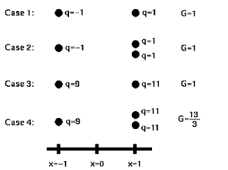
Figure 1: Gradient noise from an irregular particle distribution.

SPH employs a similar procedure to evaluate pressure gradients. The irregular particle distribution gives rise to artificial fluctuations in the local density and pressure with a fractional magnitude of 1, even in a globally uniform fluid. The resulting pressure gradients give rise to Mach 1 fluctuating particle velocities. The physical velocity field may be obtained by spatially averaging. However, for a subsonic situation, a large number of particles must be averaged to yield a smooth flow. Therefore, the resolution per particle is quite low.

SPH correctly captures the physics of fluid turbulence in spite of the loss of resolution from pressure gradient noise, however the inclusion of magnetic fields is inviable. Consider a uniform magnetic field in a stationary fluid. The gradient noise in the induction equation will quickly produce small scale fluctuating fields with the same magnitude as the uniform field. These will give rise to extreme forces and hence even more magnetic fluctuations, resulting in instability.

GPM suppresses noise in the pressure and magnetic gradients, promoting reduced particle velocity fluctuations and enabling the inclusion of magnetic fields. An additional measure may be taken to quell noise in subsonic flows. Here, the physical density fluctuations have a magnitude of $\Delta\rho/\rho\sim M^{2}$, where $M$ is the Mach number. If the density is evaluated from local smoothing, an irregular particle distribution adds fractional density fluctuations of order unity, triggering Mach number unity pressure and velocity fluctuations. This can be corrected by regarding density as a particle property which is evolved according to the continuity equation.

2.2 Gradient Particle Magnetohydrodynamics

The GPM gradient evaluation corrects for the irregular particle distribution. We first consider the 1-D case. Assume that a quantity $q$ has a spatial profile of $q=A_{0}+A_{1}x$ and evaluate the quantities

$$Q_{0}=\sum_{i}qmW=A_{0}\sum_{i}mW+A_{1}\sum_{i}mxW$$ (2)

$$Q_{1}=\sum_{i}qmxW=A_{0}\sum_{i}mxW+A_{1}\sum_{i}mx^{2}W$$ (3)

with the sum occurring over neighboring particles inside the smoothing sphere. The smoothing kernel is $W(r)=exp(-4r^{2}/h^{2})$, where $h$ is the smoothing length and $m$ is the mass of the neighbor particle. If the particles are symmetrically distributed, the $A_{1}$ term in (2) and the $A_{0}$ term in (3) are zero, and

$$A_{0}=\frac{\sum_{i}qmW}{\sum_{i}mW}\hskip 42.67912ptA_{1}=\frac{\sum_{i}qmxW}{\sum_{i}mx^{2}W}$$ (4)

These formulae are equivalent to the SPH evaluation. If the particle distribution is irregular, the $2\times 2$ matrix may be solved to obtain $A_{0}$ and $A_{1}$. For three dimensions, assume $q=A_{0}+A_{1}x_{1}+A_{2}x_{2}+A_{3}x_{3}$ and solve the $4\times 4$ matrix. GPM can be further extended to second order by solving the $10\times 10$ matrix resulting from $q=A_{0}+A_{1}x_{1}+A_{2}x_{2}+A_{3}x_{3}+A_{11}x_{1}^{2}+A_{22}x_{2}^{2}+A_{33}x_{3}^{2}+A_{12}x_{1}x_{2}+A_{13}x_{1}x_{3}+A_{23}x_{2}x_{3}$. Second order allows the viscous and resistive terms to be evaluated directly.

2.2.1 Convergence

GPM quantities can be evaluated to a hierarchy of orders. Consider the calculation of a 1D gradient of $q$ where $q=A_{0}+A_{1}x+A_{11}x^{2}+\cdots$. We have

$$Q_{1}=\sum_{i}qxW=A_{0}\sum_{i}qxW+A_{1}\sum_{i}qx^{2}W+A_{11}\sum_{i}qx^{3}W+\cdot\!\cdot\!\cdot.$$ (5)

The magnitudes of the RHS terms for an irregular particle distribution are $A_{0}hn^{1/2}+A_{1}h^{2}n+A_{11}h^{3}n^{1/2}+\cdots$, where $h$ is the smoothing length and $n$ is the number of particles inside the smoothing sphere. Terms of odd order in $h$ have zero mean, and for them we specify the fluctuating magnitude. Terms of even order in $h$ have a positive mean with the specified magnitude. In the evaluation of $A_{1}$, the $A_{0}$ and $A_{11}$ terms constitute the error. The fractional error due to $A_{0}$, $n^{1/2}A_{0}/(hA_{1})$, is unbounded, necessitating the simultaneous evaluation of $A_{0}$ and $A_{1}$. The fractional error due to $A_{11}$ is $n^{-1/2}hA_{11}/A_{1}$. An imposed viscosity can ensure that $A_{11}h$ is less than the RMS value of $A_{1}$, and so the $A_{11}$ term can be neglected when evaluating $A_{1}$. Similarly, the evaluation of $A_{11}$ requires $A_{0}$ and $A_{1}$ and not $A_{111}$ because a sufficiently smooth profile will have $A_{111}h<A_{11}(RMS)$.

3 Application of GPM to MHD

The GPM algorithm is essentially a recipe for correctly computing gradients in a Lagrangian fluid code. In this section, we describe the application of the GPM algorithm to create a working code for MHD simulation. We first discuss the basic application to the most simple MHD system neglecting viscosity and resistivity, describing the kernel used and the spatial and temporal order of the method. Next we describe the incorporation of viscosity into the code and suggest a method for the elimination of magnetic divergence. Finally, advanced features to improve the method are described.

3.1 Basic Application

The governing equations of MHD are the momentum equation, the induction equation, the continuity equation, and the energy equation:

$$d_{t}v=-\frac{1}{\rho}\nabla P+\frac{1}{4\pi\rho}(\nabla\times b)\times b+\nu\nabla^{2}v$$ (6)

$$d_{t}b=b\cdot\nabla v-b\nabla\cdot v+\eta\nabla^{2}b$$ (7)

$$d_{t}\rho=-\rho\nabla\cdot v$$ (8)

$$d_{t}e=-\frac{P}{\rho}\nabla\cdot v.$$ (9)

The system of MHD equations is closed using the adiabatic equation of state

$$P=(\gamma-1)\rho e.$$ (10)

Quantity	Symbol	Quantity	Symbol
Velocity	$v$	Magnetic field	$b$
Density	$\rho$	Pressure	$P$
Energy density	$e$	Ratio of specific heats	$\gamma$
Viscosity	$\nu$	Resistivity	$\eta$

In all our tests, we have chosen the 3-D adiabatic index for a monatomic gas, $\gamma=5/3$.

We begin with an ideal MHD system, neglecting viscosity and resistivity. To apply the GPM algorithm to the governing equations, it is necessary to choose the form of the kernel $W(\mathbf{r},h)$ and the smoothing radius $h$ over which the kernel applies.

For a test particle at position ${\bf r}$ and a neighbor at position ${\bf r}^{\prime}$, we choose a Gaussian kernel of the form

$$W(\mathbf{r}-\mathbf{r}^{\prime},h)=\frac{1}{N}e^{\frac{-4(\mathbf{r}-\mathbf{r}^{\prime})^{2}}{h^{2}}}$$ (11)

for $\mathbf{r}-\mathbf{r}^{\prime}\leq h$. We cut off the Gaussian at $r=h$, so that for $\mathbf{r}-\mathbf{r}^{\prime}>h$, $W(\mathbf{r}-\mathbf{r}^{\prime},h)=0$. The normalization factor $N$ must be chosen such that the kernel satisfies the normalization condition

$$\int_{-\infty}^{\infty}W(\mathbf{r}-\mathbf{r}^{\prime},h)d\mathbf{r}^{\prime}=1.$$ (12)

For a Gaussian truncated at $r=h$, the normalization factor is thus given by

$$N=h^{3}\pi^{3/2}[\mathrm{Erf}(2)]^{3}.$$ (13)

All particles within a radius $h$ of the test particle will contribute to the MHD forces on the test particle with the weight of each particle’s influence given by smoothing kernel. An appropriate choice of smoothing length $h$ must be made in order to include enough neighbors within the smoothing sphere to yield a good sampling of the local fluid characteristics, and thus calculate gradients accurately. To satisfy this condition, the minimum number of neighbors necessary is approximately 12 neighbors in 2-D simulations and 32 neighbors in 3-D. This estimate is made assuming that particles do lie on a uniform grid and that $h\simeq 2s$, where $s$ is the interparticle separation. In practice, if the particles do become irregularly distributed, a greater number of neighbors should be included in the smoothing sphere to insure that local fluid conditions are sampled adequately.

The order of the GPM method is specified according to the computing resources available and the desired accuracy of the solution. In 3-D, a first order GPM calculation requires the inversion of a $4\times 4$ matrix, and a second order calculation requires a $10\times 10$ matrix to be inverted. We accomplish the inversion using LU Decomposition. It is worthwhile to note that, for each fluid quantity whose gradient is to be calculated— i.e. pressure or a component of velocity—the determination of the lower and upper triangular matrices needs only be done once per particle. Any gradient desired for that particle is calculated by backsubstitution using the same decomposed matrices.

The timestepping employed for these tests was a simple Eulerian first-order scheme.

In order to avoid unphysical fluctuations in the density, the mass density $\rho$ was evolved entirely as a particle characteristic rather than being coupled to the local number density of particles. Hence, our “particles” are really not physical entities at all but simply positions where we know information about the fluid. This simplifies the setting of initial conditions and also allows the resolution to be enhanced in a particular region by simply placing more particles in that region. This freedom is useful because you do not a priori desire less resolution in a region which has a lower density. It does, however, allow for the mass density to move with respect to the particle points in our simulation. If this causes difficulties to arise, they can be alleviated by particle removal and replacement as will be discussed in Section 3.4.

The basic implementation of GPM for MHD as described thus far was susceptible to a slowly growing smoothing length related instability. Hence, the addition of viscosity was found to be necessary to yield a stable scheme.

3.2 Viscosity

Lagrangian codes typically have a very small diffusivity when compared to grid-based methods for the same problem. We have found that GPM, since it removes a significant component of noise present in SPH codes, is even more non-dissipative. The addition of artificial velocity was found necessary to stabilize a slowly growing smoothing length related instability and to prevent particle interpenetration in the presence of shocks. We investigated the different forms of artificial viscosity and also explored the possibility of using real viscosity and resistivity in the case of second order GPM when the Laplacian of velocity ${\bf v}$ and magnetic field ${\bf b}$ can be calculated directly.

3.2.1 Artificial Viscosity in GPM

A common treatment of artificial viscosity in finite difference calculations involves the addition of a bulk viscosity, which enhances the pressure when $\nabla\cdot\mathbf{v}<0$ (Roache, 1975). In the momentum equation, the pressure $P$ is replaced by $P+q$, where

$$q=\left\{\begin{array}[]{ll}-\alpha\rho hc_{s}\nabla\cdot\mathbf{v}+\beta\rho h^{2}(\nabla\cdot\mathbf{v})^{2}&\mbox{if $\nabla\cdot\mathbf{v}<0$}\\ 0&\mbox{if $\nabla\cdot\mathbf{v}>0$}.\end{array}\right.$$ (14)

Here $\alpha$ and $\beta$ are dimensionless constants, $h$ is the cell width, $\rho$ is the local density, and $c_{s}$ is the local sound speed.

Monaghan and Gingold (1983) suggested that for SPH, which is significantly less diffusive than grid-based methods, artificial viscosity is always necessary but that the above formulation smears out shock fronts excessively because $\nabla\cdot\mathbf{v}$ is averaged over all particles in a smoothing radius. They found a more effective artificial viscosity based on interparticle velocity differences (Monaghan, 1985, 1992).

We have used a similar approach to Monaghan (1992), estimating $\nabla\cdot\mathbf{v}$ by the velocity differences between particles and enhancing the pressure of approaching particles by $q$ as in equation (14). In one-dimension, we estimate by Taylor expansion the velocity divergence between a test particle $i$ and its neighbor particle $j$ as

$$\frac{(v_{xi}-v_{xj})(x_{i}-x_{j})}{(x_{i}-x_{j})^{2}}\simeq\frac{1}{x_{i}-x_{j}}\left\{v_{xi}-\left[v_{xi}+(x_{j}-x_{i})\left.\frac{\partial v_{x}}{\partial x}\right|_{x_{i}}+\cdots\right]\right\}\simeq\frac{\partial v_{x}}{\partial x}.$$ (15)

In practice, we approximate the 3-dimensional interparticle divergence as

$$\nabla\cdot\mathbf{v}\simeq\frac{(\mathbf{v}_{i}-\mathbf{v}_{j})\cdot(\mathbf{x}_{i}-\mathbf{x}_{j})}{(\mathbf{x}_{i}-\mathbf{x}_{j})^{2}+(\epsilon h)^{2}/4}$$ (16)

where $\epsilon=0.1$ and $h$ is the GPM smoothing radius. The extra term in the denominator prevents the singularity as $\mathbf{x}_{i}-\mathbf{x}_{j}\rightarrow 0$. The modified pressure $P+q$ is given by equation (14) with $\nabla\cdot\mathbf{v}$ estimated by equation (16). Thus, the pressure from each neighboring particle is enhanced by the viscous term only when it is approaching the test particle. The modified pressure $P+q$ is then used in the standard GPM implementation to find the gradient of the pressure in the momentum equation

$$d_{t}\mathbf{v}=-\frac{1}{\rho}\nabla(P+q)+\frac{1}{4\pi\rho}(\nabla\times\mathbf{b})\times\mathbf{b}.$$ (17)

The artificial viscosity of the form in equation (14) behaves as a normal bulk viscosity plus a von Neumann-Richtmeyer bulk viscosity. For linear problems in which the stabilizing effects of an artificial viscosity are desired, but the dissipation is to be kept to a minimum, values of $\alpha=0.05$ and $\beta=0.1$ have proved sufficient to stabilize smoothing length related computational instabilities but have not altered the waveform. For shock capturing, larger values of $\alpha=0.5$ and $\beta=1.0$ can prevent particle interpenetration and damp post-shock oscillations.

3.2.2 Real Viscosity and Magnetic Diffusivity

The ability for second order GPM to yield not only the gradient but also the second derivative of fluid quantities opened up the potential for employing a real viscosity and real resistivity in simulations. Initial tests with real viscosity, however, have demonstrated a slowly growing instability which prevented long-time simulations from being run.

3.3 Magnetic Divergence

GPM does not preserve magnetic divergencelessness, however divergences can be removed with a procedure analogous to a gravitational potential solution. Solve $\nabla^{2}\Phi=-\nabla{\bf b}$ for $\Phi$ and reset the magnetic field to ${\bf b}_{\mathrm{new}}\leftarrow{\bf b}_{\mathrm{old}}+\nabla\Phi$. The solution of Laplace’s equation may be piggy-backed with the $N\log_{2}N$ tree gravitation algorithm.

3.4 Advanced Features

The most simple advanced feature that has been implemented with the GPM is a variable smoothing length $h$. By adjusting the smoothing length to encompass a specified number of nearest neighbors, we can tackle a problem involving multiple density scales without excessive smoothing in high density regions or undersampling of nearest neighbors in the low density regions. In practice,we choose an optimal number of neighbors, i.e. 45 neighbors for a 3-D calculation, and allow a range of $\pm 33\%$ from that number. We have implemented this featuring for testing and have noted in Section 4 when a variable smoothing length has been used for a test run.

Because the mass density $\rho$ is not fixed to the “particle” points, it is possible over many timesteps for the mass to slip with respect to the particles. Two possible problems can result: two particles may move very close together and effectively reduce the resolution of the simulation by including a virtually redundant point, or particles may move away from each other leaving a region of the fluid that is poorly sampled. Particle removal and replacement can solve this problem. Particle removal has been implemented and has proven useful in the case of collapse in a fixed central gravitational potential. When two particle are separated by a distance of $r<h/100$, one particle is removed and the fluid quantities (including position) are combined to conserve mass, center of mass, momentum, energy, and magnetic flux. Particle replacement in poorly sampled regions has not yet been implemented.

The simulation of a galactic disk with magnetic fields presents severe obstacles to any numerical technique. Turbulent structure exists at widely varying space and time scales, rotation times vary widely with radius, and magnetic fields and gravity are significant. For example, molecular cloud and supernova dynamics occur at substantially smaller scales than that of the disk. Also, the ISM consists of a mixture of phases with widely varying temperature and density. For a grid-based code, the timestep is determined by the fastest and smallest scales in the system. If these scales occupy a small fraction of the volume, the timestep is too small for the majority of the system. A cylindrical coordinate system co-rotating with the inner radii can in part compensate for the range of radial dynamics, but it cannot simultaneously offer high resolution anywhere but at the inner radii.

We plan to incorporate the particle-based GPM fluid algorithm with a Barns-Hut tree to efficiently handle situations with widely varying space and time scales. In this code, particles have independent timesteps and smoothing lengths which adjust to local conditions. Timesteps are Lagrangian, as opposed to Eulerian, which means they are a function of local velocity dispersion, as opposed to the global sweeping velocity. Gravitational forces and near-neighbor lists for GPM are computed simultaneously with a Barnes-Hut tree, an $N\log_{2}N$ operation. The tree is rebuilt once every 16 timesteps, and this operation constitutes a negligible fraction of the computational time. The program is MPI parallel, with communication occurring between nodes only at the start of a tree rebuild. Memory access is not a factor in execution speed, which is accomplished by organizing the data by particle, linear in memory. Nearby particles in space are stored nearby in memory to minimize cache misses. Finally, data is prefetched from RAM in advance of use, with the prefetch occuring simultaneously with other floating point operations.

4 Validation

In this section, we present the results of a suite of validation tests to determine the performance of the GPM algorithm in simulating MHD phenomena. We tested the propagation of linear and nonlinear sound waves and determined a dispersion relation for varying spatial resolution. Sound wave test results are compared with SPH results using the publicly available Hydra code by Couchman et. al. (1995). Slow, Alfvén , and fast MHD waves were tested at the full range of angles between the direction of propagation ${\bf k}$ and the magnetic field ${\bf b}$. A polar plot of MHD wave velocities shows excellent agreement with theory at moderate resolution. An advective MHD test is performed by initializing a magnetized vortex and following the evolution of the particles and the magnetic field; good agreement was found with results from a spectral MHD code by Maron and Goldreich (2001). The standard Sod shock test (Sod, 1978) was performed to determine the shock-capturing ability of GPM. Finally, a 3-D collapse problem was run to demonstrate the multiscale capability of GPM using variable smoothing lengths.

All tests were run with a minimum of two dimensions, since a lot of the problems that arise using SPH disappear when it is run in only one dimension; in all cases, no differences were seen between two-dimensional and three-dimensional GPM simulations when run with the same parameters and initial conditions. In all plots shown here, all redundant points are plotted to demonstrate the minimal cross-field dispersion characteristic of GPM. All tests were run using the adiabatic index appropriate for 3-D gas dynamics, $\gamma=5/3$.

Clearly additional refinement of the GPM method is possible, but these tests demonstrate the validity of the method in simulating subsonic and supersonic flows with magnetic fields over varying spatial scales.

4.1 Sound Waves

To test the ability of GPM to handle hydrodynamics accurately, we performed tests with linear and nonlinear sound waves and determined the dispersion relation of the method when the resolution is varied.

Figure 2 shows the second-order GPM result for the propagation of a linear acoustic wave with a sinusoidal profile. Particles were placed on a regular grid in a periodic box of size $1.0\times 0.125\times 0.015625$ using $64\times 8\times 1$ particles. The initial conditions for a single eigenmode moving to the right were imposed with a velocity perturbation of $\delta v=0.1\%$. The smoothing length was fixed at $h=0.0488496$ and the CFL fraction was $0.0125$ using the loose CFL condition. Artificial viscosity was employed with $\alpha=0.05$ and $\beta=0.1$. The sound speed is $c_{s}=1.0$, so the wave should repeat itself each $1.0$ time units; the plot time is $t=10.0$.

Figure 2: Second-order $64\times 8\times 1$ GPM result for the propagation of a right-moving linear sound wave with amplitude $\delta v=0.1\%$ at time $t=10.0$. The analytical result is the solid line and the boxes indicate the GPM results with a connecting line to assist in comparison.

The discrepancy with respect to the analytical expectation can be divided into amplitude and phase error: the amplitude error appears to be related to the timestep used and the value of artificial viscosity employed, and the phase error (error in wave propagation speed) is reduced with increasing spatial resolution.

Figure 3 presents the dispersion relation for linear sound waves for varying wavenumber (or equivalently for varying number of particles per wavelength). All parameters are the same as the previous test expect for: variable smoothing length is employed using approximately 16 neighbors per particle ($\pm 33\%$); the CFL fraction is $0.025$; and the resolution, or number of particles per wavelength, is varied as indicated with corresponding changes in the box size.

Figure 3: Dispersion relation for linear sound wave using the GPM algorithm.

The figure shows that for 32 or more particles per wavelength the GPM results agree well with analytical predictions.

The steepening of a nonlinear sound wave into a shock is a sensitive test of any hydrodynamical scheme. Figure 4 shows the GPM nonlinear sound wave compared to an inviscid method of characteristics solution.

Figure 4: The propagation and steepening of a nonlinear sound wave of amplitude $\delta v=5.0\%$ using first order GPM with $64\times 8\times 1$ particles. The analytical solution from an inviscid method of characteristics is given by the solid line and the boxed line shows the GPM results. The analytical solution forms a shock at $t=1.74$.

The parameters for this simulation are the same as the linear sound wave above expect for: the amplitude of the perturbation is $\delta v=5.0\%$, a variable smoothing length with approximately 16 neighbors is used, and the calculation is done using first order GPM. Analytically the formation of a shock occurs at $t=1.74$. The GPM results are plotted with analytical solutions for $t=1.0$ and $t=1.7$. Because the artificial viscosity is quite low ($\alpha=0.05$, $\beta=0.1$), this simulation is susceptible to large post-shock oscillations; the beginnings of a post shock oscillation can be seen in the GPM result at $t=1.7$.

Figure 5 compares GPM results for a linear sound wave with results from the SPH code Hydra (Couchman et. al., 1995). The SPH code used $32\times 32\times 32$ particles on a regular lattice in a periodic box of size $1.0\times 1.0\times 1.0$. Hydra is a publicly available SPH code used primarily for cosmological simulations, so we choose to turn off as many of the advanced options as possible: gravity, expansion, and cooling were shut off. The sound speed was set to $c_{s}=1.0$ and a variable smoothing length is used with 32 neighbors specified. We used a simple but rigorous nearest neighbor search for GPM which employs of order $N^{2}$ computations so, due to computational limitations, the first-order GPM calculations used $32\times 8\times 8$ particles on a regular lattice in a periodic box of size $1.0\times 0.25\times 0.25$. Artificial viscosity was turned off, the sound speed was $c_{s}=1.0$, variable smoothing lengths were used with 32 neighbors, and the CFL fraction was $0.025$ according to the initial particle separation. Both codes were initialized with a single sound wave propagating in the $x$ direction with amplitude $\delta v=0.1\%$. The results are compared at $t=1.0$ and for both codes all particles are plotted.

Figure 5: GPM vs. SPH results for a linear sound wave of amplitude $\delta v=0.1\%$. All SPH particles, which show a tremendous amount of dispersion, are plotted as small dots and the average of all redundant particles is shown as a circle. The GPM particles are plotted as boxes and show no dispersion. The analytical result is the solid sinusoidal line.

Note that after one sound crossing time of the box, the individual SPH particles have suffered a tremendous amount of cross-field dispersion. This is a result of the substantial unphysical noise inherent in the SPH scheme due to its Monte Carlo nature; only an average of many particles will provide an accurate result. GPM demonstrates no unphysical dispersion.

GPM results for a nonlinear sound wave of amplitude $\delta v=5.0\%$ are compared to SPH results in Figure 6. All parameters are the same as for the previous comparison except: the number of neighbors for GPM variable smoothing length was 45; and, for SPH, $32^{3}$ particles are placed randomly in the box and, for GPM, $32\times 8\times 8$ particles are placed randomly.

Figure 6: GPM vs. SPH results for a nonlinear sound wave of amplitude $\delta v=5.0\%$. Again, all particles for both methods are plotted; demonstrating the large dispersion of SPH and small dispersion of GPM. Bin averages of width $\Delta x=0.01$ for SPH results are given by circles.

Again, the large dispersion of SPH particles is clearly seen; only averages of many particles, taken over all particles within bins of width $\Delta x=0.01$, provide a solution that resembles the analytical result. GPM shows no dispersion and hence requires no averaging to yield an accurate solution; this encouraging result suggests that the effective resolution of GPM is significantly higher than that of SPH because there is no need to average over a large number of particles to eliminate unphysical noise and obtain accurate results.

4.2 MHD Waves

To test the ability of the GPM algorithm to accurately simulate MHD phenomena, simulations of slow, Alfvén , and fast MHD waves were performed over the full range of angles between the wave propagation direction ${\bf k}$ and the direction of the unperturbed magnetic field ${\bf b}$. A complete discussion of their phase speeds and mode eigenvectors is given in Appendix C. The results of these tests are easily summarized on a polar plot of MHD linear wave propagation as shown in Figure 7. In this plot, the direction of the magnetic field is along the ordinate and the angle between the magnetic field ${\bf b}$ and the wave propagation direction ${\bf k}$ is the polar angle from the ordinate to the abscissa. The radius of the polar coordinate corresponds to the magnitude of the wave velocity. The analytical solutions are plotted as solid lines and the boxes represent values obtained by the GPM code. The second order GPM simulations were run with $32\times 5\times 5$ particles on a uniform lattice in a periodic box of size $1.0\times 0.15625\times 0.15625$. The smoothing length was fixed at $h=0.0508$ and artificial viscosity parameters of $\alpha=0.05$ and $\beta=0.1$ were applied. The sound speed was $c_{s}=1.0$, the Alfvén speed was $v_{A}=2.0$, and the angles between ${\bf b}$ and ${\bf k}$ were $0^{o}$, $15^{o}$,$30^{o}$, $45^{o}$,$60^{o}$, $75^{o}$, and $90^{o}$. The CFL fraction was $0.0125$ using the loose CFL constraint. A single eigenmode for each of the three wave types was used with the amplitude of the velocity perturbation $\delta\mathbf{v}\cdot\hat{\mathbf{k}}=0.1\%$; the direction of propagation is along the $x$-axis for all simulations.

Figure 7: Polar plot of the MHD wave speeds vs. the angle between the magnetic field ${\bf b}$ and the wave propagation direction ${\bf k}$. The analytical solutions for slow, Alfvén , and fast MHD waves are indicated by the solid lines; second order GPM results for $32\times 5\times 5$ simulations are given by the boxes.

The GPM algorithm gives an excellent agreement with theory for all three MHD waves over the entire range of propagation directions.

Examples of several of the simulations summarized in Figure 7 are shown in Figures 8 and 9. A slow MHD wave and a fast MHD wave both propagating at $\theta=45^{o}$ from the magnetic field are shown in Figure 8 for the third repetition time in the periodic box (corresponding to $t=4.53$ for the slow wave and $t=1.40$ for the fast wave).

Figure 8: Slow MHD wave (left) and fast MHD wave (right) propagating at $\theta=45^{o}$ from the magnetic field. Plots are shown at three crossing times of the periodic box for that wave mode, $t=4.53$ for the slow wave and $t=1.40$ for the fast wave. Analytical results are given by the solid line and second order GPM results with $32\times 5\times 5$ particles are given by the boxed line.

Figure 9 shows a shear Alfvén wave propagating at $\theta=0^{o}$ and a magnetoacoustic wave (fast wave at $\theta=90^{o}$); both are plotted for the third repetition in the periodic box, corresponding to $t=1.5$ and $t=1.342$, respectively.

Figure 9: Shear Alfvén wave propagating parallel to the magnetic field (left) and a magnetoacoustic wave propagating transverse to the magnetic field (right). Plots are shown at three crossing times of the periodic box for that wave mode, $t=1.5$ for the shear Alfvén wave and $t=1.342$ for the magnetoacoustic wave. Analytical results are given by the solid line and second order GPM results with $32\times 5\times 5$ particles are given by the boxed line.

4.3 Advective MHD Problem: 2-D Magnetized Vortex

To test the GPM evolution of a dynamical magnetic field, we simulated a 2-D vortex flow superimposed with an initially uniform magnetic field. The flow is initialized with an azimuthal flow profile of the form

$$v_{\phi}=v_{0}\frac{r}{r_{0}}e^{(1-r^{2}/r_{0}^{2})}$$ (18)

with the values $v_{0}=0.1$ and $r_{0}=0.1667$ in a 2-D periodic box of size $1.0\times 1.0$. The initial weak magnetic field is ${\bf b}=0.001\hat{\mathbf{x}}$. Second order GPM is used with a fixed smoothing length $h=0.123$ and artificial viscosity parameters $\alpha=0.05$ and $\beta=0.1$. The $32^{2}$ points are placed on a pseudorandom grid and the CFL fraction is $0.0125$ assuming all particles are separated by a distance $s=0.03125$. The sound speed $c_{s}=1.0$. The radius at the peak of the azimuthal velocity will have undergone one full rotation in a time $t=10.47$. Figure 10 shows the GPM results at time $t=10.0$.

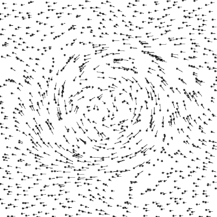
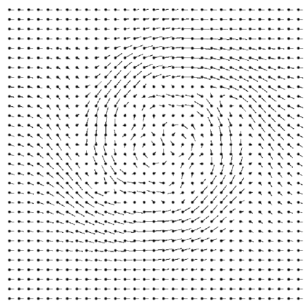
Figure 10: GPM (left) and spectral MHD (right) simulation results 2-D magnetized vortex. The spheres represent particle positions and the arrows represent magnetic fields. A spectral code does not have particles, and so the particles shown here serve only as markers for the magnetic field arrows.

For comparison, we also simulated the vortex with a spectral MHD code (Maron and Goldreich, 2001) and found good agreement with the GPM result. For the GPM calculation, the magnetic field evolution is stable and magnetic structures are resolved to 2 interparticle radii. In fact, the effective viscosity of GPM is almost as good as that of the spectral simulation.

In a purely hydrodynamic version of this simulation using SPH, which is not shown, the vortex stops turning after roughly one quarter rotation due to intrinsic diffusivity of the SPH method. The GPM vortex has not slowed appreciably.

4.4 Shocks

To test the shock-capturing capabilities of GPM, we used the standard Sod (1978) 1-D shock test. Although quantities vary only in one dimension, these tests were conducted in more than one dimension to insure that there is no unphysical cross-field dispersion into the redundant dimensions. This stringent test begins with an initial pressure and density discontinuity at an interface; compression and rarefaction waves propagate into either side of the interface with a contact discontinuity visible in the density and energy profiles only. We choose the same initial conditions as the Sod (1978) paper: $p=1.0$ and $\rho=1.0$ to the left of the discontinuity, $p=0.1$ and $\rho=0.125$ to the right, and zero velocity everywhere. And, for this problem only, we employ the adiabatic index $\gamma=1.4$ to retain consistency with the original paper. The resulting profiles for density, pressure, energy, and $x$-component of the velocity are shown in Figure 11 for time $t=0.3$.

Figure 11: The profile results of the standard Sod (1978) 1-D shock test for density (upper left), pressure (upper right), energy (lower left), and $x$-component of velocity (lower right) for the time $t=0.3$. Note the contact discontinuity visible in the density and $x$ velocity profiles.

4.5 Collapse Problem

To test the multiscale capability of the GPM code, we choose to do a 3-D collapse problem in a fixed gravitational potential and demonstrate the attainment of a state of hydrostatic equilibrium.

5 Discussion

The validation tests which have been presented here have all been performed using a first-order Eulerian time stepping scheme. To achieve computational stability, we observed the timestep constraint to be very tight: in most cases, the fraction of the Courant-Friedrichs-Lewy limit was $0.0125$ to prevent any growth in the amplitude of a linear wave. A value of $0.025$ was also used and, although the amplitude was seen to grow slightly (a few percent) over a very long time ( around 100 sound crossing times of the periodic box), it did not cause any problems. A higher-order time stepping scheme may help this significantly, but a tighter timestep constraint may not be a problem if the GPM algorithm proves to have far superior spatial resolution compared to SPH.

In the comparisons presented above with SPH results, GPM appears to be able to resolve more detail with an equivalent number of particles than SPH. Because SPH is a Monte Carlo method, the error in the value of a fluid quantity at any point scales as $N^{-1/2}$ for a random distribution of particles and as $N^{-1}$ for a pseudo-random distribution. Therefore, to resolve the quantity to high precision, a number of points must be averaged. But GPM gives the value of the fluid quantity at each point to the error of the chosen order of the method, so there is no need for an averaging. The spatial averaging of any quantity necessarily involves a reduction in the effective resolution of the method. Thus,a GPM simulation may indeed demonstrate a significant gain in resolution over a simulation in SPH with an equivalent number of particles. And, GPM is capable of stably handling MHD, while SPH must resort to various tweaks of the method to model MHD effects.

Another advantage of GPM over SPH, which cannot be extended beyond a first-order scheme, is that GPM can, in theory, determine fluid profiles to a specified polynomial degree. In practice, the limitations of computational power may prevent use of the method beyond second order. A first-order calculation requires the inversion of a $4\times 4$ matrix, a second-order a $10\times 10$ matrix, a third oder calculation a $20\times 20$ matrix, and so on. Hence, a third-order calculation is likely to be too computationally expensive to justify the higher-order determination. But, even if one only utilizes first-order GPM, it is useful to have a higher-order extension of the method for convergence tests.

In the application of GPM presented here, we do not couple the mass density of the fluid with the number density of “particles” used in the calculation. Hence, GPM is not a particle method in the traditional sense; it behaves more like a deforming mesh of points at which we know information about the fluid. This prevents large unphysical fluctuations in the density and allows the method to be extended to higher order. It also simplifies the setting of initial conditions in that the number density of points does not have to be proportional to the local mass density. As well, resolution can be enhanced in a region of interest by simply placing more particles there without disturbing the behavior of the fluid. The disadvantage of doing this is that it is possible, over long periods of time, for mass density to slip away from the particles; conversely, it is possible for the particles to gather in some areas, leaving voids in other areas where the fluid properties are undersampled. A method of particle removal where an excess of particles have gathered and particle replacement where voids leave the fluid undersampled can rectify this potential problem. In the simulations presented here, we did not find any problems of this nature.

The other disadvantage of Lagrangian methods in general is the difficulty of ensuring strict conservation of quantities such as mass, linear and angular momentum, energy, and magnetic flux. Further tests of GPM will need to be carried out to determine the conservation properties of GPM and the magnitude of any errors that arise.

Because GPM is very non-dissipative, discontinuities established in initial conditions must be smoothed before beginning the simulation. This is accomplished by using a first-order GPM calculation, either with fixed or variable smoothing length, to determine the average $\overline{q}$ of a fluid quantity $q$ and finding the smoothed value $q_{sm}$ using $q_{sm}=q+f_{sm}(\overline{q}-q)$. In practice, one desires a smoothing length large enough so that a shock discontinuity is spread out over at least $4$ particles.

When performing a simulation with an external potential, as in the 3-D collapse problem above, we found that it is critical for the form of the applied force to be well sampled by particles. If this is not ensured, then the GPM algorithm cannot balance the applied external forces with the internal fluid forces. It is wise, also to smooth out the gravitational force so as not to have any harsh discontinuities in its form. We found that a smoothed external gravitational force of the form

$$F_{g}(r)=-\frac{GM}{r^{2}}\left(1-e^{-(r/r_{0})^{3}}\right)\hat{\mathbf{r}}$$ (19)

worked very well.

Finally, when doing isolated problems, we consider the question of the ability of GPM to correctly determine forces at boundaries. If there are enough particles within the smoothing sphere, GPM seems to do a reasonably good job of determining the forces. In practice, it seems best that the gradient goes to zero at the boundaries so that all forces will go to zero. Thus, it is a good idea to place particles far enough out that the forces are indeed nearly zero. Since the mass density is not related to particle number density, this can be done with a very sparse distribution of particles.

6 Conclusion

The past two decades have seen extensive use of Lagrangian numerical methods to model astrophysical phenomena. SPH has proven to be an invaluable tool for astrophysics to tackle problems with other numerical methods simply could not handle. But, as we move into the next decade, an improvement in the precision of methods is needed to refine existing theoretical models and to investigate problems in new regimes. In the absence of a viable extension of SPH to include magnetic effects, astrophysicists have turned to grid-based methods employing AMR to study MHD problems with large density contrasts. In this environment, we present Gradient Particle Magentohydrodynamics (GPM) as an alternate Lagrangian method which accurately and stably simulates MHD phenomena and which potentially can yield a significant improvement in spatial resolution over SPH. Various algorithms employed in astrophysical computation are compared in Appendix A.

The simple recipe for the GPM algorithm is presented here and its application to develop an MHD simulation code is described. The GPM scheme can be extended to higher orders and is observed to be very non-diffusive. We have inclusion validation tests to show the behavior of GPM in modeling linear and nonlinear sound waves, the full suite of MHD waves, an advective MHD problem, shocks, and three-dimensional collapse. These tests demonstrate clearly the promise of this technique, although there is certainly room for refinement of the method.

Although the two schemes are quite closely related in spirit, we believe GPM to be superior to the SPH scheme for computing fluid forces. The similarity of the two numerical methods—that both simply need a list of the nearest neighbors and the values of the fluid quantities at those particles—makes the implementation of GPM highly attractive. Any existing high performance SPH code could easily be modified to employ the GPM algorithm as the heart for the determination of MHD forces instead of the SPH formulation.

Currently, the development of AMR for grid-based techniques is extending the capability of grid-based codes into the regime heretofore dominated by Lagrangian codes. But, for the computational power available today, AMR is still limited to a small number of grid-refinement steps (in the neighborhood of 5 to 10 levels of refinement). As well, grid-based codes are susceptible to upwinding and transport diffusion, and those incorporating AMR even more so. A Lagrangian code based on GPM is an ideal complement to the computational effort of AMR codes. The strengths of Lagrangian codes are the weaknesses of grid codes, and vice-versa. But, as computational power increases, both numerical techniques should converge to the same solution from different regimes: AMR from the high-precision, more diffusive side with a smaller resolved range of densities, and GPM from the low-precision, less diffusive side with a greater resolved range of density.

Appendix A Comparison of algorithms

There are 5 major classes of hydro/MHD algorithms, each having strengths and weaknesses. A spectral code computes gradients in Fourier space with the use of the Fast Fourier Transform (Borue & Orszag 1996, Maron & Goldreich 2001). A grid code computes mass and momentum fluxes through grid-cell boundaries. An example is the 3D Compressible MHD code “Zeus”, a well validated program (Stone & Norman, 1992 I, 1992 II) enjoying widespread use in the astrophysical community. An adaptive grid (Berger & Oliger 1984, Berger & Colella 1989) additionally allows cells to be dynamically subdivided in areas of need. SPH (Monaghan 1992, Couchman, et. al., 1995) is smoothed particle hydrodynamics and GPM is gradient particle magnetohydrodynamics.

Table 1: The principal fluid dynamics algorithms. Items 1-4 refer to physics capabilities of the algorithms. Items 6-9 refer to matters of computational efficiency.

Characteristic	Spectral	Grid	Adaptive grid	SPH	GPM
1) Subsonic	Yes	Yes	Yes	Noisy	Yes
2) Supersonic (Shocks)	No	Yes	Yes	Yes	Yes
3) Magnetic fields	Yes	Yes	Yes	No	Yes
4) Resolution	Best	Good	Good	Poor	Good
5) Code complexity	Easy	Easy	Hard	Easy	Easy
6) Lagrangian timesteps	No	No	No	Yes	Yes
7) Spatial refinement	No	No	Yes	Yes	Yes
8) Variable timesteps	No	No	Yes	Yes	Yes
9) Parallelizable	Yes	Yes	Yes	Yes	Yes

Table 2: Computational efficiency

Subsonic:	The velocities are less than the sound speed.
Supersonic:	The velocities exceed the sound speed, producing
	strong density contrasts and shocks.
Magnetic fields:	The ability to include magnetic fields.
Resolution:	The effective resolution per computational element.
	This property is distinct from spatial refinement.
Code complexity:	The algorithmic complexity of the code.
Lagrangian timesteps:	Timesteps are determined by local velocity
	fluctuations instead of the local average velocity.
	Therefore, larger timesteps can be used, increasing
	computational efficiency.
Spatial refinement:	The ability to focus resolution on areas of interest.
Variable timesteps:	The ability to use smaller timesteps in areas of need
	while the rest of the system can simultaneously evolve
	with a larger timestep.
Parallelizable:	The ability to run on several processors
	simultaneously, increasing execution speed.

Appendix B SPH

SPH simulations serve as a reference for several of our validation tests. Standard SPH is discussed in the ARAA review by Monaghan and has seen extensive refinement since. It is based on the smoothed spatial average, here for a general quantity $q$, of the form:

$$q=h^{-3}\sum_{b}\frac{m_{b}q_{b}}{\rho_{b}}W(r).$$ (B1)

where the subscript $b$ denotes neighboring particles. $W(r)$ is a symmetric smoothing kernel with a characteristic radius $h$, and $\nabla W(r)$ is the gradient kernel. If $q$ is the density, then

$$\rho=h^{-3}\sum_{b}m_{b}W(r).$$ (B2)

The pressure operator is symmetrized to conserve momentum. The subscript $a$ refers to the test particle.

$$-\frac{1}{\rho}\nabla P=-\nabla\frac{P}{\rho}-\frac{P}{\rho^{2}}\nabla\rho=-h^{-3}\sum_{b}m_{b}\left(\frac{P_{b}}{\rho_{b}^{2}}+\frac{P_{a}}{\rho_{a}^{2}}+\Pi\right)\nabla W$$ (B3)

An artificial viscosity has been added through an extra pressure term $\Pi$ that acts only between converging particles.

$$\Pi=\frac{-\alpha c_{ab}\mu_{ab}+\beta\mu_{ab}^{2}}{\rho_{ab}};\hskip 8.5359ptv\cdot r<0\hskip 42.67912pt\Pi=0;\hskip 8.5359ptv\cdot r>0$$ (B4)

$$\rho_{ab}=\frac{\rho_{a}+\rho_{b}}{2}\hskip 42.67912ptc_{ab}=\frac{1}{2}\left(\frac{\gamma_{a}P_{a}}{\rho_{a}}+\frac{\gamma_{b}P_{b}}{\rho_{b}}\right)\hskip 42.67912pt\mu_{ab}=\frac{h(v_{b}-v_{a})\cdot r}{r^{2}+.01h^{2}}$$ (B5)

The density and energy equations have similar forms.

$$d_{t}\rho=-\rho\nabla\cdot v=h^{-3}\sum_{b}m_{b}(v_{a}-v_{b})\cdot\nabla_{a}W$$ (B6)

$$d_{t}e=-\frac{P}{\rho}\nabla\cdot v=\frac{1}{2}h^{-3}\sum_{b}m_{b}\left(\frac{P_{b}}{\rho_{b}^{2}}+\frac{P_{a}}{\rho_{a}^{2}}\right)(v_{a}-v_{b})\cdot\nabla_{a}W$$ (B7)

Appendix C MHD waves

We summarize here the MHD eigenvectors for arbitrary Alfvén and acoustic speeds $v_{A}$ and $v_{S}$ (Shu 1992), assuming only that the fluctuations are small with respect to the Alfvén and acoustic speeds. The uniform magnetic component has a value of $b_{0}$ oriented along $\hat{{\bf z}}$. Define mean and fluctuating quantities as

$$b=b_{0}\hat{{\bf z}}+b_{0}(b_{\hat{a}}\hat{{\bf a}}+b_{\hat{s}}\hat{{\bf s}})\hskip 2.84526pte^{i({\bf k}\cdot{\bf x}-\omega t)}\hskip 22.76219ptv=(v_{\hat{k}}\hat{{\bf k}}+v_{\hat{a}}\hat{{\bf a}}+v_{\hat{s}}\hat{{\bf s}})\hskip 2.84526pte^{i({\bf k}\cdot{\bf x}-\omega t)}$$

$$\rho=\rho_{0}+\rho_{0}\rho_{1}\hskip 2.84526pte^{i({\bf k}\cdot{\bf x}-\omega t)}\hskip 14.22636pt$$

where the unit right-hand polarization vectors $\hat{{\bf k}}$, $\hat{{\bf s}}$, and $\hat{{\bf a}}$ are defined by

$$\hat{\bf a}\equiv{\hat{{\bf k}}\times\hat{{\bf z}}\over[1-(\hat{{\bf k}}\cdot\hat{{\bf z}})^{2}]^{1/2}},\hskip 34.1433pt\hat{\bf s}\equiv{\hat{{\bf z}}-(\hat{{\bf k}}\cdot\hat{{\bf z}})\hat{{\bf k}}\over[1-(\hat{{\bf k}}\cdot\hat{{\bf z}})^{2}]^{1/2}}.$$ (C1)

and $\cos\theta=\hat{{\bf k}}\cdot\hat{{\bf z}}$.

The Alfvén wave dispersion relation is $\omega^{2}/k^{2}=v_{A}^{2}(\hat{{\bf z}}\cdot\hat{{\bf k}})$, and the eigenvectors are

$$\rho_{1}:v_{\hat{a}}:b_{\hat{a}}\hskip 2.84526pt=\hskip 2.84526pt0:\pm v_{A}:-1.$$

The dispersion relations for the fast (+) and slow (-) modes are

$$\frac{w^{2}}{k^{2}}=\frac{1}{2}\left[(v_{A}^{2}+v_{S}^{2})\pm[(v_{A}^{2}+v_{S}^{2})^{2}-4v_{A}^{2}v_{S}^{2}\cos^{2}\theta]^{1/2}\right]$$

The eigenvectors are $\rho_{1}:v_{\hat{k}}:v_{\hat{s}}:b_{\hat{s}}$

$$=\hskip 2.84526pt\cos\psi\sin\psi:\frac{w}{k}\cos\psi\sin\psi:\frac{w}{k}\left[\sin^{2}\psi+\frac{v_{S}^{2}-w^{2}/k^{2}}{v_{A}^{2}}\right]:-\frac{v_{S}^{2}-w^{2}/k^{2}}{v_{A}^{2}}\cos\psi.$$

Acoustic waves are a special case where there is no magnetic field. The progate at the acoustic speed and have an eigenvector of $\rho_{1}:v_{\hat{k}}=1:v_{S}$.

GPM accurately reproduces the wave speeds and eigenvectors for all three polarizations of linear waves for all propagation directions.

Appendix D Application of Courant-Friedrichs-Lewy Timestep Constraint

There are two basic implementation of the CFL time control, loose and strict. Consider the Courant-Friedrichs-Lewy stability criterion that

$$\frac{|v|\Delta t}{\Delta x}\leq 1.$$

We can determine the timestep to use by

$$\Delta t=f_{CFL}\frac{\Delta x}{|v|}$$

where $f_{CFL}$ is the Courant fraction applied to the problem.

The loose implementation finds the mean nearest neighbor particle separation $\overline{s}$ and the standard deviation of that value $\sigma_{s}$. It employs the value $\Delta x=\overline{s}-\sigma_{s}$ and $|v|=\mathrm{max}(v_{f},v_{i(max)})$ where $v_{f}$ is the fast wave speed and $v_{i(max)}$ is the fastest particle speed in the system.

The strict implementation calculates the value $\frac{\Delta x}{|v|}$ for each particle and its nearest neighbor where $\Delta x$ is the distance to the nearest neighbor and $|v|=\mathrm{max}(v_{f},v_{rel})$. Again, $v_{f}$ is the fast wave speed and $v_{rel})$ is the relative velocity between the two particles. It selects the minimum value of $\frac{\Delta x}{|v|}$ in the entire system and calculates the timestep as above.

Note that, contrary to what the names of the two implementations suggest, for a system with a roughly uniform particle distribution, the loose implementation can actually be a more stringent control on the timestep than the strict implementation if the fastest particle in the system is used as $|v|$. The strict implementation is absolutely necessary when a system has particle separations that vary dramatically.

References

- Berger and Oliger (1984) M.J. Berger and J. Oliger, “Adaptive mesh refinement for hyperbolic partial differential equations”, J. of Comput. Phys., 53, 1984
- Berger and Colella (1989) M.J. Berger and P. Colella, “Local adaptive mesh refinement for shock hydrodynamics”, J. Comp. Phys., 82, 64-84, 1989
- Borue and Orszag (1996) Borue, V. & Orszag, S. A., 1996, J. Fluid Mech., 306, 293.
- Couchman et. al. (1995) Couchman, H. M. P., Thomas, P. A., Pearce, F. R., “Hydra: an Adaptive-Mesh Implementation of P3M-SPH”, 1995, ApJ, 452, 797
- Lucy (1977) Lucy, ? 1977
- Maron and Goldreich (2001) Maron, J. L. & Goldreich, P. M., “Simulations of Incompressible MHD Turbulence, 2001, ApJ.