The 3D Power Spectrum from Angular Clustering of Galaxies in Early SDSS Data

Abstract

Early photometric data from the Sloan Digital Sky Survey (SDSS) contain angular positions for 1.5 million galaxies. In companion papers, the angular correlation function $w(\theta)$ and 2D power spectrum $C_{l}$ of these galaxies are presented. Here we invert Limber’s equation to extract the 3D power spectrum from the angular results. We accomplish this using an estimate of $dn/dz$, the redshift distribution of galaxies in four different magnitude slices in the SDSS photometric catalog. The resulting 3D power spectrum estimates from $w(\theta)$ and $C_{l}$ agree with each other and with previous estimates over a range in wavenumbers $0.03<k/{\rm h\ Mpc}^{-1}<1$. The galaxies in the faintest magnitude bin ($21<r^{*}<22$, which have median redshift $z_{m}=0.43$) are less clustered than the galaxies in the brightest magnitude bin ($18<r^{*}<19$ with $z_{m}=0.17$), especially on scales where nonlinearities are important. The derived power spectrum agrees with that of Szalay et al. (2001) who go directly from the raw data to a parametric estimate of the power spectrum. The strongest constraints on the shape parameter $\Gamma$ come from the faintest galaxies (in the magnitude bin $21<r^{*}<22$), from which we infer $\Gamma=0.14^{+0.11}_{-0.06}$ ($95\%$ C.L.).

1. Introduction

The statistical properties of galaxy clustering in the Universe encode a wide variety of cosmological information. The most powerful example of this is the 3D power spectrum, which theoretically depends on a number of cosmological parameters, notably the matter density, the Hubble constant, the baryon density, and the density and mass of neutrinos. Observationally, the power spectrum can be probed in a number of ways. While a spectroscopic survey contains information about the radial positions of galaxies, this information is (a) difficult to obtain for a large sample of galaxies over a cosmological volume, and (b) difficult to interpret because of peculiar velocities. Angular (imaging) surveys do not suffer from these problems, but of course are fundamentally limited to probing a projection of the 3D galaxy distribution on the sky. Often the vast numbers of galaxies in 2D surveys enable them to probe the 3D power spectrum more effectively than redshift surveys.

These generalities are illustrated by the Sloan Digital Sky Survey (SDSS) (York et al. 2000). The early data release (Stoughton et al. 2001) contains of order $50,000$ redshifts in the spectroscopic survey, but several million galaxies in the photometric survey. Companion papers (Scranton et al. 2001, hereafter Sc01; Connolly et al. 2001, C01; Tegmark et al. 2001, T01) use these results to measure the angular correlations in the early data; here we extract the 3D power spectrum.

To estimate the 3D power spectrum, we need to understand how the 3D galaxy distribution is projected onto the 2D sky (Limber 1953). The most important ingredient in this projection is the redshift distribution $dn/dz$ of galaxies. Given the redshift distribution appropriate to a given survey and magnitude limit, one can form the kernels for either the correlation function $w(\theta)$ or the 2D power spectrum, the $C_{l}$’s. The kernels convolved with the 3D power spectrum yield the angular correlations. Extracting the 3D power spectrum therefore entails inverting the kernel. While the $C_{l}$’s are simpler to invert due to a more straightforward kernel and a covariance matrix that is more nearly diagonal, $w(\theta)$ has been more traditionally used. Besides the advantage of tradition, working in real space has enabled us to better understand possible systematic effects in the galaxy sample (see Sc01) and allowed us to probe the correlations on smaller scales. So here we extract the 3D power spectrum from both $w(\theta)$ and $C_{l}$, and check the consistency of the two estimates.

As described in Sc01, C01, and T01, the galaxies in the early SDSS data are divided into four magnitude bins, in the range $18<r^{*}<22$. The redshift distribution of galaxies in each of these four magnitude bins is derived in §2 using three sets of observations: the luminosity function inferred from the Canadian Network for Observational Cosmology Field Galaxy Redshift Survey (Lin et al. 1999; hereafter CNOC2); a set of galaxies with redshifts from the Canada France Redshift Survey (CFRS) that were also observed photometrically in SDSS; and photometric redshifts from the SDSS photometric data themselves. The resultant kernels are discussed in §3. Inversion to extract the 3D power spectrum is presented in §4.

This paper is one of a series of papers analyzing angular clustering in early SDSS data. The basis for all of these results is the systematics paper of Sc01. The relationship between the papers in this series (T01; C01; Szalay et al. 2001, hereafter Sz01) is depicted schematically in Figure 1. Sz01 goes directly from the data to estimate the parameters of the 3D power spectrum using a likelihood approach. This technique has the advantage of not depending on the covariance matrix of $w(\theta)$ (or $C_{l}$) which is difficult to compute due to non-Gaussianities. It assumes that galaxy overdensities are Gaussian distributed, which is accurate only on very large scales. A related point is that they do not work directly in Fourier space where the division between linear and non-linear scales is transparent. The two-step method of the other papers (data to two-point functions to $P(k)$ parameters) should, in principle, yield the same result as the likelihood approach. Its strengths and weaknesses are complementary to the likelihood approach. In §5 of this paper, we compare $P(k)$ derived using these very different techniques.

Figure 1.— The papers analyzing early SDSS angular clustering. All work is based on the systematics paper of Scranton et al. (Sc01), which goes from photometric objects and positions to a map with galaxy overdensities and noise, and shows that these data are free from systematic effects for galaxies brighter than $r^{*}=22$. Tegmark et al. (T01) and Connolly et al. (C01) estimate two-point functions, $C_{l}$ and $w(\theta)$ respectively, from the galaxy angular positions. Szalay et al. (Sz01) go directly from the data to estimating the parameters characterizing the 3D power spectrum. The current paper (D01) builds on the estimated angular two-point functions to infer the 3D power spectrum, and compares it with the direct data-to-parameter approach of Sz01.

2. Redshift Distribution

The projection of the 3D power spectrum onto the plane of the sky depends on the radial selection function. If an imaging survey is very deep, then a fixed angular scale corresponds to very large physical scales. Determining the redshift distribution of galaxies in different magnitude bins is therefore a crucial step towards interpreting the angular correlations. SDSS is omewhat limited in this regard, as (at least for normal galaxies) it only takes redshifts of galaxies brighter than $r^{*}\sim 19$. Therefore, we need to turn to external observations to estimate the radial selection function.

Here we estimate $dn/dz$ using the three samples mentioned above (CNOC2, SDSS+CFRS, and SDSS photo-$z$). The redshift distribution from each sample is fit to the simple parametric form (Baugh & Efstathiou, 1993)

$${dn\over dz}={3z^{2}\over 2(z_{m}/1.412)^{3}}\ \exp\left(-(1.412z/z_{m})^{3/2}\right).$$ (1)

where the median redshift of the galaxy distribution is $z_{m}$, and the integral of this $dn/dz$ over all redshifts is unity. The early SDSS angular data we study here are divided into unit magnitude bins, the brightest including galaxies with $model$ magnitudes between $r^{*}=18$ and $r^{*}=19$ progressing to the faintest with $21<r^{*}<22$. (see Stoughton et al. 2001 for a description of the different magnitudes measured by SDSS). For each of these magnitude bins we determine the median redshift $z_{m}$. We will see that the $z_{m}$ measured from the three samples agree very well in all the four magnitude bins. To get an error on $z_{m}$, which will ultimately be propagated to an error on cosmological parameters, we use the reported uncertainties in the CNOC2 sample. We argue that this error is very conservative.

2.1. CNOC2

The CNOC2 Survey (Lin et al. 1999) measured redshifts for over $2000$ galaxies in the redshift range $0.12<z<0.55$, distributed over $2490$ arcmin² of sky, in the magnitude range $17<R_{c}<21.5$. They fit the galaxy luminosity function to a Schechter function

$$\phi(M)=0.4\ln(10)\phi^{*}(z=0)10^{0.4Pz}\left[10^{0.4(M^{*}-M)}\right]^{1+\alpha}\exp\left\{-10^{0.4(M^{*}-M)}\right\}$$ (2)

where $\phi(M)$ is the differential luminosity function, a function of absolute magnitude $M$ (in the rest frame $R_{c}$ band); $\phi^{*}$ is the normalization; $M^{*}=M^{*(0)}-Qz$ is the characteristic magnitude; $Q$ parameterizes the luminosity evolution of the galaxy population with redshift, and $\alpha$ is the faint end slope of the Schechter function. CNOC2 fit luminosity functions separately to three different types of galaxies – early, intermediate, and late; for each galaxy type, they determine the best fit values of the Schechter parameters $M^{*(0)},Q,P,\alpha,$ and $\phi^{*}$. We use the central values for these parameters reported in Table 2 of CNOC2.

For each SDSS magnitude bin, we translate the CNOC2 Schechter functions into $dn/dz$. This translation would be straightforward if all galaxies had flat spectra. We could simply associate with each apparent magnitude bin a corresponding absolute magnitude bin, using the relation

$$M=r^{*}-5\log_{10}[\chi(z)(1+z)/10{\rm pc}]$$ (3)

where $\chi(z)$ is the comoving distance out to redshift $z$. Thus, a range of apparent magnitudes translates into a different range of absolute magnitudes at different redshifts. For example, in this unrealistic example of a flat galaxy spectrum, the $18<r^{*}<19$ bin at redshift $z=0.2$ corresponds to $-21<M<-20$ in a flat, matter-dominated Universe with Hubble constant $H_{0}=100$km sec^-1 Mpc^-1.

Converting apparent magnitude in the $r^{*}$ band to absolute magnitude in the $R_{c}$ band – the band in the CNOC2 fit closest to $r^{*}$ – requires two modifications of Eq. [3]. We need to convert the galaxy magnitude in $R_{c}$ to $r^{*}$ and we need to apply the $K-$ correction which accounts for the shift in the spectrum due to redshift (the $r^{*}$ band of a high $z$ galaxy is sampling the spectrum at shorter restframe wavelengths than that of a $z=0$ galaxy). These corrections change Eq. [3] to

$$R_{c}=\Delta+r^{*}-5\log_{10}[\chi(z)(1+z)/10{\rm pc}]-K(z)$$ (4)

where $\Delta$, the color difference between $r^{*}$ and $R_{c}$, and $K(z)$, the K-correction, both depend on the spectral type of the galaxy. We adopt the values of $\Delta$ and $K(z)$ (in the SDSS $r^{*}$ band) given in Table 3, and Figure 20 of Fukugita et al. (1995), respectively. Using this conversion to fix $R_{c,{\rm min}}$ and $R_{c,{\rm max}}$ in terms of the upper and lower apparent magnitude limits, we integrate the Schechter function in Eq. [2] so that

$${dn\over dz}\propto{\chi^{2}d\chi/dz\over(1+z)^{3}}\int_{R_{c,{\rm min}}}^{R_{c,{\rm max}}}dM\phi(M).$$ (5)

The proportionality constant here is irrelevant, since the correlations do not depend on it. We choose it so that the integral of $dn/dz$ over all redshifts is unity.

Both the color difference $\Delta$ and the $K-$ correction depend on galaxy type, as does the Schechter fit in CNOC2 itself. In a given apparent magnitude bin, we summed the contribution from the three different galaxy “types”: Early, Intermediate, and Late, using the Schechter fit for that galaxy type given in CNOC2. For $\Delta$ and $K(z)$, we associate E with Early, Sbc with Intermediate, and Im with Late type galaxies. The individual contributions from these three type are shown in Figure 2 for galaxies in the magnitude bin $19<r^{*}<20$ (the same trend holds for all other bins). Note that late-type galaxies are at lower redshift. This corresponds to the realization by CNOC2 that the luminosity function of the late-type galaxies has a steep faint end slope $(\alpha=-1.2)$, and hence there are many low-luminosity late-type galaxies, which are seen only at low redshifts.

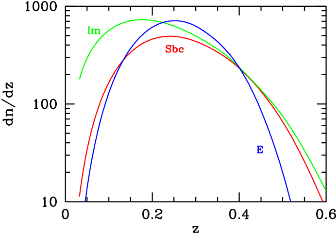
Figure 2.— Contributions to the full $dn/dz$ from different galaxy types in the apparent magnitude bin $19<r^{*}<20$ (other bins show similar trends). Each type is representative of one of the classes of galaxies for which CNOC2 derived Schechter fits (Im with Late; Sbc with Intermediate; and E with Early). Here the relative normalizations are important since the total $dn/dz$ (the blue curve in Figure 3) is the sum of these three individual contributions.

The total redshift distribution in a given magnitude bin is the sum of the contributions from all three galaxy classes. The resulting distributions are shown in Figure 3 for the four magnitude bins under consideration. We will refer to these as the direct CNOC2 $dn/dz$’s to distinguish them from the fits to Eq. [1]. As we will see shortly, Eq. [1] is not a perfect fit to the direct $dn/dz$. However, we will show below that this difference between the direct $dn/dz$ and the empirical fit has a negligible effect on the derived power spectrum.

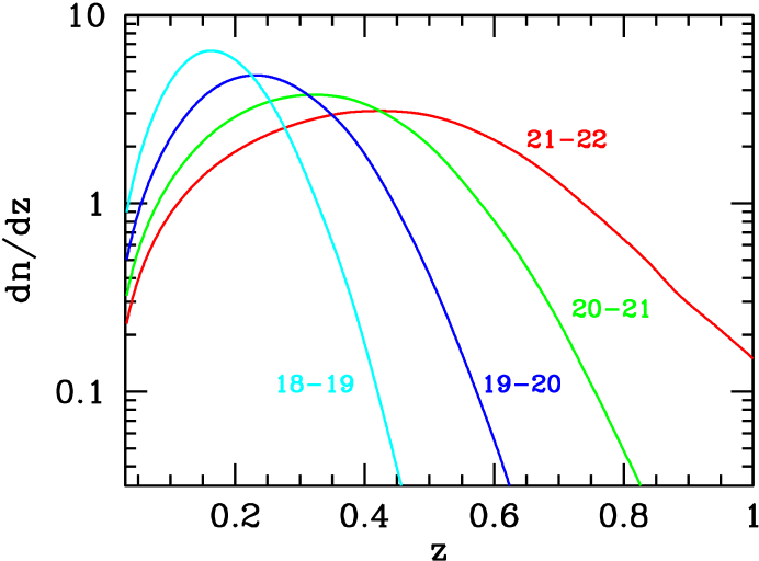
Figure 3.— Galaxy redshift distributions in four apparent magnitude bins using the CNOC2 selection function. All curves here (unlike those in Figure 2) are normalized so that $\int dzdn/dz=1$.

Figures 2 and 3 use the best-fit values of the Schechter function parameters from CNOC2. These parameters undoubtedly have correlated errors, although the correlation coefficients are not reported by CNOC2. Therefore, we neglect the correlations between the Schechter parameters, and derive a conservative estimate of the uncertainty in $dn/dz$ due to the uncertainties in the luminosity function, using one hundred Monte-Carlo runs. In any Monte-Carlo run, we choose each Schechter parameter from a Gaussian distribution with mean equal to the best fit value and standard deviation equal to the error reported by CNOC2. In a given run, we then compute the median redshift $z_{m}$ of the galaxy redshift distribution. The second column in Table 1 shows the median redshift $z_{m}$ (obtained from the best fit values of the Schechter parameters) and a standard deviation for each magnitude bin; the standard deviations are measured from the hundred Monte-Carlo runs. We emphasize that this is a very conservative estimate of the uncertainty in $dn/dz$, as it neglects the correlations in the errors of the Schechter parameters.

TABLE 1

Median redshift $z_{m}$ in the four magnitude bins computed using three different methods

Magnitude Bin	CNOC2	CFRS+SDSS	SDSS Photo-$z$
$18-19$	$0.17\pm 0.014$	0.17	0.20
$19-20$	$0.24\pm 0.025$	$0.25$	$0.26$
$20-21$	$0.33\pm 0.037$	$0.35$	$0.33$
$21-22$	$0.43\pm 0.062$	$0.46$

Figure 4 plots a set of $dn/dz$ from Eq. [1] in the magnitude bin $20<r^{*}<21$. The apparent discrepancy between the fit and the direct CNOC2 redshift has a negligible effect on the derived power spectrum. We will show this by using both $dn/dz$’s when computing the power spectrum; we will see that the differences in the derived power spectra are much smaller than the error bars (see Figure 11 in §4). Apparently, noticeably different radial galaxy distributions project the 3D clustering the same way on the sky as long as their median redshifts are the same.

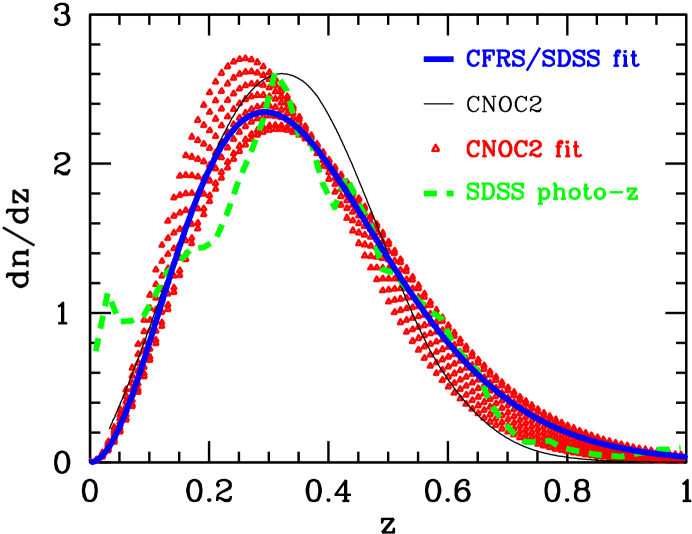
Figure 4.— Redshift distributions in the magnitude bin $20<r^{*}<21$. Thin black curve is the direct CNOC2 result; red triangles span the $1-\sigma$ range associated with the fit of Eq. [1] with $z_{m}=0.33\pm 0.037$; thick blue curve is best fit of Eq. [1] to CFRS+SDSS data; dashed green curve uses the photometric redshifts from SDSS.

2.2. CFRS+SDSS

The Canada-France Redshift Survey (CFRS, Lilly et al. 1995) is a deep redshift survey (with median redshift $z_{m}\approx 0.6$) of about $10^{3}$ faint galaxies, evenly subsampled in the magnitude range $17.5<I(AB)<22.5$. These galaxies were selected from five survey fields, each of area $10^{\prime}\times 10^{\prime}$, and also have deep $V$ and $I$ band isophotal photometry. The galaxy photometry was carried out using a limiting isophote of $\mu_{AB}(I)=28\$mag  arcsec^-2, and therefore would be expected to contain almost all of the light. We used an empirical relation $r_{\rm SDSS}=I_{\rm CFRS}+0.5*(V-I)_{\rm CFRS}$ derived using 130 galaxies that were imaged by both SDSS and CFRS, to estimate the $r^{*}$ band magnitude of all the CFRS galaxies that also have redshifts. We fit a third order polynomial for the median redshifts of the galaxy distribution as a function of $r^{*}$ $[z_{m}(r^{*})]$ in the magnitude range $17<r^{*}<22$, using the SDSS redshifts in the magnitude range $17<r^{*}<17.6$ and the CFRS redshifts at $19<r^{*}<22$. Finally, we determined the median redshift of galaxies in each unit magnitude bin in the magnitude range $18<r^{*}<22$ by multiplying this $z_{m}(r^{*})$ with a third order polynomial fit to the galaxy number counts as a function of magnitude in the SDSS (Yasuda et al. 2001) in the magnitude range $18<r^{*}<22$. The median redshifts in the four unit magnitude bins are given in Table 1; they agree remarkably well with the CNOC2 estimates. The agreement is impressive especially since each data set has its own limitations. While CFRS is a deeper survey over a smaller area, CNOC2 has no redshifts greater than $0.55$ (more precisely, their Schechter fits are valid only for $z<0.55$ since their efficiency falls steeply beyond this redshift). The fit in the magnitude bin $20-21$, shown in Figure 4, is consistent with the CNOC2 results.

2.3. Photometric Redshifts

Redshifts for the SDSS photometric data were estimated directly from the $u^{*},g^{*},r^{*},i^{*}$ and $z^{*}$ galaxy photometry. The technique used in this analysis is a hybrid between the empirical approach of fitting a polynomial relation between the colors and redshifts of galaxies (Connolly et al 1995) and techniques that model the colors of galaxies as a function of redshift using a priori galaxy spectral energy distributions (Fernandez-Soto et al 1999, Sawicki et al 1997). In our approach, we compare the colors of the galaxies with those predicted from galaxy spectral templates but we construct these templates from a sample of galaxies with high signal-to-noise photometry and spectroscopic redshifts (Connolly et al. in preparation). In this way, we can construct templates that are designed to match the observed colors of galaxies within a particular data set. The training techniques employed in this analysis are described by Csabai et al (2000) and Budavari et al (2000). The training of the spectral templates was based on $5,000$ SDSS galaxies (with measured redshifts) supplemented with $700$ galaxies with redshifts from the CNOC2 survey, for which we have SDSS photometry. For the trained spectral templates the dispersion within the photometric redshift relation is $\sigma_{z}\approx 0.07$ for $r^{*}<19$ and $\sigma_{z}\approx 0.12$ for $r^{*}<21$. All galaxies with photometric redshifts have associated errors and spectral types.

The redshift distribution from photo-$z$ is shown in the magnitude bin $20-21$ in Figure 4. In the regime of interest it agrees well with other estimates; the small fluctuations at $z<0.2$ probably arises from large scale structure in the galaxy distribution. Table 1 presents the median redshift in all magnitude bins except the faintest bin, where we are limited by the uncertainties in evolution of the galaxy population.

3. Kernels

The angular correlation functions in real and Fourier space are related to the 3D power spectrum (e.g. Peebles 1980; Eisenstein & Zaldarriaga 2000) by

$$\left(\matrix{w(\theta)\cr l^{2}C_{l}}\right)=\int_{0}^{\infty}dk\,k\,P(k,z=z_{m})\left(\matrix{K_{w}(k\theta)\cr K_{C_{l}}(k/l)}\right)$$ (6)

in the small angle approximation. Here, $z_{m}$ is the median redshift of the galaxy distribution in a given magnitude bin in the angular photometric catalog. The kernel for $w$ is

$$K_{w}(k\theta)={1\over 2\pi}\int_{0}^{\infty}dz(d\chi/dz)J_{0}(k\theta\chi(z))\left[(dn/dz)(dz/d\chi)\right]^{2}E(z,z_{m}).$$ (7)

Here, $\chi$ is the comoving distance out to redshift $z$; $J_{0}$ is the Bessel function of order zero; $dn/dz$ is the redshift distribution of galaxies, normalized so that the integral of $dn/dz$ over all $z$ is one; and $E(z,z_{m})$ is a function which describes the redshift evolution of density fluctuations between the redshifts $z_{m}$ and $z$. In principle $E$ is quite complicated, with a scale ($k$) dependence as well. However, for all practical purposes the current data are not sensitive to this evolution (Scranton & Dodelson 2000), so we set $E=1$. In other words, the angular clustering in a given magnitude bin is determined by the 3D clustering at the median redshift associated with that bin. Thus, when we invert the angular correlations to obtain the 3D power spectrum, we should keep in mind that the different spectra obtained from the different magnitude bins correspond to different redshifts. We assume a flat, $\Lambda$ dominated Universe with $\Omega_{\Lambda}=0.7$. The kernel $K_{w}(k\theta)$ is shown in Figure 5 for the four magnitude bins. The largest contribution to $w(\theta)$ comes from scales on the order of the first zero, e.g. for $21<r^{*}<22$, at $k\sim 0.002{\rm h\ Mpc}^{-1}/\theta$, and a factor of three smaller scale at $k\sim 0.006{\rm h\ Mpc}^{-1}/\theta$ in the $18<r^{*}<19$ bin. Thus, as anticipated, the angular correlations of galaxies at a given angle in the faint magnitude bins probe larger scales (smaller $k$) than do those in the bright magnitude bins.

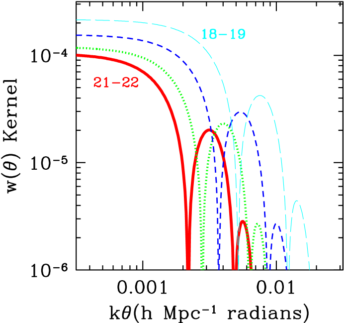
Figure 5.— Absolute value of the kernel for the angular correlation function $w(\theta)$ in four different magnitude bins. At left, faintest bin ($21<r^{*}<22$) is lowest, up to the brightest bin ($18<r^{*}<19$) on top. The sign of the kernel starts positive at small $k$ and changes with each oscillation.

The kernel for $C_{l}$ is simpler (again, in the small-angle approximation)

$$K_{C_{l}}(k/l)=\left[\chi E(z,z_{m})\Big{(}{dn/dz)(dz/d\chi)}\Big{)}^{2}\right]_{\chi=l/k}.$$ (8)

Both of these kernels $K_{w}$ and $K_{C_{l}}$ should be generalized to large angles, once the angular correlations are measured on large angular scales. However, the current measurements of angular clustering in the galaxy distribution are on small enough scales that these small angle expressions remain valid (see e.g. T01). Figure 6 shows the kernels $K_{C_{l}}$ in the four magnitude bins. Here, it is easier to see (as compared with the $w$ kernels) that (a) the kernel $K_{C_{l}}$ has a single peak showing that the $C_{l}$ on a given angular scale gets most of its contribution from the 3-dimensional correlations on a given physical scale, and (b) this physical scale is larger for fainter magnitude bins (since the peak moves to the left) than for brighter bins. Another feature which makes the $C_{l}$’s easier to interpret is that the kernel is always positive.

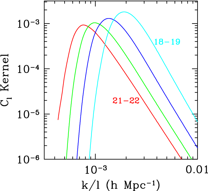
Figure 6.— Kernel for the 2D power spectrum ($K_{C_{l}})$ in four magnitude bins. The kernel for galaxies in the faintest magnitude bin is the one to the farthest left, since faint galaxies probe larger physical scales at a fixed angular scale.

The uncertainty in $dn/dz$ leads to a corresponding uncertainty in the kernels. It is most instructive to consider this resulting uncertainty in the $C_{l}$ kernel since it is a relatively simple function. Figure 7 shows the level of this uncertainty in $K_{C_{l}}$. Using the parameterization of Eq. [1], we can change the distribution by varying the parameter $z_{m}$. When $z_{m}$ is small, a given angular scale subtends a small physical scale. Hence the kernel peaks at large $k/l$ (for fixed $l$, the wavenumber $k$ is large). As $z_{m}$ increases, a given angular scale subtends a larger physical scale. We therefore see the kernel shift to the left in Figure 7. Besides this lateral shift, the amplitude decreases as $z_{m}$ increases. To get the same angular clustering strength, one needs a larger 3D power spectrum as the median redshift of the galaxies increases to avoid cancellations of over- and under-densities along the line of sight. Also shown in Figure 7 is the shift in $K_{C_{l}}$ arising from a different background cosmology. The peak of the kernel in a flat, matter-dominated Universe shifts towards smaller scales. This is to be expected, as a flat $\Lambda-$dominated Universe has “more volume” at a given redshift. Therefore, the physical distance separating galaxies at a given $z_{m}$ is larger in a $\Lambda-$Universe. Clustering on a given angular scale therefore probes larger physical scales (smaller $k$) in a $\Lambda-$Universe. The amplitude of the kernel decreases as $\Lambda$ is introduced because there are more cancellations in the density inhomogeneities along the line of sight.

Figure 7.— The sensitivity of the angular kernel (in the magnitude bin $20<r^{*}<21$) to uncertainties in the redshift distribution and cosmology. Heavy solid (red) curve corresponds to the best fit of Eq. [1], with $z_{m}=0.33$. Thin (red) curve shows the effect of increasing $z_{m}$ by $1-\sigma$. Dashed (blue) curve shows the effect of modifying the underlying cosmology, and corresponds to the kernel in a flat, matter-dominated Universe. It has the same $z_{m}$ as the heavy red curve.

4. The 3D Power Spectrum

The Automated Plate Machine (APM; Maddox et al. 1990) survey a decade ago ushered in a renewed interest in techniques for inverting the angular correlation function to extract the 3D power spectrum. Efstathiou and Baugh (1993) used Lucy’s Method to accomplish this inversion; Dodelson and Gaztanaga (2000) used a Bayesian prior constraining the smoothness of the power spectrum to stabilize the inversion; most recently, Eisenstein and Zaldarriaga (2000, hereafter EZ) used a Singular Value Decomposition to eliminate modes that destabilize the inversion.

The good news is that all these techniques “work.” They have been tested using numerical simulations and against each other and generally they get similar results for the power spectrum. The more subtle issue has been a correct estimate of the errors on the derived power spectrum. Perhaps most important, as mentioned by Dodelson and Gaztanaga (2000) and then illustrated persuasively by EZ, errors on $w(\theta)$ measurements in different angular bins are highly correlated. EZ showed that accounting for these correlations is crucial if one wants to report reliable errors bars on the 3D power spectrum. This flurry of activity, along with parallel activity in map-making (another form of inversion in the field of Cosmic Microwave Background anisotropies; see e.g. Bond et al. 1999 for an overview) has taken the inversion process to a higher level of sophistication and reliability.

The starting point for inversion is the relation between the measured angular clustering of galaxies and the 3D power spectrum, the main component of which is the kernel. The integral in Eq. [6] can be written in matrix form as

$$d={\bf K}P+n$$ (9)

where $d$ is an $N_{d}$ dimensional vector containing the data, either the angular correlation function $w(\theta)$ (in which case each component of the vector corresponds to $w$ in a given angular bin) or the 2D power spectrum $C_{l}$ (with each component the power in an $l-$bin). The kernel ${\bf K}$ is an $N_{d}\times N_{P}$ matrix, $N_{P}$ being the number of bins in 3D wave number $k$ in which we are attempting to estimate the power spectrum $P$. Note that ${\bf K}$ is related to, but not identical to the kernels of Eq. [6], due to the extra factor of $k\,dk$. In addition to the signal (the first term in Eq. [9]), the data points (measurements) also contain some noise, characterized by the noise vector $n$. We take this noise to be drawn from a distribution with mean zero and variance given by the covariance matrix, $C_{d}$. The covariance matrix for $w$ is discussed in detail in Sc01, that for $C_{l}$ in T01.

Following EZ, we re-define the data and power spectrum vectors. The data is renormalized by the noise:

$$d^{\prime}\equiv C_{d}^{-1/2}d$$ (10)

where $C_{d}^{-1/2}$ is the matrix with the property $C_{d}^{-1/2}C_{d}^{-1/2}=C_{d}^{-1}$. Roughly, $d^{\prime}$ is the signal to noise ratio of the actual data points (this is easiest to see in the unrealistic case that the correlation matrix of the noise is diagonal). The power spectrum is also renormalized, weighted by some fiducial spectrum $P_{\rm norm}$:

$$P^{\prime}\equiv{P\over P_{\rm norm}}.$$ (11)

With this renormalization, all the elements of the vector $P^{\prime}$ will be of order unity; large deviations can be flagged. We set the fiducial spectrum to be that of a $\Lambda CDM$ model, with parameters identical to those used in the simulations described in Sc01 (e.g. $\Omega_{\Lambda}=0.7$). although our final results are insensitive to this choice. In terms of these renormalized variables, the relation between data and signal (Eq. [9]) becomes

$$d^{\prime}={\bf K}^{\prime}P^{\prime}+n^{\prime}$$ (12)

with the renormalized kernel equal to

$${\bf K}^{\prime}=C_{d}^{-1/2}{\bf K}P_{\rm norm}.$$ (13)

The renormalized noise $n^{\prime}=C_{d}^{-1/2}n$ has covariance matrix equal to the identity matrix (since $<nn>=C_{d}$). The new kernel ${\bf K}^{\prime}$ is roughly the expected signal (${\bf K}P_{\rm norm}$) divided by the noise. Therefore, modes with eigenvalues of ${\bf K}^{\prime}$ greater than one have large signal, while modes with very low weight are not expected to yield much information on the power spectrum.

With these redefinitions, the minimum variance estimator of the power spectrum is

$$\hat{P^{\prime}}=C_{P^{\prime}}{\bf K}^{{}^{\prime}t}d^{\prime}$$ (14)

with the associated error matrix

$$C_{P^{\prime}}=\left({\bf K}^{{}^{\prime}t}{\bf K}^{\prime}\right)^{-1},$$ (15)

where ^t means transpose. To get back to $P$ and its covariance matrix, one simply multiplies each element of $\hat{P^{\prime}}$ by the corresponding element of $P_{\rm norm}$ and each element of the matrix $C_{P^{\prime},ij}$ by $P_{{\rm norm},i}P_{{\rm norm},j}$. If we include all the modes associated with the rows of ${\bf K}^{\prime}$, then $P_{\rm norm}$ has absolutely no effect on the inversion. Only when we begin eliminating modes with low signal-to-noise ratio (as described below) does the choice of $P_{\rm norm}$ have any impact.

In practice, the estimator of Eq. [14] is not always stable: very small changes in the input data lead to huge variations some elements of $P^{\prime}$. EZ (and other groups making maps from Cosmic Microwave Background timestreams) showed that an easy way to handle this instability is to use Singular Value Decomposition, wherein the matrix ${\bf K}^{\prime}$ is decomposed as

$${\bf K}^{\prime}=UWV^{t}$$ (16)

where $U$ is a column orthonormal matrix, $W$ is a diagonal matrix, and $V$ is orthogonal. The weights, the diagonal elements of $W$, then are measures of signal-to-noise ratio. Very small weights are responsible for the instability of the inversion.

One form of instability is particularly easy to treat. If the eigenmode with a very low weight can be identified with a single $k$ bin, then we eliminate the low weight by simply removing the $k$ bin. We then redo the inversion without the offending bin. Especially in the case of $w(\theta)$ inversion we will see that this way of tweaking the choice of $k$ bins eliminates much of the instability. An example of this process is illustrated in §4.1.

As we will see below, this improved choice of $k$ bins does not work as well on the $C_{l}$ data of T01. In that case, the low weight modes are typically linear combinations of many different modes, so it is impossible to identify one offending $k$ bin. EZ give a recipe for eliminating the deleterious effects of these low weights, which involves rescaling them higher when computing the covariance matrix $C_{P^{\prime}}$. We follow this recipe here, eliminating modes with weight less than unity (note that this is where our choice of fiducial power spectrum enters into the analysis). Since the weight is a measure of signal to noise, we are effectively eliminating from the analysis the noisiest modes. This should not have any impact on the final parameter determination.

4.1. Inversion of $w(\theta)$

We use the measurements of $w(\theta)$ and its covariance matrix as presented in Sc01 and C01. We use the measurements on angles larger than $0.01$ degrees, leaving us with $19$ angular bins.

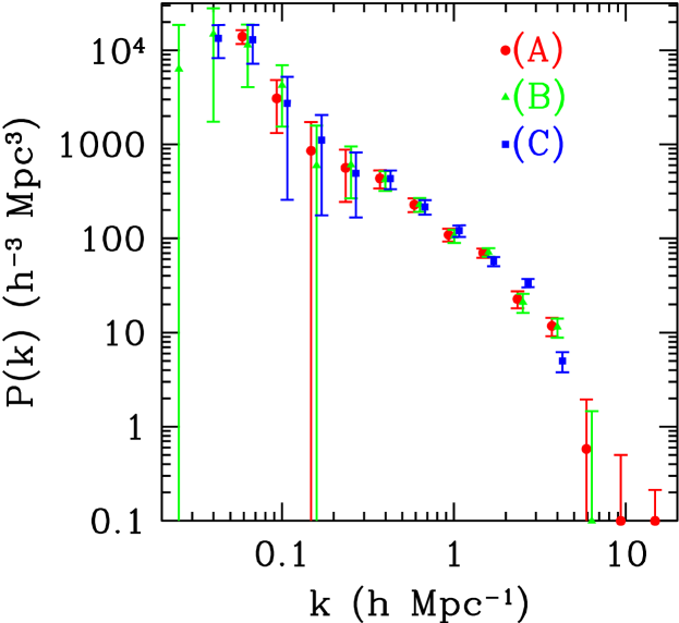
Figure 8.— The power spectrum inferred from the bin $21<r^{*}<22$. The three different results correspond to three different choices of $k$ bins. First attempt (A) is the set depicted with red circles; second (B), adding two low $k$ modes and dropping two high $k$ modes, with green triangles; final (C), dropping a $k$ mode on each end, with blue squares.

Let us illustrate the Singular Value Decomposition with the $21<r^{*}<22$ magnitude bin. For this bin, the kernel in Figure 5 starts to fall off when $k\theta\sim 2\times 10^{-3}$h Mpc^-1 radians. For a fixed angle $\theta$, the integral over $k$ in Eq. [6] is dominated by the value of the kernel in this region. Therefore, the smallest angular bin considered here, $\theta=0.01^{\circ}$, is sensitive to the power spectrum around the wavenumber $k\sim 2\times 10^{-3}$h Mpc${}^{-1}/1.7\times 10^{-4}\sim 10$h Mpc^-1. Similarly, the largest angular scale with a significant measurement of $w(\theta)$, around one degree, probes the power spectrum at wavenumbers of order $k\sim 0.1$h Mpc^-1. Our first choice of $k$ bins with which to fit the power spectrum, therefore, spans the range $k=0.1-10$h Mpc^-1. As shown in Figure 8, we actually try bins with a slightly broader range. The initial choice, labeled (A) in Figure 8, goes as low as $0.06$h Mpc^-1 and as high as $15$h Mpc^-1. The results shown with this set of bins are after the rescaling of the two low weights. We wish to avoid such rescaling though, so let us try to understand the origin of the low weights.

Figure 9 shows the eigenvectors corresponding to thirteen different weights of binning scheme (A), and their sensitivity to wavenumber. The two modes with largest weights (at the top) measure linear combinations of the power in the range $k\sim 0.1\rightarrow 1\$h Mpc^-1. The next six modes also probe this region, but these modes also extend to smaller and larger scales. Note, though, that the ten modes with the highest weights have little sensitivity to the power spectrum in the last two bins, at $k=8{\rm\ and}\ 15h$ Mpc^-1. They are however sensitive to the largest scales in this binning scheme. We can also see this from the small error bars on the left-most red point in Figure 8. It is therefore natural to add a couple of bins at smaller $k$ and see whether any information can be obtained on very large scales.

Figure 9.— Eigenmodes of the renormalized kernel in the magnitude bin $21<r^{*}<22$. Left column shows all thirteen modes corresponding to $k$ binning scheme (A) in Figure 8; right column shows all eleven modes corresponding to scheme (C). Modes are plotted two at a time for clarity, with the dashed line corresponding to the mode with lower weight. The numbers inside the panels are the weights of the two modes.

The second scheme (B) in Figure 8 therefore adds two bins at $k=0.03,0.05$ h Mpc^-1 and drops the two highest $k$ bins, which we have identified with low weight modes. The measurement is indeed sensitive to the power in these two large scale bins. It is also encouraging that the additional bins do not affect the determination of the power anywhere else by more than about half a standard deviation. It is clear then that our initial rough guess of the range to which $w(\theta)$ is sensitive was slightly incorrect: there is little sensitivity at the highest $k$ we chose, but we underestimated the large scale information. We still want to avoid rescaling weights, so we drop two more bins for our third and final binning scheme. The right panels in Figure 9 show the eigenvectors corresponding to these eleven modes and their $k$ dependence. The highest weight modes are identical to those on the left (signs are irrelevant here). All modes have weights greater than unity; therefore the inversion is stable.

It is important to make explicit the most important feature of Figure 8, namely, the estimate of the power spectrum is robust to reasonable changes in our choice of the $k$ bins.

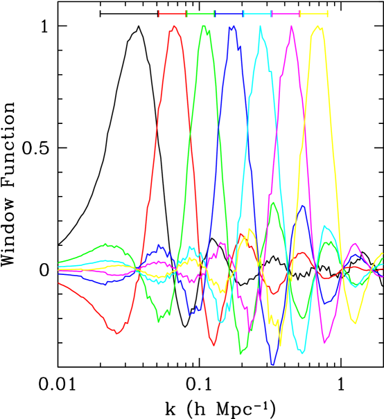
Figure 10.— Window functions for the first seven $k$ modes in $21<r^{*}<22$. The flat bands on top of each window function correspond to the range of $k$ used in estimating the power in each mode. All the window functions have been normalized to unity.

Until now, we have been thinking of the power spectrum measured using Eq. [14] as the best fit estimate of the power in a given band, assuming that the true power spectrum was flat in that band. While this is correct, it is also not very useful, since realistic power spectra are not flat within the finite width of the $k-$ bands of interest. Another way of understanding these spectra therefore is to note that the estimator in Eq. [14] is yet another in a series of quadratic estimators (quadratic in the galaxy overdensities; see e.g. Tegmark et al. 1998 and the discussion in Appendix A of T01). Any quadratic estimator has associated with it a window function that relates it to the true power spectrum, and the one in Eq. [14] is no exception. In this case, the window function is

$${\cal W}=C_{P^{\prime}}K^{{}^{\prime}t}K^{\prime}_{\infty}$$ (17)

where $K^{\prime}_{\infty}$ is $K^{\prime}$ extended to infinitely many $k$ bins that are infinitesimally narrow. In the limit that $K^{\prime}$ is equal to $K^{\prime}_{\infty}$, the window function is simply equal to the identity matrix. The finite binning changes this. Some window functions for the faintest magnitude bin are shown in Figure 10. Note that they quite accurately probe the window for which they were constructed. The oscillating lobes of each window function remove power outside the band of interest. These window functions must be used when comparing model power spectra to the band power estimates presented here.

Let us now return to the question of ambiguity in the kernel arising from the uncertainties in the galaxy redshift distributions. The fit of Eq. [1] to the direct CNOC2 $dn/dz$ appears only marginal in Figure 4. Figure 11 compares the power spectrum derived using the direct CNOC2 $dn/dz$ and the fit in equation Eq. [1], in the faintest magnitude bin $21<r^{*}<22$. The power spectra using these two $dn/dz$’s agree very well over the entire range of wavenumbers, showing that our estimates of the power spectrum are not very sensitive to the exact details of $dn/dz$.

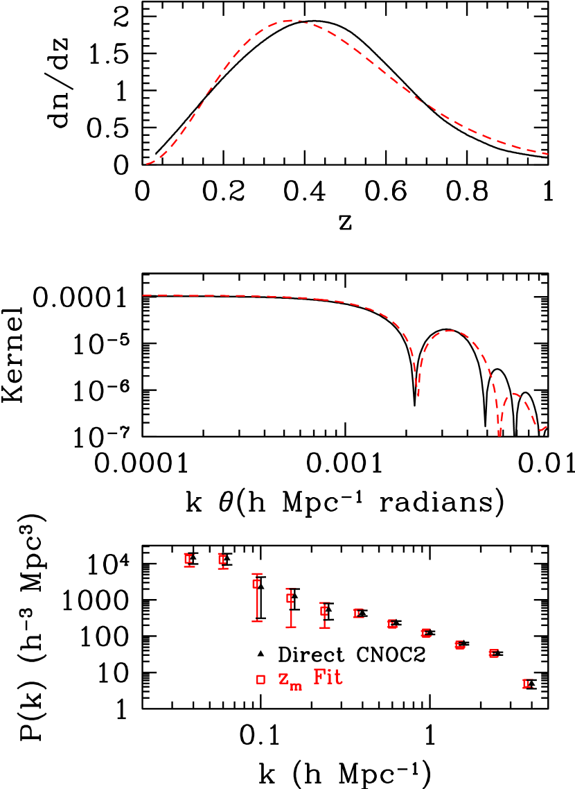
Figure 11.— The result of fitting $dn/dz$ to the simple form of Eq. [1]. Black solid curves are the direct CNOC2 result, red dashed from Eq. [1] with $z_{m}=0.43$ (all panels show $21<r^{*}<22$). Top panel: Noticeable difference in $dn/dz$. Middle panel: How this small difference affects the kernel. Bottom panel: The final impact on the power spectrum is negligible.

The fit to Eq. [1] therefore is adequate for our purposes. We can use it to quantify the uncertainty in the galaxy redshift distribution. In each magnitude bin, we account for the errors in $z_{m}$ and propagate these forward to estimate the errors on the power spectrum. To do this, we generate one hundred different $z_{m}$’s from a Gaussian distribution with mean and standard deviation given in Table 1 (e.g. in the magnitude bin $21-22$, the mean is $0.43$ and standard deviation $0.062$). For each of these redshift distributions, we generate a kernel and compute the power spectrum from the $w(\theta)$ data. The spread in these hundred estimates of the power spectra define a covariance matrix. This new covariance matrix is then added to the one defined in Eq. [15].

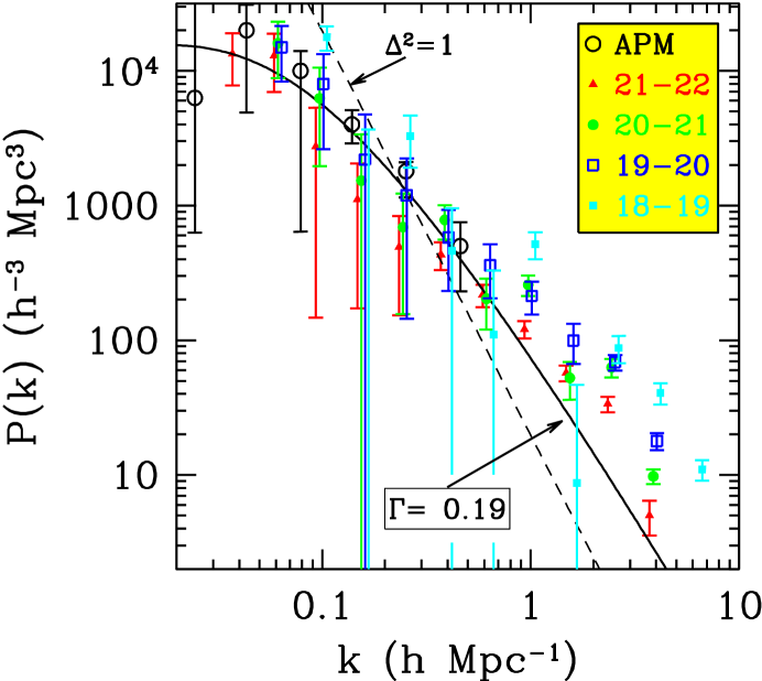
Figure 12.— The 3D power spectrum from angular data in four magnitude bins. Also shown is the maximum likelihood power spectrum from the APM survey (Efstathiou & Moody 2000). The dashed line, defined by $\Delta^{2}\equiv 4\pi k^{3}P/(2\pi)^{3}=1$, delineates the linear from the non-linear regime, while the solid line is the best fit linear spectrum from Sz01. The parameter $\Gamma$, introduced by Bardeen et al. (1986) determines the shape of the power spectrum.

Figure 12 shows the power spectrum from each of the four magnitude bins. Also shown in Figure 12 are the results from the inversion of the APM angular data by Efstathiou and Moody (2000). The two estimates of the power spectrum agree very well in the overlapping wavenumbers $0.03<k/{\rm h\ Mpc}^{-1}<0.3$. Figure 12 suggests that the power spectrum in the fainter bins is smaller than in the brighter bins. This is especially apparent for large $k$, in the non-linear regime. This realization is consistent with the fits of T01, which require larger bias factors in the brighter bins.

There are several possible causes of this difference in power. The first relies on the observation that the estimate from each magnitude bin samples the power at a different redshift. The median redshift for galaxies in the faintest bin is of order $z\simeq 0.43$, while the galaxies in the brightest magnitude bin reside at redshift $z<0.2$. Power in hierarchical models cascades down from large to small scales as non-linearities become prominent. Therefore, we expect less power at earlier times especially on non-linear scales. Thus, consider the power spectrum in the $k=.252$h Mpc^-1 bin. The linear regime is usually associated with scales larger than those on which $\Delta^{2}\equiv 4\pi k^{3}P/(2\pi)^{3}=1$. The two faintest magnitude points at $k=.252$h Mpc^-1 both have $\Delta^{2}$ significantly smaller than unity, while the APM point and that from our brightest magnitude are non-linear. Indeed, the usual cut-off between linear and non-linear scales lies in the wavenumber range $0.1<k/{\rm h\ Mpc}^{-1}<0.2$, so the linearity observed in our faintest magnitudes suggests we are indeed observing the Universe at earlier times when galaxies were less clustered.

Another possible cause of the difference in the power spectrum in different magnitude bins is the bias between galaxies and mass. More luminous galaxies tend to be in clusters and therefore have a stronger power spectrum. This may be part of the explanation for the larger power in the brighter magnitude bins.

Table 2 gives numerical values of the power spectrum in each of the four magnitude bins, with two sets of errors. The first is the total error including the uncertainty in $dn/dz$, the second (in parentheses) neglects this uncertainty.

TABLE 2

3D Power spectrum in 4 magnitude bins.

k (h Mpc-1)	P(k) (h-3 Mpc3) $\pm dP$ ($dP$ no $dn/dz$ uncertainty)
	18-19	19-20	20-21	21-22
$0.040$				$13409\pm 5614(5130)$
$0.063$		$14908\pm 6604(4887)$	$16016\pm 7168(3507)$	$12916\pm 5962(5711)$
$0.100$	$17746\pm 3609(3138)$	$7956\pm 5344(5201)$	$6246\pm 4292(3142)$	$2728\pm 2591(2480)$
$0.159$	$-3692\pm 3664(2929)$	$2191\pm 2569(2483)$	$1531\pm 1847(1511)$	$1112\pm 939(936)$
$0.252$	$3274\pm 1371(1187)$	$1191\pm 1047(967)$	$691\pm 535(519)$	$493\pm 340(326)$
$0.40$	$461\pm 492(464)$	$580\pm 348(338)$	$782\pm 222(191)$	$432\pm 101(98)$
$0.63$	$110\pm 218(182)$	$360\pm 155(127)$	$203\pm 83(69)$	$217\pm 41(38)$
$1.00$	$517\pm 117(75)$	$213\pm 58(56)$	$258\pm 45(30)$	$121\pm 17.8(16.7)$
$1.59$	$8.7\pm 38(29)$	$99\pm 32.8(20.9)$	$52.5\pm 16.3(15.5)$	$57\pm 7.6(6.4)$
$2.52$	$87.7\pm 19.9(10.6)$	$68.6\pm 9.0(6.9)$	$62.9\pm 10.0(5.8)$	$33.7\pm 4.4(3.4)$
$4.0$	$40.6\pm 7.3(4.1)$	$17.9\pm 2.6(1.6)$	$9.8\pm 1.2(1.1)$	$5.0\pm 1.4(1.2)$
$6.3$	$11.0\pm 1.9(1.2)$

The errors on the 3D power spectrum estimates in different $k$ bins are correlated. The error bars shown in Figure 12 are the marginalized errors, allowing the power in all other $k$ bins to vary freely. These are the square roots of the diagonal elements of $C_{P}$. The unmarginalized errors (inverse square root of the diagonal elements of $C_{P}^{-1}$) are often much smaller due to the correlations. Figure 13 illustrates the correlation matrix:

$$r_{ij}\equiv{C_{P,ij}\over\sqrt{C_{P,ii}C_{P,jj}}}$$ (18)

for the power spectrum extracted from galaxies in the four bins. Typically, adjacent $k$ bins are significantly anti-correlated. The correlation matrices in Figure 13 do not include the contribution from the uncertainty in $dn/dz$. Figure 14 shows the correlation matrices including this uncertainty. Note that, especially in the brighter bins, our estimate for the power on small scales is now coupled to the large scale estimate because of the uncertainty in $dn/dz$.

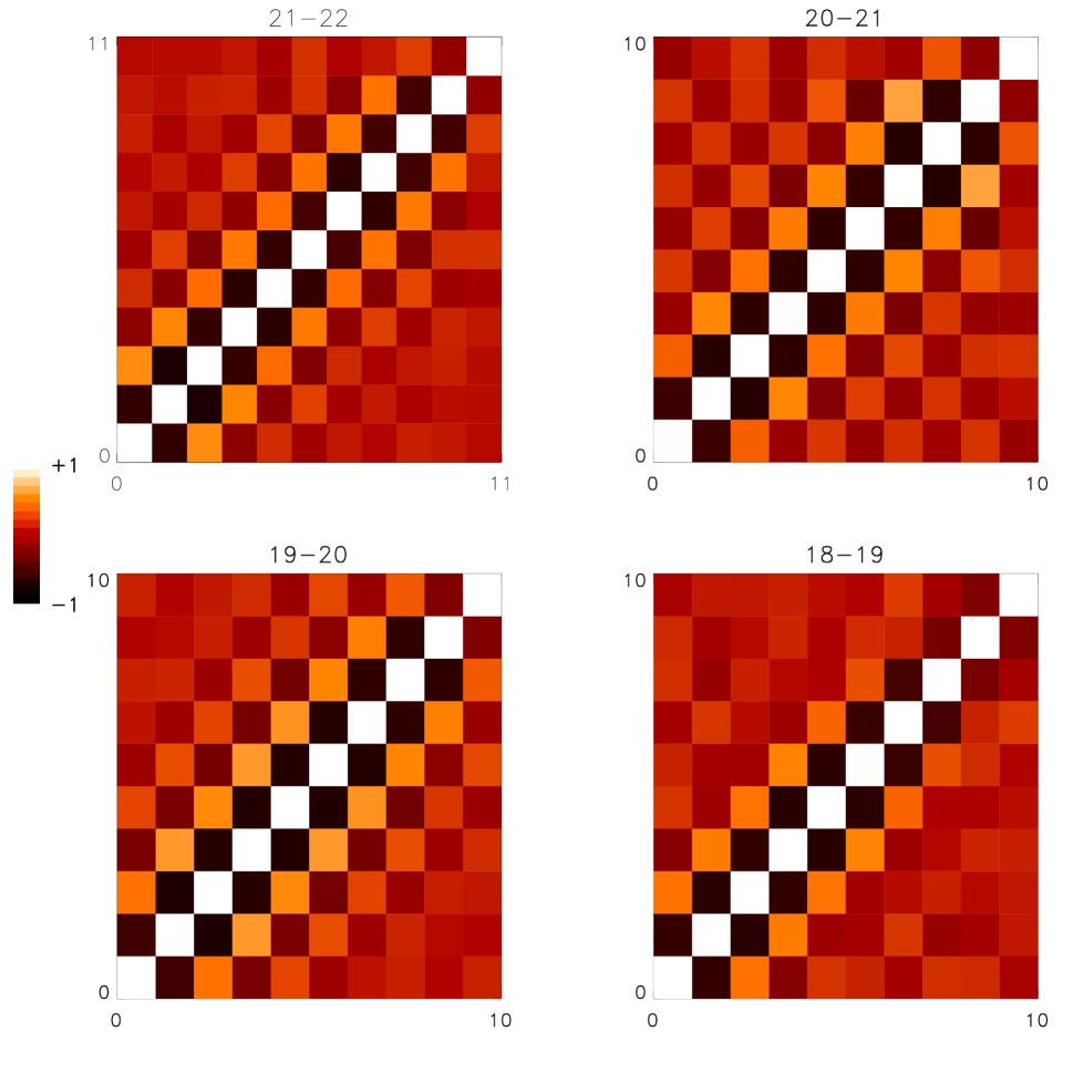
Figure 13.— Correlation matrix for the 3D power spectrum inferred from $w(\theta)$ in the four magnitude bins, neglecting the contribution from the uncertainty in $dn/dz$. Diagonal elements (all equal to one) run from bottom left to upper right. Elements in lower left are small $k$ (large scale) modes; e.g. bin labelled $0$ in upper left corresponds to $k=0.04$h Mpc^-1 as can be seen from Table 2. Adjacent $P(k)$ bins are anti-correlated at levels approaching $-1$.

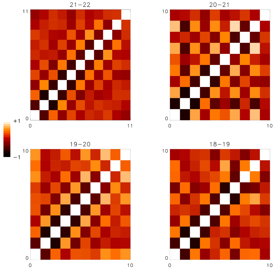
Figure 14.— Same as Figure 13 except that the correlation matrix includes the contribution from the uncertainty in $dn/dz$. This leads to enhanced correlations between small and large scales.

4.2. Inversion from $C_{l}$’s

We now estimate the 3D power spectrum from the angular power spectrum, the $C_{l}$’s, as presented in T01. The advantage of the inversion process in this case is more subtle than in the case of $w(\theta)$. To understand why, recall that inverting is equivalent to introducing the quadratic estimator of Eq. [14]. As we have seen, this estimator (Eq. [14]) has a window function associated with it. Looking back to Eq. [9], though, we see that $C_{l}$ (or $w(\theta)$) itself is also a quadratic estimator of the power spectrum, with the window function equal to the kernel, $K^{\prime}$. Let’s call this window function the observational window function to distinguish it from that of Eq. [17]. The observational window function for $w(\theta)$ is not positive definite and is not sharply peaked around a particular wavenumber (recall Figure 5). The observational window function for $C_{l}$ on the other hand does suggest that each $l-$ band can be associated with a given range in $k$. So $C_{l}$ itself is a useful estimator of the power spectrum. Why invert then? Inversion is still important, even for the $C_{l}$’s, because the window functions associated with the estimator of Eq. [14] are more sharply peaked than the observational window functions.

Figure 15 illustrates this point. For three different $k$ modes, the window functions associated with Eq. [14] are plotted along with the observational window functions. The estimator of Eq. [14] tries to remove all power outside the bin of interest by introducing modulations of the power. The power estimated through the inversion process therefore gets very little leakage from higher or lower wavelength modes. This contrasts with the observational window functions, which are relatively broad and do pick up power from a wide range of scales. This feature is particularly important if one is interested in using the power spectrum estimates for parameter determination. In that case, one typically wants to restrict the analysis to the largest scales, which are least affected by non-linearities and scale dependent galaxy bias. The narrow window functions arising from inversion facilitate this restriction.

We fit the fourteen measurements of $C_{l}$ with fourteen $k$ bands. This binning allows for easy comparison with the observational window functions, but it leads to more instability in the inversion (many modes are undetermined). This shows up in Figure 15, where the lowest $k$ window has been shifted over significantly to smaller scales (larger $k$) as compared with the corresponding observational window. This shift is due to the elimination of low weight modes in the SVD. Since the largest scale modes have very little weight, the effective window moves to smaller scales that are better probed by the angular data.

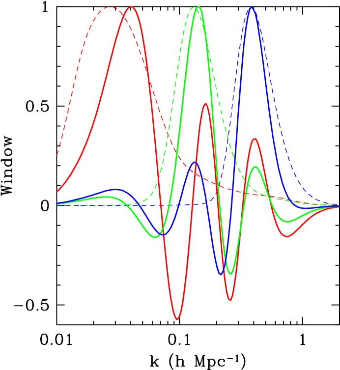
Figure 15.— Window functions for 3D power spectrum from the $C_{l}$’s. Solid curves are the windows defined via Eq. [14]; dashed are the windows for the $C_{l}$’s themselves (equivalent to those in Figure 6 of T01). Three different $k$ modes are shown here.

The estimates of the power spectrum from the $C_{l}$’s are shown in Figure 16. They do not extend to scales as small as those probed by $w(\theta)$ because it is computationally difficult to evaluate $C_{l}$ on small scales. The error bars appear large, but are deceptive for two reasons. First, adjacent bins are once again correlated, as indicated in Figure 17. The correlations are smaller than those we encountered when inverting $w(\theta)$ because, as emphasized by EZ, the $C_{l}$’s are uncorrelated in the all-sky limit, while the covariance matrix for $w(\theta)$ is intrinsically complicated. These covariances persist as we propagate errors through to the power spectrum. The second, and more important reason, for the large error bars in Figure 16 is that about twice as many bins were chosen in this case as compared with the $w(\theta)$ inversion, again to facilitate comparison with the observational window functions. We will see in §5 that the power spectrum from the $C_{l}$ inversion is almost as constraining as that from $w(\theta)$.

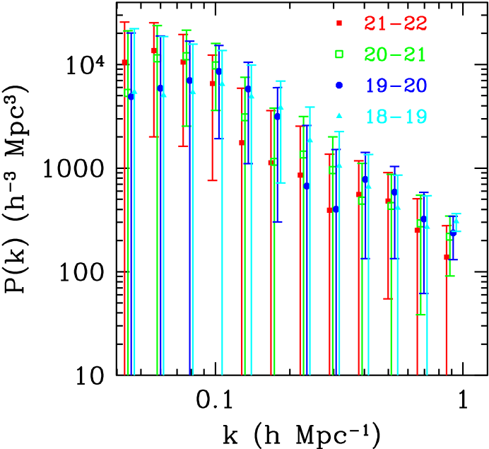
Figure 16.— Inferred power spectrum from the $C_{l}$’s.

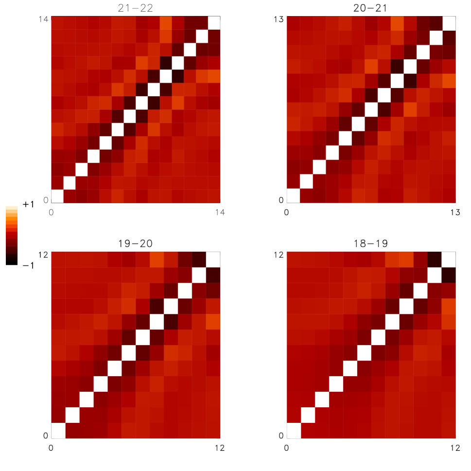
Figure 17.— Correlation matrices for $P(k)$ estimated from the $C_{l}$’s. Again bottom left corresponds to small $k$; top right to large $k$. These do not include the $dn/dz$ uncertainty.

The agreement with the power inferred from $w(\theta)$ is good, as shown in Figure 18. (Here we have used fewer $k$ bins to allow for easy comparison.) The unmarginalized errors are shown (primarily to keep the plots from getting too cluttered). The brightest bin shows how much larger the marginalized errors are in each case.

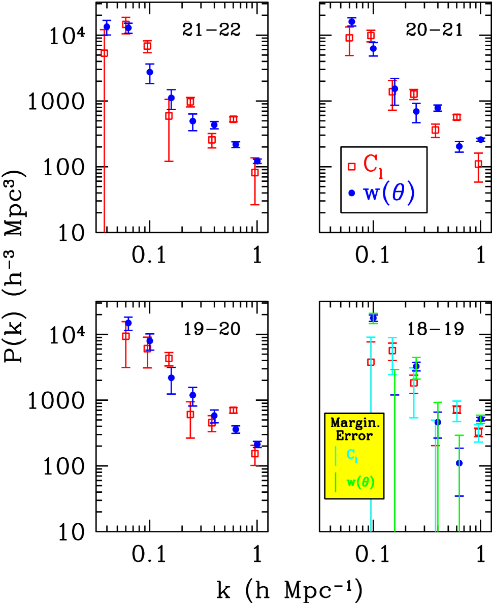
Figure 18.— Comparison of the power spectrum from $w(\theta)$ and from $C_{l}$ in the four magnitude bins. In this plot (and this plot only) error bars are unmarginalized errors; non-zero covariance between adjacent $k$ bins make marginalized errors much larger. Bottom right panel for brightest bin shows both errors.

The two measures of angular power, $w(\theta)$ and $C_{l}$, therefore, agree with each other. This is extremely reassuring given the long path in each case from raw data to angular power. The small differences are a result of the many different choices along each route. For example, the quadratic estimator used by Sc01 and C01 to measure $w(\theta)$ differs from that used by T01 to measure $C_{l}$. The latter assumes a prior power spectrum; in principle it handles edge effects more accurately. Nonetheless, the respective covariance matrices account for the efficiency of the estimator. T01 used a Karhunen-Loeve (KL) decomposition to measure $C_{l}$, in the process eliminating many low weight modes. In a similar vein, the pixelization in T01 was coarser than that of Sc01 and C01. Both these differences mean that $w(\theta)$ includes more small scale information since the low weight KL modes are small scale modes. We do not expect this to lead to any significant differences on large scales.

Perhaps the most difficult part of the computation in each case is the covariance matrix. The final (small) differences between the two sets of measurements are most likely due to the different ways of computing these error matrices. The $w(\theta)$ covariance matrix comes from the simulations of Scoccimarro & Sheth (2001). There are two worries with this approach: (i) the underlying model used in the simulations may not be correct and (ii) estimating the $N_{d}(N_{d}+1)/2$ elements from a finite number of simulations (in this case two hundred) is dangerous. The second worry is of particular concern because the off-diagonal elements are non-negligible. Sc01 however show that at least the diagonal elements of the covariance matrix agree with the Gaussian approximation on large scales. The $C_{l}$ covariance matrix was obtained assuming the perturbations are Gaussian. The worry here is that non-Gaussianities might be creeping in and, for example, inducing non-zero correlations among the different bands. T01 show, however, that the kurtosis is consistent with the Gaussian prediction, suggesting that contamination is unlikely. While these checks are reassuring, we believe that the small differences that remain are due to the uncertainties in the covariance matrix. Fortunately, these uncertainties will be less significant, at least on large scales, for the full SDSS data set which will go even deeper into the linear, Gaussian regime.

5. Conclusion

We have analyzed early photometric data from the SDSS and estimated the 3D power spectrum. These estimates are compatible with previous estimates from other angular surveys, such as APM. There are fewer galaxies in this early data set than in APM, but the survey goes deeper. One intriguing result is that the power spectrum inferred from the faintest galaxies is lower than that from the brightest. This may be a detection of evolution in the power spectrum or an indication of bias or some mixture of these effects. Since it is most apparent on the smallest scales, the excess power in the brightest bins could be a signal of the onset of nonlinearities.

This paper has focused on one route from the data to the power spectrum (see Figure 1). A companion paper, Szalay et al. (2001), goes directly from the binned overdensities to a parameterized version of the power spectrum. We can compare these two efforts by fitting the non-parametric power spectrum derived in §4 to $\Gamma$ and $\sigma_{8}$ (from Bardeen et al. 1986), which Szalay et al. (2001) used to parametrize the power spectrum. The reduction to just two parameters also offers yet another way of comparing $w(\theta)$ with $C_{l}$.

Figure 19 shows the constraints on the parameters $\Gamma$ and $\sigma_{8}$ that characterize the shape and amplitude of the linear theory power spectrum, respectively. For every pair of values of $\Gamma$, $\sigma_{8}$, we compute the $\chi^{2}$ between the model linear theory power spectrum given by Bardeen et al. (1986) and the power spectra estimated from $w(\theta)$ and $C_{l}$ in each of the four magnitude bins, using the associated covariance matrices and the window functions. The solid circles show the points where $\chi^{2}$ reaches its minimum value $\chi^{2}_{\rm min}$. The contours are drawn at intervals in $\Delta\chi^{2}=\chi^{2}-\chi^{2}_{\rm min}$ of 1, 4 and 9. Thus, the projection of these contours on the two axes correspond to the $68.3\%,\ 95.4\%$ and $99.7\%$ confidence intervals on the parameters. Note that the contours corresponding to these confidence intervals on the joint distribution of the two parameters will enclose more area than those shown in the Figure (see §15.6 in Press et al. 1992). Since the shape and amplitude of the power spectrum on small scales is altered by non-linear evolution of density fluctuations, we restrict the fit of linear theory model power spectra to scales larger than $k=0.2\$h Mpc^-1, where $\Delta^{2}(k)$ is less than unity (see Fig. 12). Red and blue contours show the constraints using the power spectrum inverted from $w(\theta)$ and $C_{l}$, respectively. Green contours show the constraints derived by fitting predictions of $C_{l}$ from model linear theory power spectra to all the $C_{l}$ measurements of T01 (using the appropriate window functions described there). In the three bright magnitude bins, we also show the maximum likelihood estimates of the parameters using the KL technique of Sz01.

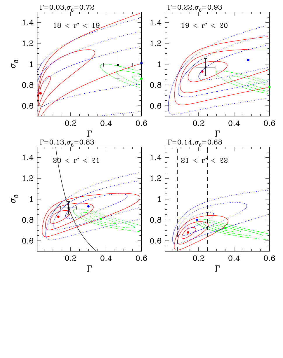
Figure 19.— Constraints on $\Gamma,\sigma_{8}$ using inverted power spectra in four magnitude bins. In each panel, red (solid lines) and blue (dotted lines) contours show the constraints using the power spectrum inverted from $w(\theta)$ and $C_{l}$ (restricted to scales $k<0.22$h Mpc^-1), respectively. Green contours (dot-dashed lines) show the constraints using all the $C_{l}$ measurements of T01. The solid square point with errorbars in the three bright magnitude bins is the best-fit parameter values and the black curve (solid line) in the $20<r^{*}<21$ magnitude bin is the constraint $\Gamma\sigma_{8}=0.173$, from the KL estimation technique of Sz01.

Figure 19 shows that the best-fit values of $\Gamma$ and $\sigma_{8}$ from $w(\theta)$ and $C_{l}$ are consistent with each other in all magnitude bins, with disagreements never exceeding about $1.5\sigma$ (recall that the joint 2D contours are broader than those shown). In the two intermediate magnitude bins, these best-fit values are also consistent with the maximum likelihood estimates using the KL technique from Sz01. It is reassuring that three different methods of estimating these power spectrum parameters, each of which makes different assumptions, yield consistent results. The contours from the $C_{l}$ measurements of T01 (green contours) appear inconsistent with all these three results. However, this appearence is illusory, a direct result of including all the $C_{l}$ measurements. Many of these are contaminated by non-linearities in the galaxy power spectrum. As discussed in §4.1, the observational window functions corresponding to $C_{l}$ are broad, extending to quite non-linear scales (see Fig. 5 of T01). Indeed, we find that by fitting the linear theory model power spectrum to the power spectrum inverted from $C_{l}$ on all scales (i.e. not restricting the analysis to $k<0.2\$h Mpc^-1), we can exactly reproduce the constraints from directly fitting to the $C_{l}$ measurements.

As can be seen from Figure 12, the power spectrum estimated from the faintest magnitude bin has a smaller amplitude and is less non-linear than the power spectrum in the brighter bins. Hence, we expect that the constraints on the shape parameter $\Gamma$ from this bin is least affected by non-linear evolution. Therefore, we adopt as our best estimate of $\Gamma$ the value obtained from inverting $w(\theta)$ in the $21<r^{\prime}<22$ magnitude bin. We estimate the error in $\Gamma$ by marginalizing over $\sigma_{8}$. Thus, our best estimate of $\Gamma$ is

$$\Gamma=0.14^{+0.11}_{-0.06},$$ (19)

where the error bars are derived by projecting the $\Delta\chi^{2}=4$ contour onto the $\Gamma$ axis, and therefore correspond to a $95\%$ confidence interval. This value of $\Gamma$ is consistent with the best-fit values of $\Gamma$ derived by Sz01 in the $20<r^{\prime}<21$ magnitude bin. It is also consistent with the value estimated by Percival et al. (2001), from the 2dFGRS (see the discussion in Sz01 for a detailed comparison the 2dFGRS results).

These results on inverting the 3D power spectrum from photometric galaxy catalogs bode well for the future. The inverted power spectrum using only the SDSS commissioning data already probes interestingly large scales. It is reasonable to expect that estimates of the power spectrum from all the galaxies expected in the entire SDSS photometric survey, which will be about fifty to a hundred times larger than this early catalog, will be among the most discriminating in cosmology.

Acknowledgements: The Sloan Digital Sky Survey (SDSS) is a joint project of The University of Chicago, Fermilab, the Institute for Advanced Study, the Japan Participation Group, The Johns Hopkins University, the Max-Planck-Institute for Astronomy (MPIA), the Max-Planck-Institute for Astrophysics (MPA), New Mexico State University, Princeton University, the United States Naval Observatory, and the University of Washington. Apache Point Observatory, site of the SDSS telescopes, is operated by the Astrophysical Research Consortium (ARC). Funding for the project has been provided by the Alfred P. Sloan Foundation, the SDSS member institutions, the National Aeronautics and Space Administration, the National Science Foundation, the U.S. Department of Energy, the Japanese Monbukagakusho, and the Max Planck Society. The SDSS Web site is http://www.sdss.org/.

SD and RS are supported by the DOE and by NASA grant NAG 5-7092 at Fermilab, and by NSF Grant PHY-0079251. MT is supported by NSF grant AST00-71213, NASA grant NAG5-9194 and the University of Pennsylvania Research Foundation.

References

- Bardeen et al. (1986) Bardeen, J., Bond, J. R., Kaiser, N., & Szalay, A. 1986, ApJ304, 15
- (2) Baugh, C. M. & Efstathiou, G. 1993, MNRAS 265, 145
- (3) Bond, J. R., Crittenden, R. G., Jaffe, A. H.& Knox, L. 1999, Computing in Science and Engineering, March-April 21
- (4) Budavari, T., Szalay, A.S., Connolly, A.J., Csabai, I. & Dickinson, M.E., AJ 20, 1588 (2000)
- (5) Connolly, A. J., Csabai, I., Szalay, A. S., Koo, D. C., Kron, R. G., & Munn, J. A. 1995, AJ 110, 2655
- (6) Connolly, A. J. et al., 2001 (C01)
- (7) Csabai, I., Connolly, A.J., Szalay, A.S. & Budavári, T. 2000, AJ 119, 69
- (8) Dodelson, S. & Gaztanaga, E. 2000, MNRAS 312, 774
- (9) Efstathiou, G. & Moody, S. J. 2000, astro-ph/0010478
- (10) Eisenstein, D. J. & Zaldarriaga, M. 2001, ApJ546, 2 (EZ)
- (11) Fernández-Soto, A., Lanzetta, K.M. & Yahil, A. 1999, ApJ513, 34
- (12) Fukugita, M., Shimasaku, K., & Ichikawa, T. 1995, PASP 107, 945
- (13) Fukugita, M., et al. 1996, AJ 111, 1748
- (14) Gunn, J. E. G. et al. 1998, AJ 116, 3040
- (15) Lilly, S.J., Le Fe’vre O., Crampton, D., Hammer, F., & Tresse, L. 1995, ApJ455, 50
- (16) Limber, D. N. 1953, ApJ 117, 134
- (17) Lin, H. et al. 1999, ApJ 518, 533 (CNOC2)
- (18) Lupton, R. H. et al. 2001, in ASP Conf. Ser. 238, Astronomical Data Analysis Software and Systems X, ed. F. R. Harnden Jr., F. A. Primini, and H. E. Payne (San Francisco: Astr. Spc. Pac.), in press (astro/ph/0101420)
- (19) Maddox, S. J., Sutherland, W. J., Efstathiou, G., & Loveday, J. 1990 MNRAS 242, 43p
- (20) Peebles, P. J. E. 1980, The Large-Scale Structure of the Universe (Princeton: Princeton University Press)
- (21) Percival, W. J., et al. 2001, submitted to MNRAS, astro-ph/0105252
- (22) Press, W. H., Teukolsky, S. A., Vetterling, W. T., & Flannery, B. P. 1992, Numerical Recipes (Cambridge: Cambridge University Press)
- (23) Sawicki, M.J., Lin, H. & Yee, H.K.C 1997, AJ113, 1
- (24) Scoccimarro, R. & Sheth, R. K. 2001, astro-ph/0106120
- (25) Scranton, R. & Dodelson, S. 2000, submitted to MNRAS, astro-ph/0003034
- (26) Scranton, R. et al. 2001 (Sc01)
- (27) Stoughton C., et al. 2001, submitted to AJ
- (28) Szalay, A. et al. 2001 (Sz01)
- (29) Tegmark, M., Hamilton, A. J. .S., Strauss, M. A., Vogeley, M. A., & Szalay, A. S. 1998, ApJ, 499, 555
- (30) Tegmark, M. et al 2001 (T01)
- (31) Yasuda, N. et al. 2001, ApJ, in press
- (32) York, D. G. et al. 2000, AJ120, 1579