Magnetic Helix Formation Driven by Keplerian Disk Rotation in an External Plasma Pressure — The Initial Expansion Stage

Abstract

We study the evolution of a magnetic arcade that is anchored to an accretion disk and is sheared by the differential rotation of a Keplerian disk. By including an extremely low external plasma pressure at large distances, we obtain a sequence of axisymmetric magnetostatic equilibria and show that there is a fundamental difference between field lines that are affected by the plasma pressure and those are not (i.e., force-free). Force-free fields, while being twisted by the differential rotation of the disk, expand outward at an angle of $\sim 60^{\circ}$ away from the rotation axis, consistent with the previous studies. These force-free field lines, however, are enclosed by the outer field lines which originate from small disk radii and come back to the disk at large radii. These outer fields experience most of the twist, and they are also affected most by the external plasma pressure. At large cylindrical radial distances, magnetic pressure and plasma pressure are comparable so that any further radial expansion of magnetic fields is prevented or slowed down greatly by this pressure. This hindrance to cylindrical radial expansion causes most of the added twist to be distributed on the ascending portion of the field lines, close to the rotation axis. Since these field lines are twisted most, the increasing ratio of the toroidal $B_{\phi}$ component to the poloidal component $B_{R,z}$ eventually results in the collimation of magnetic energy and flux around the rotation axis. We discuss the difficulty with adding a large number of twists within the limitations of the magnetostatic approximation.

Draft version

Subject headings: Accretion, Accretion Disks — Magnetic Fields – MHD — Plasmas

1 Introduction

The process of forming collimated jets/outflows due to disk accretion onto central compact objects is thought to depend on how magnetic fields behave when they are swirled around by the accretion disk. The progress of understanding this process has, however, been hindered by the significant lack of knowledge on the global magnetic field configuration in/near the accretion disk (see Okamoto 1999 for detailed critiques on many MHD models; see also Blandford 2000 for a recent review). An ordered magnetic field is widely thought to have an essential role in jet formation from a rotating accretion disk. Two main regimes have been considered in theoretical models (see Lovelace, Ustyugova & Koldoba 1999 for a review), the hydromagnetic regime where the energy and angular momentum is carried by both the electromagnetic field and the kinetic flux of matter, and the Poynting flux regime where the energy and angular momentum outflow from the disk is carried predominantly by the electromagnetic field. Major progress has been made recently in the hydromagnetic regime of jet formation, originally proposed by Blandford & Payne (1982). Dynamic MHD simulations of the near jet region have been carried out by several groups (Bell 1994; Ustyugova et al. 1995, 1999; Koldoba et al. 1995; Romanova et al. 1997, 1998; Meier et al. 1997; Ouyed & Pudritz 1997; Krasnopolsky, Li, & Blandford 1999). The simulation study of Ustyugova et al. (1999) in the hydromagnetic wind regime indicates that the outflows are accelerated to super-fast magnetosonic, super-escape speeds close to their region of origin ($\sim 80\times$ the inner radius of the disk), whereas the collimation occurs at much larger distances. Poynting flux models for the origin of jets were proposed by Lovelace (1976) and Blandford (1976) and developed further by Lovelace, Wang, and Sulkanen (1987), Lynden-Bell (1996), and Colgate & Li (1999). In these models the rotation of a Keplerian accretion disk twists a poloidal field threading the disk, and this results in outflows from the disk which carry angular momentum (in the twist of the field) and energy (in the Poynting flux) away from the disk, thereby facilitating the accretion of matter. Most recent computer simulations using the full axisymmetric MHD equations have been in the hydromagnetic regime. However, recent simulation studies have found jet outflows in the Poynting flux regime (Romanova et al. 1998; Ustyugova et al. 2000).

One class of models deals with a simplified limit, where magnetostatic and force-free conditions are assumed. This kind of problem is very clearly stated in the introduction of Lynden-Bell & Boily (1994, hereafter LB94; see also Lynden-Bell 1996): A field rooted in a heavy conductor on $z=0$ (i.e., the rotating disk) pervades a perfectly conducting force-free medium in the region $z>0$. On the disk surface ($z=0$), the field passes upwards from the region $0\leq R\leq R_{\rm o}$ and returns downwards in the region $R_{\rm o}<R\leq R_{\rm max}$. The disk is now rotated about its axis according to the Keplerian motion, $\Omega(R)\propto R^{-3/2}$. The problem is to determine the magnetostatic field configuration when the disk has gone through a specific number of turns. They found that fields, instead of collimating along the rotation axis, expand along an angle of $\theta\approx 60^{\circ}$ away from the rotation axis.

The behavior of twisted magnetic field lines that are anchored in a perfectly conducting medium has originally been considered in the solar corona context (see, e.g., Aly 1984, 1991, 1995; Mikic et al. 1988; Finn & Chen 1990; Sturrock et al. 1995). The direct application of those studies to accretion disks has been fairly recent (e.g., Appl & Camenzind 1993; Königl & Ruden 1993; LB94; Lynden-Bell 1996; Bardou & Heyvaerts 1996; Goodson et al. 1999; Uzdensky et al. 2000). The important role of an external plasma pressure was first emphasized by Lynden-Bell (1996) where he argued that field lines can not simply expand to infinity as shown by LB94 because the required $PdV$ work becomes too large. He then constructed a simplified cylindrical model where a magnetic helix/jet is bounded at large radius by external plasma pressure. But the question left open is whether the plasma pressure can indeed play a confining role in a self-consistent global treatment of the twisting and expansion of magnetic fields driven by the disk shear rotation.

In this study, we obtain self-consistent global solutions of axisymmetric magnetostatic configurations by strictly enforcing the Keplerian shear condition on the flux surfaces that are anchored in the disk. The assumptions we use are explained in detail in §2. We formulate our problem in §3, along with the relevant equations and methods to solve them. Results are given §4 and final conclusions and discussions are in §5.

2 Basic Assumptions

The equation of motion in the non-relativistic ideal magnetohydrodynamics (MHD) limit is simply

$$\rho\frac{d{\bf v}}{dt}=\frac{1}{c}~{}{\bf J\times B}+\rho{\bf g}-\nabla P~{},$$ (1)

where $\rho$ is the plasma density, ${\bf v}$ the flow velocity, ${\bf J}$ the current density, ${\bf g}$ the gravitational acceleration, and $P$ is the plasma pressure.

We restrict our attention to axisymmetric magnetostatic configurations. The underlying assumption is that the speed of the field line twisting by the disk is slow so that the system quickly reaches an equilibrium. We can then treat the evolution of field configurations as sequences of magnetostatic equilibria. We make the further assumption that the magnetic field plays the dominant role with plasma flow ${\bf v}$ and gravity $\rho{\bf g}$ much less important. Then, the steady state equation is

$${\bf J\times B}=c~{}\nabla P~{}~{}.$$ (2)

The main astrophysical motivation for keeping this pressure term is that at sufficiently large distances away from the disk, the plasma pressure will be comparable to the magnetic pressure, thus becoming dynamically important. When $\nabla P\rightarrow 0$, we have the so-called force-free (FF) limit.

We now discuss the physical conditions where these assumptions apply. There are at least two relevant speeds in this problem which are related to two physical aspects. The first one is the velocity of Keplerian disk rotation, $v_{\rm K}$, which describes the rate of field line footpoint movement. The second is the relaxation speed, $v_{\rm X}$, for magnetic fields to reach equilibrium, which is usually achieved by MHD waves going back and forth in the system. This is essentially the Alfvén speed $v_{\rm A}$ and is ultimately limited by the speed of light $c$. Together with these speeds, there are two relevant timescales: the disk rotation period $T_{\rm K}=2\pi R_{\rm min}/v_{\rm K}$, and the relaxation time $T_{\rm X}=L_{\rm max}/v_{\rm X}$, where $R_{\rm min}$ is the inner disk radius, and $L_{\rm max}$ the system dimension, respectively. In order to ensure the steady state condition on the timescale of $T_{\rm K}$, one requires that $L_{\rm max}\ll(v_{\rm X}/v_{\rm K})R_{\rm min}$.

In order to simulate a system that is much larger than $R_{\rm min}$, these considerations indicate that in a black hole accretion disk system, field lines close to the black holes are likely twisted too rapidly to be treated by the magnetostatic equations. In other words, the dynamic pressure from the inertial term $\rho d{\bf v}/dt$ in equation (1) is likely to be very important during the expansion, thus the conclusions from this study might not apply in this limit. On the other hand, for field lines further away from the black hole and/or for accretion disks around systems like young stars, the rotation speed is small enough that the magnetostatic limit could still apply.

Another relevant process is the footpoint drift across the disk. Magnetic field threading the disk tends to be advected inward with the accretion flow, but at the same time it may diffuse through the disk owing to a finite magnetic diffusivity $\eta_{m}$ of the disk. The outward drift of the magnetic field in the disk occurs at speed ${\cal U}_{r}=(\eta_{m}/h)\tan(\theta)$, where $h$ is the half-thickness of the disk, $\tan(\theta)\equiv(B_{r}/B_{z})_{z=0}$, and a smaller, second order diffusion term ($\eta_{m}\partial^{2}B_{z}/\partial r^{2}$) has been omitted (Lovelace et al. 1997). For cases where the diffusivity is of the order of the viscosity and where the viscosity is given by the Shakura and Sunyaev (1973) prescription $\nu=\alpha c_{s}h$ (with $\alpha<1$ and $c_{s}$ the midplane sound speed), the diffusive drift speed is ${\cal U}_{r}\sim\alpha c_{s}\tan(\theta)$. This is larger than the radial accretion speed $v_{r}\sim-\alpha c_{s}(h/R)$ due to viscosity alone. But what is important here is that the field drift and the accretion speeds are much less than the Keplerian velocity of the disk for $c_{s}\ll V_{K}$. For this reason the fields can be treated as frozen into the disk. This point was made by Ustyugova et al. (2000) and also discussed by Uzdensky et al. (2000).

3 Basic Equations

We have formulated the problem discussed in §1 in both cylindrical $(R,\phi,z)$ and spherical $(r,\theta,\phi)$ coordinates. Axisymmetry is assumed in both cases. The magnetic field can be written as:

$${\bf B}={\bf B}_{p}+B_{\phi}\hat{\bf\phi}=\nabla\Psi\times\nabla\phi+B_{\phi}\hat{\bf\phi}~{},$$ (3)

where the poloidal component ${\bf B}_{p}$ is in the $\{R,z\}$ or $\{r,\theta\}$ plane, $2\pi\Psi$ is the total poloidal flux through the disk, and contours of $\Psi$ label the poloidal field lines. The poloidal magnetic fields are

$$B_{R}=-{1\over R}{\partial\Psi\over\partial z}~{},\quad B_{z}={1\over R}{\partial\Psi\over\partial R}~{},$$ (4)

for cylindrical coordinates and

$$B_{r}={1\over r^{2}\sin\theta}{\partial\Psi\over\partial\theta}~{},\quad B_{\theta}=-{1\over r\sin\theta}{\partial\Psi\over\partial r}~{},$$ (5)

for spherical coordinates. The current density

$$\frac{4\pi}{c}{\bf J}=-\Delta^{\star}\Psi\nabla\phi+\nabla(rB_{\phi})\times\nabla\phi~{},$$ (6)

where the operator $\Delta^{\star}$ is, for cylindrical coordinates,

$$\Delta_{c}^{\star}\Psi=\frac{\partial^{2}}{\partial R^{2}}-\frac{1}{R}\frac{\partial}{\partial R}+\frac{\partial^{2}}{\partial z^{2}}~{},$$ (7)

and for spherical coordinates,

$$\Delta_{s}^{\star}\Psi=\frac{\partial^{2}}{\partial r^{2}}+\frac{1}{r^{2}}\frac{\partial^{2}}{\partial\theta^{2}}-\frac{1}{r^{2}\tan\theta}\frac{\partial}{\partial\theta}~{}.$$ (8)

Equation (2) implies that

$${\bf B}\cdot\nabla P=0~{}~{}\Longrightarrow~{}~{}P=P(\Psi)~{}.$$ (9)

In other words, the gas pressure is constant along field lines. In cylindrical coordinates, equation (2) can be written as the well-known Grad-Shafranov equation,

$$\Delta_{c}^{\star}\Psi\nabla\Psi+RB_{\phi}\nabla(RB_{\phi})=-4\pi R^{2}\frac{dP}{d\Psi}\nabla\Psi~{},$$ (10)

from which we define $RB_{\phi}=H(\Psi)$ and we get

$$\Delta_{c}^{\star}\Psi+d[H^{2}/2]/d\Psi+4\pi R^{2}dP/d\Psi=0~{}.$$ (11)

Similarly, in spherical coordinates, we define $r\sin\theta B_{\phi}=H(\Psi)$ and

$$\Delta_{s}^{\star}\Psi+d[H^{2}/2]/d\Psi+4\pi(r\sin\theta)^{2}dP/d\Psi=0~{}.$$ (12)

In our spherical calculations, we actually use $\xi=\ln r$ to concentrate the uniform grid in $\xi$ for better resolution at small $r$. Equation (12) then becomes

$$\Delta_{sl}^{\star}\Psi+r^{2}d[H^{2}/2]/d\Psi+4\pi(r^{4}\sin\theta^{2})dP/d\Psi=0~{},$$ (13)

where

$$\Delta_{sl}^{\star}\Psi=\frac{\partial^{2}}{\partial\xi^{2}}-\frac{\partial}{\partial\xi}+\frac{\partial^{2}}{\partial\theta^{2}}-\frac{1}{\tan\theta}\frac{\partial}{\partial\theta}~{}.$$ (14)

The quantity $H(\Psi)=RB_{\phi}(R,z)$ is $(2/c)$ times the total current flowing through a circular area of radius $R$ (with normal $\hat{\bf z}$) labeled by $\Psi(R,z)$= const. The development of the toroidal field component from an initial purely poloidal field comes from the differential rotation of the disk onto which footpoints of the same field lines are anchored.

3.1 Boundary Conditions

Since there is no direct observational information on how magnetic fields are distributed on the surface of an accretion disk, we have made the following assumptions. If the magnetic fields on the disk is initially generated via an accretion disk dynamo that makes a quadrupole or dipole-like field, magnetic fields will emerge out of the disk at smaller radii and go back to the disk at large radii. We use $R_{\rm o}$ to represent the O-point of the field in the disk, i.e., the radius where $B_{z}=0$ on the disk. Furthermore, in a fully self-consistent treatment including the back-reaction on the disk, $R_{\rm o}$ also marks a separation location inside which angular momentum is lost and transmitted to the outer part of the disk by field line tension.

We study the expansion of this cylindrical magnetic arcade anchored on the disk. We further assume that the overall strength of $|B_{z}|$ decreases as a function of radius, except near the O-point where $|B_{z}|=0$. This is roughly consistent with the fact that the thermal pressure of the disk (which anchors the fields) decreases radially as well. Specifically, we have chosen a computational domain that is a box with $0<R<R_{\rm max}$ and $0<z<z_{\rm max}$ in the cylindrical case and/or a sphere with $r_{\rm min}<r<r_{\rm max}$ in the spherical case. The outer boundary is assumed to be perfectly conducting ($\Psi=0$). At $z=0$ (along the disk), we assume that the disk is perfectly conducting as well. An initial poloidal field distribution is specified $\Psi(R,0)$ [or $\Psi(r,\pi/2)$] as

$$\Psi(R,0)\propto\cases{R^{2}&for $R<R_{c}$ ;\cr R^{\alpha}&for $R_{c}<R<R_{\rm o}$;\cr R_{\rm out}^{\alpha}-R^{\alpha}&for $R_{\rm o}<R<R_{\rm out}$,\cr}$$ (15)

where we have joined these parts smoothly. Figure 1 shows the distribution of $\Psi$ and $|B_{z}|$ on the disk surface. The poloidal flux is distributed between $R_{\rm min}\approx 10^{-5}$ and $R_{\rm out}\approx 0.02$. A core radius $R_{c}\approx 10R_{\rm min}$ is used, inside of which the $B_{z}$ component approaches a constant. The index $\alpha$ is chosen to be $5/4$, so that $B_{z}$ is decreasing as $R^{\alpha-2}$, reversing its sign at the O-point $R_{\rm o}\approx 0.01$, and continuing decreasing until $R_{\rm out}$. Both $\Psi(R,0)$ and $|B_{z}|$ remain zero between $R_{\rm out}$ and $R_{\rm max}=1$. These choices for $R_{\rm o}$ and $R_{\rm out}$ ensure that the initial magnetic field is distributed far inside the outer boundary $R_{\rm max}$. We have tried many different initial field configurations and found that our main conclusions do not depend on these particular choices of parameters, as long as magnetic fields stay away from the outer boundary $R_{\rm max}$ or $r_{\rm max}$. The dependence on $\Psi(R,z=0)$ near the O-point is very weak since those field lines are hardly twisted at all.

3.2 External Plasma Pressure

The physical picture we have in mind for accounting for the pressure of an external plasma is that magnetic field close to the disk is force-free with little influence from the plasma pressure. At large distances, however, the magnetic pressure decreases sufficiently so that plasma pressure becomes important. In other words, the magnetic fields are bounded above and on the sides by an ambient medium which is perfectly conducting and mostly devoid of any magnetic flux. This forms a conducting, in general, “deformed box” inside of which the magnetic field dominates and the gas pressure is very small.

To model the external plasma pressure, we adopt the dependence

$$P(\Psi)=P_{c}\exp[-(\Psi/\Psi_{c})^{2}]~{},$$ (16)

so that

$$dP/d\Psi=-(2P_{c}/\Psi_{c}^{2})~{}\Psi~{}\exp[-(\Psi/\Psi_{c})^{2}]~{},$$ (17)

where $P_{c}$ and $\Psi_{c}$ are the input parameters. For most of the results presented here, we have chosen $P_{c}=0.1$ and $\Psi_{c}=10^{-3}$. The physical meaning of $P_{c}$ is that its magnitude gives an estimate of the overall importance of plasma pressure. Using the example given in equation (15), the maximum $B_{z}$ near $R_{\rm min}$ is $\sim 6\times 10^{5}$, (see Figure 1), so the ratio of the maximum magnetic pressure to the maximum gas pressure in the computational domain is $\sim 10^{11}$. The quantity $\Psi_{c}$ gives the fraction of poloidal flux that is affected by the plasma pressure.

The prescribed plasma pressure (equation 16) is kept fixed at all times throughout the sequence of equilibria. This is because the prescribed pressure here is meant to mimic a constant external pressure boundary (such as pressure from interstellar or intergalactic medium) that is reacting to the “push” by magnetic fields. This interpretation is precise in the limit of $\Psi_{c}\rightarrow 0$. We have used a very small but finite $\Psi_{c}$ for the convenience of modeling both the Lorentz force and pressure gradient terms simultaneously, rather than having to specify the pressure gradient term through a boundary condition, especially when the shape of this boundary is determined dynamically by the push from the magnetic fields and is not known a priori. The pressure in the flux tubes with $\Psi>\Psi_{c}$, however, might change due to the flux volume expansion. If the entropy of each flux tube is conserved, then pressure has to decrease with expanding volume. On the other hand, if there is enough heat flux between the disk and the flux tubes, then the entropy of a flux tube is not conserved (Finn & Chen 1990). Either way, since the pressure in the flux tubes with $\Psi>\Psi_{c}$ is already set to be exponentially small (equation 16) initially, any further decrease in pressure will not alter our conclusions.

We make two more observations about the plasma pressure term. First, equation (16) gives that, when $\Psi\rightarrow 0$ (i.e., at the boundary), the pressure $P\rightarrow P_{c}$ and its gradient $dP/d\Psi\rightarrow 0$. Both features are physically plausible. Second, it is interesting to note that the pressure effect enters equations (11) and (13) with a geometric factor $R^{2}$ or $(r\sin\theta)^{2}$. This factor actually comes from the ${\bf J\times B}$ term. It is only under the equilibrium condition can it be “moved” to be a multiplier of the pressure term. Consequently, the pressure tends to prevent expansion away from the rotation axis but has relatively little constraining effect along the rotation axis.

3.3 Input Keplerian Field Line Twist

From the distribution of $\Psi(R,0)$ and the Keplerian rotation $\Omega(R)\propto R^{-3/2}$, we can define the required twist on each field line $\Delta\Phi(\Psi)$. The twist of a given field line going from an inner footpoint at $R_{1}$ to an outer footpoint at $R_{2}$ is proportional to the differential rotation of the disk. Using a cylindrical coordinate, for a given field line, we have

$$Rd\phi/B_{\phi}=d\ell_{p}/B_{p}~{},$$

where $d\ell_{p}\equiv\sqrt{dR^{2}+dz^{2}}$ is the poloidal arc length along the field line, and $B_{p}\equiv\sqrt{B_{R}^{2}+B_{z}^{2}}$. Then the total twist of a field line is

$$\Delta\Phi(\Psi)=\int_{1}^{2}d\ell_{p}~{}{B_{\phi}\over RB_{p}}=H(\Psi)\int_{1}^{2}{d\ell_{p}\over R^{2}B_{p}}~{}.$$ (18)

We denote the quantity $V^{\prime}(\Psi)=\int_{1}^{2}d\ell_{p}/R^{2}B_{p}$. The field line twist after a time $t$ is

$$\Delta\Phi(\Psi) = \Omega_{o}~{}t\left[\left({R_{\rm o}\over R_{1}}\right)^{3/2}-\left({R_{\rm o}\over R_{2}}\right)^{3/2}\right]~{},$$ (19)

$$= (\Omega_{o}~{}t)~{}{\cal F}(\Psi)$$

where $\Omega_{o}\equiv\sqrt{GM/R_{\rm o}^{3}}$ is the Keplerian angular frequency at $R_{\rm o}$ of an object of mass $M$, and ${\cal F}$ is dimensionless. The rotation profile is assumed to begin deviating from Keplerian and approach a constant when $R\leq R_{\rm c}$ (the bottom panel of Figure 1). There exists a region, however, between $\Psi=0$ and $\Psi_{\rm min}=\Psi(R_{\rm min})$ where the twist decreases as $\Psi$ decreases (i.e., getting closer to the $z$-axis and the surrounding wall). These field lines are not explicitly followed in our calculations. But since $H(\Psi)\rightarrow 0$ as $\Psi\rightarrow 0$, the twist $\Delta\Phi(\Psi)$ approaches zero as well [equation (18)].

3.4 Method of Solution

We solve equations (11) and (13) following the approach given in Finn & Chen (1990), which employs several levels of iterations. For the very first step, we will use a trial $H(\Psi)$, then we solve equation (11) or (13) using the Successive Over-Relaxation (SOR) method (see for example, Potter 1973) for $\Psi^{k}(r,\theta)\rightarrow\Psi^{k+1}(r,\theta)$. From $\Psi^{k+1}(r,\theta)$, we integrate along the field lines to obtain $V^{\prime}(\Psi)$. We typically trace $\sim 200$ field lines with $3\times 10^{-5}\leq\Psi\leq 1$ for calculating the poloidal current profile $H(\Psi)$. Using equation (18), we update $H(\Psi)$ using the input $\Delta\Phi(\Psi)$. This procedure is then repeated. The advantage of the simple SOR solver is that the nonlinear source terms $d(H^{2})/d\Psi$ and $dP/d\Psi$ can be easily included in the iterations so that convergence can be achieved fairly quickly (with a typical relative residue less than $10^{-6}$)

In summary, we compute global magnetostatic solutions of $\Psi(r,\theta)$ using the Grad-Shafranov equation in axisymmetry by requiring that the twist on each field line follows a specified function $\Delta\Phi(\Psi)$, derived based on the Keplerian disk rotation.

4 Results

We have made many runs with different choices of the initial field configuration on the disk $\Psi(R,0)$, the twist profile $\Delta\Phi(\Psi)$, and the pressure profile $P(\Psi)$. Runs are made in both cylindrical and spherical coordinates. We present most of our results using the following parameters: A $\ln r-$spherical coordinate system is used, with $r_{\rm min}=10^{-5},r_{\rm max}=1$. The radial and $\theta-$angle grids are $367\times 51$. The initial field configuration is the same as shown in Figure 1, where $R_{\rm o}=0.01$ and $R_{\rm out}=0.02$. The smallest $\Psi$ value of the field lines we track is $\Psi_{\rm min}=\Psi(R_{\rm min})=3\times 10^{-5}$. The plasma pressure parameters are $P_{c}=0.1$ and $\Psi_{c}=0.001$. The maximum $|B_{z}|$ on the disk is $\approx 6\times 10^{5}$, which implies a ratio of $\sim 10^{11}$ between the maximum magnetic pressure and the plasma pressure. (Even larger pressure ratios can be achieved with relative ease.) To indicate the progressively increasing twist added to the field lines, we use the notation time “$t$” [equation (19)] in units of revolutions of the inner most flux line ($\Psi_{\rm min}$) around the $z$-axis, i.e., $\Delta\Phi_{\rm max}=\Delta\Phi(\Psi_{\rm min})=2\pi t$.

Figure 2 describes our overall physical picture with two different physical regimes. For $0\leq\Psi\leq\Psi_{c}$, the plasma pressure is dominant. This region is labeled as “plasma-pressure” (PP). For $\Psi_{c}\leq\Psi\leq 1$, the magnetic pressure dominates, the region is force-free (labeled as “FF”). So, we have effectively made two ideal MHD fluids, one (PP) has a plasma $\beta\rightarrow\infty$ and the other (FF) has $\beta=0$. The key question we are addressing is: “how does the shape of $\Psi=\Psi_{c}$ boundary change while field lines are being twisted by the Keplerian disk rotation?” In other words, the boundary between the PP and FF regions evolves according to both the expansion and “pushing” from the FF region and the “hindrance” of the plasma pressure.

Although some details may differ, we generally find that magnetic fields evolve in the following manner: (1) in the FF region, field lines expand primarily towards the large radius along an angle (from the $z$-axis) of $\theta\sim 45^{\circ}-60^{\circ}$; (2) in the PP region, field lines expand predominantly vertically (along the $z$-axis) with some slight radial expansion; (3) more twist causes further expansion along the $z$-axis but subject to a break-down of the magnetostatic, equilibrium assumption. We now discuss these features in detail.

4.1 Equilibrium Sequence with Increasing Twist

Figure 3 shows the evolution of magnetic fields in the poloidal plane as twist is added, with $t=0,1,2$ and $4$ turns, respectively. The field lines shown are evenly spaced in $\log_{10}(\Psi)$, with the outer-most line having $\Psi\approx 10^{-4}$ and the inner-most line having $\Psi\approx 0.5$. Here, we use the term “outer” to refer to field lines in the PP region, which originate from the smallest radii and return back to disk at the largest radii. The term “inner” refers to field lines around the O-point in the FF region. Consequently, because the field lines are twisted according to the Keplerian rotation (largest rotation at the smallest radius), the outer field lines show substantial “movement” due to the added twist, whereas field lines around the O-point show little change.

The corresponding results for the poloidal current $H(\Psi)$ and the resultant twist $\Delta\Phi$ are plotted in Figure 4. It is interesting to note that $H(\Psi)$ can be approximated by two power-laws of $\Psi$, where $H(\Psi)\propto\Psi$ when $\Psi\leq\Psi_{c}$ and flattens somewhat for $\Psi>\Psi_{c}$. The twist shown in the lower panel is derived by integrating along each field line. They indeed follow closely the input profile due to Keplerian rotation.

4.2 Role of External Plasma Pressure in Collimation

The striking feature of the sequence of equilibria in Figure 3 is the way the outer field lines expand. To best understand this behavior, we separate the field lines into two groups according to the ratio of $\Psi/\Psi_{c}$. These two groups have fundamentally different expansion behavior, which is illustrated in Figure 5, where the expansion of three different field lines ($\Psi=10^{-2},10^{-3},10^{-4}$) is shown for $t=0$ (solid), $t=2$ (dotted), and $t=4$ (dashed), respectively.

Field line expansion in the FF region has been studied in detail in many previous studies (see Introduction). The Lorentz force is the only force available (i.e., the magnetic pressure gradient is balanced by the tension force). As found for example by LB94, the field lines expand to large radii along an angle of $\theta\approx 60^{\circ}$ from the $z-$axis. This is consistent with the left panel of Figure 5 (also the inner field lines in Figure 3).

The field line expansion in the PP region, however, is fundamentally different from the FF regime. This is because the magnetic pressure becomes very small at large radii and eventually at some distance it becomes comparable to the surrounding plasma pressure. At this location, further expansion of the magnetic fields is greatly hindered by the plasma pressure. At the same time, increasing the twist acts to increase the ratio of $B_{\phi}/B_{R}$. Consequently, these field lines are increasingly “pinched” around the $z$-axis, and they eventually expand along the $z$-axis in a “collimated” fashion, as shown by the middle and right panels of Figure 5 and the late time in Figure 3.

The middle panel of Figure 5 is particularly important. It shows how the critical boundary at $\Psi=\Psi_{c}$ (see Figure 2) evolves with increasing twist. Note that its initial shape is quasi-spherical, but a clear collimation along the $z-$axis has developed by $t=4$.

A small amount of poloidal flux (with $\Psi<\Psi_{c}$) is in the PP region and is twisted as well. One can ask whether these outer field lines have contributed importantly to forming the new shape of the $\Psi=\Psi_{c}$ boundary. To answer this question, we have performed runs with a very small $\Delta\Phi(\Psi)$ for $\Psi<\Psi_{c}$, instead of the near constant $\Delta\Phi(\Psi)$ presented in Figure 4. We find that as long as $\Delta\Phi(\Psi_{c})$ remains the same, its shape does not depend on the twist profile for $\Psi<\Psi_{c}$. This means that the small amount of magnetic flux beyond the $\Psi=\Psi_{c}$ boundary does not change our results noticeably.

We have also performed runs with various magnitudes of the plasma pressure. For the purely force-free case, we confirm the results by LB94 that the field lines expand to large radii along an angle of $\theta\approx 60^{\circ}$ from the $z-$axis and only a small total twist (less than half a turn) can be added before the fields are packed against the outer boundary. With a finite pressure, however, the collimation effect is always observed as long as the simulation region is large enough or the pressure is large enough so that magnetic fields are not directly packed against the outer boundary.

Thus, the external plasma pressure, no matter how small it may be, plays a fundamental role in causing the field lines to collimate along the rotation axis. It essentially stops (or greatly slows down) the radial expansion of the field lines, and in the meantime allows the build-up of the toroidal component. This interpretation is also consistent with the fact that field lines are closely packed at large radius (stopped by plasma pressure) but are loosely spaced along the $z$-axis (see the “$t=4$” panel in Figure 3).

The results shown in Figures 3 and 5 indicate that the solution suggested by Lynden-Bell (1996) is indeed possible (at least in the early expansion stage of the helix formation), even though details are different. Here, we have shown global self-consistent solutions where the field lines are twisted according to the disk Keplerian rotation.

4.3 Distribution of Twist and Magnetic Energy

Figure 6 shows how its twist ($\Delta\phi$) is distributed along this field line as a function of $z$ at $t=4$. We have plotted another field line with a larger $\Psi_{2}=10^{-2}$ at $t=4$ as well. There is an important difference between these two field lines in the distribution of the twist $\Delta\Phi(\Psi)$. For $\Psi_{1}$, most of its twist ($\geq 75\%$) is distributed on the ascending portion of the field line and near the $z$-axis; the rest is distributed while the field line spirals down back to the disk. For $\Psi_{2}$, however, the twist is distributed uniformly between ascending and descending portions. To understand this difference, we can write

$$\left|\frac{d\phi}{dz}\right|=\left|\frac{RB_{\phi}}{R^{2}B_{z}}\right|=\left|\frac{H(\Psi)}{R\partial\Psi/\partial R}\right|~{}.$$

Note that $H(\Psi)$ is constant along a field line. Imagine a small flux tube ($\Psi\rightarrow\Psi+d\Psi$) originating from the inner region of the disk. Since the field line remains at small $R$ for the ascending section in the presence of plasma pressure, $B_{z}R^{2}\sim 2\Psi$. This is the reason why $d\phi/dz$ following a flux tube is roughly constant for the ascending part of the flux tube. For the $\Psi_{1}$ flux tube, however, its expansion at large radius (the descending portion) is strongly constrained by the plasma pressure, so that the cross section area for the descending flux tube is much smaller than it would have been without the plasma pressure. Consequently, its $B_{z}$ component on the descending portion of the $\Psi=\Psi_{1}$ surface varies more slowly than $R^{-2}$, so that the rate $|d\phi/dz|$ is smaller. Overall, the twist is then non-uniformly distributed on a flux line. (See Ch .9 of Parker 1979). Thus, the presence of plasma pressure leads to a strong collimation and a concentration of the twist to the collimated region.

The total injected toroidal flux ${\cal F}_{\phi}$ by the disk rotation into the system can be evaluated as

$${\cal F}_{\phi}(t)=\int\int B_{\phi}dRdz=\int_{0}^{1}d\Psi\Delta\Phi(\Psi,t)~{}.$$ (20)

We find that the ratio of ${\cal F}_{\phi}$ to the initial total poloidal flux, ${\cal F}_{z}=\int_{0}^{R_{\rm o}}dR2\pi RB_{z}=2\pi$, increases linearly with time as expected by equation (19), reaching a maximum of $\sim 4\%$ when $t=4$. So, the total injected toroidal flux is still a small fraction of the total initial poloidal flux. This information is useful for non-axisymmetric stability considerations for future studies.

Figure 7 shows the spatial distribution of magnetic energy density and how it evolves with added twist. The quantity $\log_{10}(B^{2}/P_{c}+1)$ (i.e., a scaled magnetic energy density) is shown for $t=0$ (top left) and $4$ (top right), where $B^{2}=B_{p}^{2}+B_{\phi}^{2}$ and $P_{c}=0.1$. It is clear that essentially all the magnetic energy is enclosed by the plasma pressure. The expansion results in a clear collimation of magnetic energy along the $z-$axis. The two bottom panels show, at $t=4$, the poloidal $\log_{10}(B_{p}^{2}/P_{c}+1)$ (lower left) and the toroidal $\log_{10}(B_{\phi}^{2}/P_{c}+1)$ (lower right) components, respectively. Note the dramatic increase of magnetic energy (mostly poloidal component) along the $z-$axis.

4.4 Limitation on Increase of Twist

We find that it is not possible to increase the twist beyond what is shown in Figure 3. When more twist is added, the system evolves from a configuration with all field lines being tied to the disk to a new topology with some poloidal field lines close on themselves instead of connecting to the disk (i.e., forming an isolated “island” of poloidal fluxes or “plasmoid”). At this point, our method used to solve equation (13) becomes unstable. The plasmoid formation is associated with the field lines that are in the FF regime ($\Psi>\Psi_{c}$). The transition to the plasmoid formation is sudden, giving a sense of eruptive behavior of the solution. However, as discussed below, this numerical behavior is associated with instability of the method but not necessarily related to instability of the MHD equations.

Such eruptive behavior has been the subject of intense research in the solar flare community (Aly 1984, 1991, 1995; Sturrock et al. 1995). The formation of a plasmoid from a single arcade (Inhester et al. 1992) is a loss-of-equilibrium bifurcation related to tearing instability of the current sheet which forms at the center of the arcade when it is sheared strongly (Finn et al. 1993). In addition, it has been shown that plasmoid formation can occur directly as a consequence of linear instability when multiple arcades exist (Mikic et al. 1988; Biskamp et a., 1989; Finn et al. 1992).

This behavior of the solutions with increasing twist can be traced to a mathematical nature of the elliptical equation we are solving (e.g., equation (11) and (13)). We can write this equation in a pseudo-time-dependent form, e.g.,

$$\frac{\partial\Psi}{\partial t}=\Delta^{\star}\Psi+\frac{1}{2}\frac{dH^{2}}{d\Psi}-AR^{2}\Psi\exp[-(\Psi/\Psi_{c})^{2}]~{},$$ (21)

where a steady state is achieved progressively when $\partial\Psi/\partial t\rightarrow 0$. Here, $A=8\pi P_{c}/\Psi_{c}^{2}$ is a positive constant. The computational domain can then be divided into three parts depending on the ratio of $\Psi/\Psi_{c}$. Region I: large $R$. The pressure term “$-R^{2}|dP/d\Psi|$” dominates. Since it is negative, it drives $\Psi$ to $0$ exponentially for small $\Psi$ (i.e., $d\Psi/dt\propto-C_{1}\Psi$, with $C_{1}>0$). The solution in this region is quite stable. Region II: small $R$ and small $z$ (close to the disk), i.e., the FF region with a negligible pressure term. Region III: small $R$ but large $z$ (along the rotation axis), where all three terms contribute. The eruptive behavior we found could occur in both regions II and III, whenever the poloidal current term $dH^{2}/d\Psi$ exceeds a certain critical value. With a large current, magnetic fields tend to expand enormously and fill up the whole computational domain.

An important question is whether this eruptive behavior actually occurs in a system described with the full set of dynamical equations. Recent axisymmetric simulations using the full set of MHD equations by Ustyugova et al. (2000) and Goodson et al. (1999) indicate that field lines can reconnect and become open. Clearly, the rate of reconnection is enhanced by the artificially large resistivity in such codes; the exact role of resistivity in allowing reconnection when it might not otherwise occur is not completely clear. In Ustyugova et al. (2000), two regimes have been found after $\sim$ tens of rotation periods of the inner disk: a hydromagnetic outflow from the outer part of the disk, and a Poynting outflow, which has negligible mass flux but is dominated by the electromagnetic field along the rotation axis.

5 Discussions and Conclusions

We have shown that a static plasma pressure is fundamental in shaping the overall magnetic equilibrium, despite the fact that the plasma pressure is exceedingly small (the maximum magnetic pressure over the plasma pressure is $10^{11}$ in this study). This is essentially different from the pure force-free models (e.g., LB94; see however Lynden-Bell 1996). This difference comes from the fact that the field lines that are being twisted the most expand the furthest so that they are most affected by the plasma pressure. This is opposite to the behavior in the solar flare models where most of the shear is concentrated around the O-point. The least amount of shear is applied near the O-point in the accretion disk case. In regions where the plasma pressure is negligible, the physics of expansion is dominated by the force-free condition (${\bf J\times B}=0$). Their expansion is predominantly towards larger radii along an angle of $\theta\sim 60^{\circ}$ from the $z-$axis (LB94). But for field lines affected by the plasma pressure, their radial expansion (away from the $z-$axis) is slowed or stopped by this pressure. The twisting of those field lines causes them to expand much more strongly along the $z-$axis due to the build-up of the toroidal field component $B_{\phi}$. The build-up of $B_{\phi}$ is non-uniform along those field lines, with more twist distributed on the ascending portion of the field lines. This is, again, a direct result of external plasma pressure.

We have obtained magnetostatic equilibria up to a maximum of $4$ turns of the inner most field line. For larger twist the solutions exhibit a change of topology and our method breaks down. The larger values of twist should be treatable by including the inertia term $\rho d{\bf v}/dt$ in the full set of dynamic MHD equation.

An important question is the stability/instability of these axisymmetric equilibria. Instabilities in 3D involving flux conversion between toroidal and poloidal components is probably unavoidable and this effect will be important astrophysically: this is because the initial poloidal flux on the disk is probably too small to be responsible for the observed total magnetic flux in many astrophysical systems (Colgate & Li 2000). The flux multiplication by the disk rotation/twisting, and subsequent flux conversion, could however generate enough flux.

We acknowledge many useful discussions with Drs. R. Kulsrud, M. Romanova, R. Rosner, and P. Sturrock. We thank an anonymous referee whose insightful comments have helped both in the clarification of the basic assumptions and the overall presentation of the paper. Part of this work was presented at an Aspen summer workshop on Astrophysical Dynamos in 2000. This research was performed under the auspices of the U.S. Department of Energy, and was supported in part by an IGPP/Los Alamos grant and the Laboratory Directed Research and Development Program at Los Alamos. RVEL was supported in part by NASA grants NAG5-9047 and NAG59735 and by NSF grant AST-9986936.

  Fig. 1.—: The distribution of poloidal fields on the disk between $0\leq R\leq R_{\rm out}$. Its $\Psi$ value is shown in the top panel, which increases from 0 to 1 at the O-point $R_{\rm o}=0.01$ and decreases back to 0 at $R_{\rm out}=0.02$. Its corresponding $|B_{z}(R,0)|$ is shown in the middle panel, where it becomes zero as well as reverses its sign at $R_{\rm o}$. The twist profile ($\propto R^{-3/2}$ is shown in the bottom panel. It is nearly Keplerian over large range of radii, but is flattened for $R\rightarrow 0$ and is approaching zero near the O-point because the separation between the footpoints of the arcade is becoming zero.

  Fig. 2.—: The overall physical picture with two different regimes, separated by $\Psi=\Psi_{c}$ (the thick dashed line). The region labeled “plasma-pressure” (PP) is dominated by the plasma pressure with $\Psi_{c}\geq\Psi\geq 0$ (the boundary at $r=1$). A tiny fraction (=$\Psi_{c}$) of the total poloidal flux is in this region. The region labeled “force-free” (FF) is dominated by the magnetic pressure with $\Psi_{c}\leq\Psi\leq 1$ (the O-point). Most of the poloidal flux ($1-\Psi_{c}$) is contained in this region. The key question we are addressing is the response of the $\Psi=\Psi_{c}$ boundary to the twisting of field lines by the Keplerian disk.

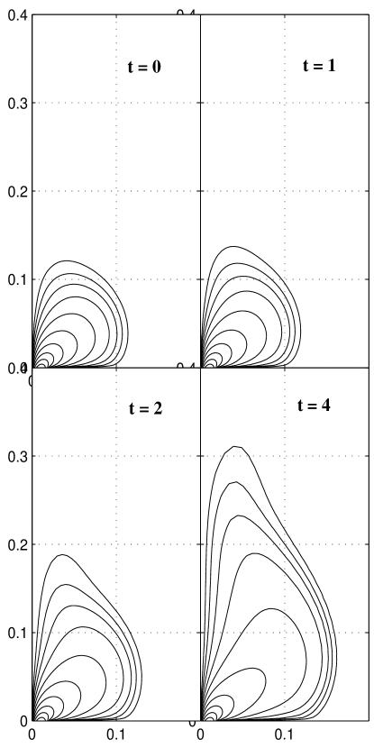
  Fig. 3.—: The “evolution” of the poloidal field lines with increasing twist as solutions of equation (13) in a $\ln r-$spherical coordinate for $t=0,1,2$ and $4$, respectively. (We present the results in a smaller $R-z$ plane for clarity.) The contours are displayed evenly in logarithmically spaced intervals ($10^{-4}\leq\Psi\leq 1$). The outer field lines have expanded more strongly along the $z-$axis (from $z\approx 0.1$ to $0.3$) than in the radial direction(from $R\approx 0.1$ to $0.15$).

  Fig. 4.—: The poloidal current $H(\Psi)$ (upper panel) and the twist $\Delta\Phi(\Psi)$ (lower panel) as a function of $\Psi$ for $t=1,2,4$, (bottom to top curves), respectively, for the run shown in Figure 3. The function $H(\Psi)$ is $\propto\Psi$ for small $\Psi$ then flattens as $\Psi$ increases. The twist agrees with the input Keplerian profile nearly perfectly with indistinguishable differences.

  Fig. 5.—: The “movement” of three particular poloidal field lines, $\Psi=10^{-2}$ (left), $10^{-3}$ (middle), and $10^{-4}$ (right), as their twist increases from $t=0$ (solid), $2$ (dotted) to $4$ (dashed), using the results from Figure 3. The plasma pressure is important for $\Psi<\Psi_{c}=10^{-3}$. For field lines with $\Psi>\Psi_{c}$, they are force-free and expand along an angle $\theta\sim 60^{\circ}$ radially (the left panel). For field lines with $\Psi\leq\Psi_{c}$, their radial expansion is much “slower” than their vertical expansion. This results in the collimation around the $z-$axis. Again, these solutions were obtained in a $\ln r-$spherical coordinate with $r_{\rm max}=1$ but we present the results in a smaller $R-z$ plane for clarity.

  Fig. 6.—: The distribution of cumulative twist along two field lines as a function of height $z$. The slope of the curves $|d\phi/dz|$ gives the pitch of the field line (twist per unit height). For $\Psi=10^{-2}$ (dashed), its pitch is equally distributed between ascending and descending portions since it is force-free. For $\Psi=3\times 10^{-5}$ (solid), its twist distribution is not uniform, with most of its total twist being distributed on the ascending portion of the field line.

  Fig. 7.—: The magnetic pressure distribution at $t=0$ (top left) and $t=4$ (top right). The quantity plotted is $\log_{10}(B^{2}/P_{c}+1)$, where $B^{2}=B_{p}^{2}+B_{\phi}^{2}$ is the total magnetic pressure, $B_{p}^{2}=B_{R}^{2}+B_{z}^{2}$ is the poloidal component and $P_{c}=0.1$. The lower left and right panels are for $\log_{10}(B_{p}^{2}/P_{c}+1)$ and $\log_{10}(B_{\phi}^{2}/P_{c}+1)$, respectively, at $t=4$. The dark blue color represents the region with $\log_{10}(B^{2}/P_{c}+1)\approx 0$, i.e., $B^{2}\ll P_{c}$. The added twist causes the fields to expand along the $z-$axis, with increased poloidal and toroidal magnetic pressures. Again, these solutions were obtained in a $\ln r-$spherical coordinate with $r_{\rm max}=1$ but we present the results in a smaller $R-z$ plane for clarity.

References

- Aly 1984 Aly, J.J. 1984, ApJ, 283, 349
- Aly 1991 Aly, J.J. 1991, ApJ, 375, L61
- Aly 1995 Aly, J.J. 1995, ApJ, 439, L63
- Appl & Camenzind Appl, S., & Camenzind, M. 1993, A&A, 270, 71
- Bardou & Heyvaerts 1996 Bardou, A., & Heyvaerts, J. 1996, A&A, 307, 1009
- Bell 1994 Bell, A.R. 1994, Phys. Plasmas, 1, 1643
- Biskamp & Welter 1989 Biskamp, D., & Welter, H. 1989, Solar Physics, 120, 49
- Blandford 1976 Blandford, R.D. 1976, MNRAS, 1976, 176, 465
- Blandford 2000 Blandford, R.D. 2000, astro-ph/0001499
- Blandford & Payne 1982 Blandford, R.D., & Payne, D.G. 1982, MNRAS, 199, 883
- Colgate & Li 1999 Colgate, S.A. & Li, H. 1999, Astrophys. Space Sci., 264, 357
- Colgate & Li 2000 Colgate, S.A. & Li, H. 2000, in IAU Symp. No. 195 “Highly Energetic Physical Processes and Mechanisms for Emission from Astrophysical Plasmas”, eds. P.C.H. Martens, S. Tsurta, M.A. Weber, p.255
- Finn & Chen 1990 Finn, J.M., & Chen, J. 1990, ApJ, 349, 345
- Finn et al. 1992 Finn, J.M, Guzdar, P.N., & Chen, J. 1992, ApJ, 393, 800
- Finn & Guzdar 1993 Finn, J.M., & Guzdar, P.N. 1993, Physics of Fluids B - Plasma Physics, 5, 2870
- Goodson, Böhm, Winglee 1999 Goodson, A.P., Böhm, K.-H., & Winglee, R.M. 1999, ApJ, 524, 142
- Inhester et al. 1992 Inhester, B., Birn, J., & Hesse, M. 1992, Solar Physics, 138, 257
- Koldoba et al. 1995 Koldoba, A.V., Ustyugova, G.V., Romanova, M.M., Chechetkin, V.M., & Lovelace, R.V.E. 1995, Ap&SS, 232, 241
- Konigl & Ruden 1993 Königl, A., & Ruden, S.P. 1993, in Protostars and Protoplanets III, eds. E.H. Levy, J.I. Lumine, Univ. Arizona Press, Tucson, AZ
- Krasnopolsky et al. 1999 Krasnopolsky, R., Li, Z.-Y., & Blandford, R.D. 1999, ApJ, 526, 631
- Lovelace 1976 Lovelace, R.V.E. 1976, Nature, 262, 649
- Lovelace et al. 1986 Lovelace, R.V.E., Wang, J.C.L., & Sulkanen, M.E. 1987, ApJ, 315, 504
- Lovelace et al. 1997 Lovelace, R.V.E., Newman, W.I., & Romanova, M.M. 1997, ApJ, 484, 628
- Lovelace et al. 1999 Lovelace, R.V.E., Ustyugova, G.S., & Koldoba, A.V. 1999, in Active Galactic Nuclei and Related Phenomena, eds. Y. Terzian, E. Khachikian, and D. Weedman, IAUS 194, 208
- Lynden-Bell 1996 Lynden-Bell, D. 1996, MNRAS, 279, 389
- Lynden-Bell & Boily 1994 Lynden-Bell, D., & Boily, C. 1994, MNRAS, 267, 146 (LB94)
- Meier et al. 1997 Meier, D.L., Edgington, S., Godon, P., Payne, D.G., & Lind, K.R. 1997, Nature, 388, 350
- Mikic et al. 1988 Mikic Z., Barnes, D.C., & Schnack, D.D., 1988, ApJ, 328, 830
- Okamoto 1999 Okamoto, I. 1999, MNRAS, 307, 253
- Oyed & Pudritz 1997 Oyed, R. & Pudritz, R.E. 1997, ApJ, 482, 712
- Parker 1979 Parker, E.N. 1979, Cosmic Magnetic Fields, (Oxford University Press: New York)
- Potter 1973 Potter, D. 1973, Computational Physics, (John Wiley & Sons: New York), 108
- Romanova et al. 1997 Romanova, M.M., Ustyugova, G.V., Koldoba, A.V., Chechetkin, V.M., & Lovelace, R.V.E. 1997, ApJ, 482, 708
- Romanova et al. 1998 Romanova, M.M., Ustyugova, G.V., Koldoba, A.V., Chechetkin, V.M., & Lovelace, R.V.E. 1998, ApJ, 500, 703
- Shakura & Sunyaev 1973 Shakura, N.I., & Sunyaev, R.A. 1973, A&A, 24, 337
- Sturrock, Antiochos, & Roumeliotis 1995 Sturrock, P.A., Antiochos, S.K., & Roumeliotis, G. 1995, ApJ, 443, 804
- Ustyugova et al. 1995 Ustyugova, G.V., Koldoba, A.V., Romanova, M.M., Chechetkin, V.M., & Lovelace, R.V.E. 1995, ApJ, 439, L39
- Ustyugova et al. 1999 Ustyugova, G.V., Koldoba, A.V., Romanova, M.M., Chechetkin, V.M., & Lovelace, R.V.E. 1999, ApJ, 516, 221
- Ustyugova et al. 2000 Ustyugova, G.V. et al. 2000, ApJL, 541, L21
- Uzdensky, Königl, & Litwin 2000 Uzdensky, D.A., Königl, A., & Litwin, C. 2000, ApJ, submitted, astro-ph/0011283