Three-Dimensional Spectral Classification of Low-Metallicity Stars Using Artificial Neural Networks

Abstract

We explore the application of artificial neural networks (ANNs) for the estimation of atmospheric parameters ($T_{\rm eff}$, log ${\it g}$, and [Fe/H]) for Galactic F- and G-type stars. The ANNs are fed with medium-resolution ($\Delta\lambda\sim 1-2$ Å ) non flux-calibrated spectroscopic observations. From a sample of 279 stars with previous high-resolution determinations of metallicity, and a set of (external) estimates of temperature and surface gravity, our ANNs are able to predict $T_{\rm eff}$ with an accuracy of $\sigma(\mbox{$T_{\rm eff}$})=135-150$ K over the range $4250\leq\mbox{$T_{\rm eff}$}\leq 6500$ K, log ${\it g}$ with an accuracy of $\sigma(\mbox{log ${\it g}$})=0.25-0.30$ dex over the range $1.0\leq\mbox{log ${\it g}$}\ \leq 5.0$ dex, and [Fe/H] with an accuracy $\sigma({\rm[Fe/H]})=0.15-0.20$ dex over the range $-4.0\leq{\rm[Fe/H]}\leq+0.3$. Such accuracies are competitive with the results obtained by fine analysis of high-resolution spectra. It is noteworthy that the ANNs are able to obtain these results without consideration of photometric information for these stars. We have also explored the impact of the signal-to-noise ratio (S/N) on the behavior of ANNs, and conclude that, when analyzed with ANNs trained on spectra of commensurate S/N, it is possible to extract physical parameter estimates of similar accuracy with stellar spectra having S/N as low as 13. Taken together, these results indicate that the ANN approach should be of primary importance for use in present and future large-scale spectroscopic surveys.

1 Introduction

Many important problems in Galactic and extragalactic astronomy can only be constrained through the acquisition of extremely large databases of low- and/or medium-resolution spectroscopy. Efficient multi-object spectrometers are now in routine operation, e.g., WIYN’s and CTIO’s Hydra (Barden et al. 1993), AAT’s 2dF (Gray et al. 1993), Lick Observatory’s AMOS (Brodie & Epps 1993), WHT’s WYFFOS (Bingham et al. 1994), and the 6DF on the UK Schmidt telescope (Watson, Parker, & Miziarksi 1998). Spectrographs capable of obtaining several hundred spectra at a time are now reality, such as that used in the Sloan Digital Sky Survey (SDSS; York et al. 2000), with others planned for installation at many telescopes in the near future. These instruments can rapidly assemble libraries of 10³–10⁵ spectra even during the course of a single night or single observing run; new spectrographs with even greater multiplexing advantages are in various stages of development. Although aimed at the study of galaxies and quasars, the on-going SDSS will amass about $10^{4}$ stellar spectra with a resolving power of $R=2000$ between 3900 and 9100 Å in a field around the North Galactic Pole. The combination of micro-arcsecond-accuracy astrometry with $R\simeq 3700$ spectroscopy for $\sim 10^{8}$ stars that will be available in the future from GAIA (see Perryman et al. 2001) will revolutionize our understanding of the dynamics and the chemical evolution of the Milky Way and neighboring galaxies.

The extraction of useful physical information from these large spectral databases (for stars, parameters such as effective temperatures, surface gravities, metallicities, elemental abundance ratios, and radial velocities) can of course be done one-star-at-a-time using well-understood analysis techniques — but this requires a small army of researchers. A much more sensible approach is to adapt and develop new techniques for automatic, accurate, and efficient extraction of key physical information from the spectra, ideally in real time.

A number of previous authors have pursued the development of methods for obtaining estimates of atmospheric parameters from low- to medium-resolution stellar spectra. Jones (1966), for example, in early pioneering work, made visual estimates of ten line ratios and six line strengths for a uniform set of photographic Coudé spectra obtained with the Palomar 200” telescope. He then performed a principal component analysis of these data, and calibrated the three largest principal components with temperature, luminosity, and metal abundance. Thévenin & Foy (1983) explored a technique based on the comparison of measured equivalent widths for several prominent spectral lines in $\Delta\lambda\sim 2$ Å resolution spectra with grids of theoretical equivalent widths obtained from model atmospheres. Although their test sample of stars was rather small, the resulting derived errors were certainly respectable. Cayrel et al. (1991) pursued similar ideas, making use of a matching algorithm that compared relatively high S/N (40 to 100), low-resolution ($\Delta\lambda\sim 5$ Å ) spectra with grids of synthetic spectra, and again achieved encouraging results based on a small number of comparison stars covering a wide range of atmospheric parameters. Cuisinier et al. (1994) and Gray, Graham & Hoyt (2001) described several techniques for the estimation of stellar parameters from medium-resolution spectra, based on comparisons with a grid of model atmospheres, but their application was mostly to more metal-rich stars of the Galactic disk populations.

In this paper we examine the merits of a particular type of expert system based on back-propagation artificial neural networks (hereafter ANNs) for astrophysical parameter estimation from medium-resolution stellar spectroscopy. Previously explored parameter-estimation techniques include cross-correlation and maximum-likelihood fitting (Katz et al. 1998) and minimum vector-distance estimation (Kurtz 1984). Line-fitting techniques depend on prior knowledge of approximate spectral types before the determination of which lines to fit can be made, since different species can absorb at the same wavelengths in different ($T_{\rm eff}$, log ${\it g}$) domains. Cross-correlation, in its simplest form, also weights comparisons by line strength, although the strongest lines are not necessarily the features with the highest weight in classification assignment. Cross-correlation also requires a well-populated library of homogeneous quality. Minimum vector-distance techniques have had some success, but have not been pursued to the level desired for our purposes. It is important to note that these classical techniques are based on the application of linear operations. Since we expect to find rather subtle non-linear relationships between temperature, surface gravity, and metallicity indicators in a given stellar spectrum, classification schemes that allow non-linear relationships between parameters, such as ANNs, should offer significant advantages.

Supervised ANNs have application to a wide variety of non-linear optimization problems. For the estimation of stellar atmospheric parameters, a growing body of work (e.g., Gulati et al. 1994; von Hippel et al. 1994; Vieira & Ponz 1995; Weaver & Torres-Dodgen 1995, 1997; Bailer-Jones et al. 1997, 1998) has demonstrated that automated ANNs can be robust and precise classifiers of stellar spectra. Recently, Bailer-Jones (2000) has explored the capability of ANN techniques to deduce $T_{\rm eff}$, log ${\it g}$, and [Fe/H] for stars to be observed with the medium- and broad-band photometric systems to be implemented for the GAIA space mission. Rhee, Beers, & Irwin (1999) and Rhee (2000) discussed the development and implementation of an ANN approach for the analysis of digital scans of the HK-survey objective-prism plates, and found that, with the addition of rough color information from calibrated photographic surveys, they were able to select metal-deficient stars without the introduction of bias related to the temperature that plagued the original visual-selection technique. Allende Prieto et al. (2000) applied an ANN approach to sets of prominent line indices in medium-resolution spectra from the HK survey, and demonstrated that reasonably accurate estimates of [Fe/H] and broad-band color $(B-V)_{0}$ could be obtained in this way. We refer interested readers to these papers, and references therein, for both general information on ANNs and for specific mathematical details of their training and testing.

In this paper we demonstrate the utility of the ANN approach for the analysis of medium-resolution spectra of metal-poor stars of the Galactic halo and thick-disk populations. Most of the previous automated stellar spectral classification efforts have focused on local samples of stars with metallicities characteristic of the Galactic disk. We note, however, that Prugniel & Soubiran (2001) have recently provided a large database of high- and low-resolution spectra (including stars with metallicities as low as [Fe/H] = –2.7) obtained with the ELODIE spectrograph on the OHP 1.5m telescope, and are clearly in the process of further developing the TGMET spectral parameterization method of Soubiran et al. (1998) and Katz et al. (1998).

In §2 the dataset for training and testing the ANNs is described, and in §3 the preparation of the database for ANN input is outlined. The assignment of “known” atmospheric parameters for the stars in our sample is discussed in §4. A detailed description of our adopted ANN methodology, and the results of its application to stellar spectra, are provided in §5. In this same section we explore the impact of spectral S/N on the derivation of atmospheric parameters through a series of numerical experiments. Our conclusions and suggestions for future work are provided in §6. In the Appendix we discuss the small number of deviant cases that were noted during the course of our analysis.

2 The Spectroscopic Database

The stars that form the basis of our evaluation of the ANN approach were observed during medium-resolution spectroscopic campaigns by Beers and collaborators for the metal-poor stars of the HK survey (Beers et al. 1985, 1992). A discussion of the various campaigns is given in Beers (1999); in Table 1 we list the parameters of the spectra employed in the present study. To improve the homogeneity, we limited our sample to the best 6 telescope-detector combinations, from the 12 considered by Beers et al. 1999. This filtering reduces the number of standards from the more than 500 studied by Beers et al. to 279 stars. Columns (1) and (2) of the table list the telescope and detector used. Column (3) lists the wavelength coverage of the spectra obtained. Column (4) lists the dispersion of the spectra, in some cases after a re-binning was employed during the initial data reduction. Column (5) lists the total number of spectra contributed to this study for each of the various combinations.

The stars that comprise our study are a subset of the calibration stars used in the Beers et al. medium-resolution surveys (see Beers et al. 1999). They were selected to cover the range of metallicities, temperatures, and surface gravities (see §4) expected to pertain to the metal-poor stars discovered in the extensive HK survey. Thus, these were the template stars used to judge the accuracy of the atmospheric parameters (in particular the metallicity) derived for candidate HK survey low-metallicity stars. Hence, all our program stars have available estimates of [Fe/H]. We employ the standard abundance notation that [A/B] $\equiv$ log₁₀(N_A/N_B)_star – log₁₀(N_A/N_B)_⊙, and equate metallicity to the stellar [Fe/H] value from previous analyses of high-resolution spectroscopy by many workers. We have supplemented this information with newly derived estimates of $T_{\rm eff}$ and log ${\it g}$ from several techniques, as described below.

Beers et al. (1999) describe a method for the estimation of stellar metallicity from medium-resolution ($\Delta\lambda\sim$ 1–2 Å ) spectroscopy and broad-band $(B-V)_{0}$ colors. This technique makes use of empirical corrections, based on standard stars of known abundance, to the predicted line strengths from synthetic spectra and estimated broad-band colors from model atmospheres. The final calibration obtained by Beers et al. (1999) provides the means for accurate estimation of metallicity ($\sigma$([Fe/H]) $\sim$ 0.15–0.20 dex) over the entire range of metallicities of known Galactic stars (–4.0 $\leq$ [Fe/H] $\leq$ +0.3). This represents a clear improvement over the Beers et al. (1990) calibration, which had difficulty in obtaining metallicity estimates for stars with [Fe/H] $\geq$ –1.0 due to saturation of the Ca II K-line they used as their primary abundance indicator. However, there still are limitations to the Beers et al. (1999) approach. For instance, the use of multiple levels of empirical corrections makes the approach somewhat cumbersome to implement for general use. This is one of the reasons we have begun to explore the use of ANNs for future work. Although both the ANN approach and the Beers et al. method are capable of providing accurate metallicity estimates, we demonstrate below that the ANN approach can obtain a similar level of accuracy using non flux-calibrated spectra without the need for additional broad-band photometric observations, and it is largely insensitive to reddening. Furthermore, our ANN technique is also capable of estimating temperatures and surface gravities, which the Beers et al. calibration did not provide.

The reduction and analysis of the spectroscopic data are described in Beers et al. (1999), and will not be repeated here. Because this is our first attempt at developing a medium-resolution neural network for future use, we decided to impose a rather severe lower limit on the S/N ratios of the spectroscopic data that were used for the construction of our training and testing sets. In order to be used in our analysis, a stellar spectrum was required to have S/N $>$ 20 at 4000 Å, and cover at least the wavelength range 3850 to 4450 Å. As part of the selection process for program stars, care was taken to make certain that any spurious features, such as cosmic ray hits, were removed from each spectrum prior to assembly of our data sets, since our ANN uses the entire spectrum in its analysis. In the end, spectra of 279 stars were chosen for the ANN experiments described in this paper. Several examples of the raw (extracted and wavelength calibrated) spectra, prior to their preparation for the ANNs, are shown in Figure 1.

3 Unification of the Spectroscopic Data

Successful application of the ANN techniques described below first requires the creation of a dataset that is as uniform as possible. For our purposes this means manipulating the spectra until: (a) they are all on the same stellar rest-wavelength scale, with identical starting and ending wavelengths; (b) they have closely matched spectral resolutions; and (c) their observed fluxes have been rectified in a consistent manner. The steps taken to transform the raw spectra into a form acceptable for ANN analysis are described in this section. For all of these steps we employed various tasks contained within the IRAF software package.

First, the spectra were continuum flattened, effectively cancelling the combination of the stellar spectral energy distribution (SED) and the instrumental response. Although the (potentially useful) stellar SED is therefore destroyed, it would not have been possible to recover this information for the majority of our stars due to the lack of available flux calibrations for most of the spectroscopic observations obtained during the HK survey campaigns. The most important part of this step was to treat the varied pseudo-continua of the raw spectra in a uniform manner. We were aided by the general weak-lined nature of our metal-poor program spectra, which allowed reasonable identification of regions that were relatively free of absorption features in wavelength domains from the red to as blue as 3900 Å. At shorter wavelengths, a conspiracy of increasing spectral line density, decreasing stellar flux, and decreasing instrumental efficiency generally resulted in low S/N and larger uncertainties in the placement of the pseudo-continuum level. We experimented extensively with different continuum rectification techniques, and eventually found that discarding the strongest absorption features and repeatedly applying a smoothing filter worked best for our spectra as a whole. This technique did not produce satisfactory results for the few very carbon-rich stars with strong bands of CH and C₂ (e.g., CS 22957-027: Norris, Ryan, & Beers 1997; Bonifacio et al. 1998) for which continuum placement based on intermediate-resolution observations is difficult with any technique. As a result, the carbon-enhanced stars were not used in the present study.

The continuum-flattened spectra were then shifted to a common radial velocity. Since uniformity in the velocity frame is crucial, but the zero-point is not, all of our spectra were shifted in velocity to a single program-star template spectrum, using the IRAF task dopcor. Cross-correlations of all spectra with the template were done with the task fxcor. The template spectrum was chosen to be that of HD 122563 (F8IV), which contains features common to all of the spectra being prepared. The program stars in our study range from warm main-sequence dwarfs to cool red giants, and the stellar metallicities have a range of three orders of magnitude. We note that for future work on more extensive data sets, it may be best to use different velocity templates for different $T_{\rm eff}$/log ${\it g}$/[Fe/H] domains, and carefully tie the templates to a common system. We found this additional step unnecessary for the initial exploration of ANNs considered here.

Next, the spectra were re-binned to a common wavelength binning. We adopted a fixed binning of 0.65 Å/pix (the dispersion of the template star, and the majority of our spectra), and used the IRAF task dispcor to re-bin all of the program stars. The resolution is two to three times larger than the dispersion, depending on the data source and the particular observing conditions. With the same task, we trimmed the spectra to a common wavelength range, as our ANN can perform only on data sets of identical wavelength coverage. Using the IRAF task wspectext, we converted the spectra to a text format acceptable to the ANN. Finally, we multiplied the spectra by a constant factor to have an average value of 0.5 in a selected wavelength range, since our ANNs were developed to be most sensitive to flux values between 0 and 1. In Figure 2 we show the fully modified spectra, ready for ANN input, of the same stars whose raw spectra appear in Figure 1.

4 Atmospheric Parameters of the Program Stars

Beers et al. (1999) compiled and averaged metallicities that had been determined from high-resolution spectroscopic analyses, based on flux-constant plane-parallel LTE model atmospheres, for over 500 stars of the Galactic halo and thick-disk populations. We selected our testing and training sets from that pool, taking particular care to achieve a reasonably complete distribution throughout the parameter space of $T_{\rm eff}$, log ${\it g}$, and [Fe/H]. Although, in principle, an averaged set of $T_{\rm eff}$ and log ${\it g}$ determinations from the high-resolution analyses could have been used in our application, we have chosen not to take this approach. The $T_{\rm eff}$ and log ${\it g}$ employed in the high-resolution analyses come from a wide variety of sources (broad- and/or narrow-band photometry, fits to isochrones, or fine analysis of the spectra themselves), hence a more homogeneous set of temperatures and surface gravities is desirable. This decision also permits a comparison of our derived parameters with independently obtained estimates from the high-resolution work.

Effective temperatures were derived from the $(B-V)$ colors, $E_{B-V}$ reddening corrections, and metallicities compiled by Beers et al. (1999). For dwarfs and subgiant stars, we applied the calibrations of Alonso, Arribas, & Martínez-Roger (1996). For more evolved giant stars, we used the Alonso, Arribas, & Martínez-Roger (1999) calibrations. These calibrations are based on the Infrared Flux Method (IRFM), developed by Blackwell and collaborators (see Blackwell & Lynas-Gray 1994, and references therein). The IRFM compares the observed ratio of the bolometric and monochromatic flux in the infrared with the ratio predicted by model atmosphere analyses. Since the effective temperature defines the bolometric flux, the method only relies on the models to estimate the monochromatic flux in the infrared. From the use of several infrared photometric bands, it is possible to check for internal consistency, which turns out to be exceptionally good for $T_{\rm eff}$ $\gtrsim$ 4500 K, resulting in mean errors of only 1–2%. The standard deviations of the polynomial fits to the IRFM $T_{\rm eff}$ as functions of $(B-V)_{0}$ color and metallicity are in the range 100–170 K over the entire parameter space relevant to our program stars.

For their main-sequence, subgiant, and giant stars, Beers et al. (1999) derived absolute magnitudes and distances by making use of the revised Yale isochrones (Green 1988; King, Demarque, & Green 1988), over the metallicity interval –3.0 $\leq$ [Fe/H] $\leq$ 0.0, and assuming ages between 5 and 15 Gyrs. To provide estimates for horizontal-branch stars and asymptotic giant-branch stars, they adopted a relation between $M_{V}$, [Fe/H], and $B-V$ (see Beers et al. for more details). We used their absolute magnitudes to interpolate in the oxygen-enhanced isochrones of Bergbusch & VandenBerg (1992), and derived bolometric corrections and stellar masses. The calculated luminosities were then combined with the effective temperatures from the Alonso et al.  calibrations to obtain stellar radii, and then with the masses to derive estimates of the surface gravities. This procedure involved the adoption of an age to select the appropriate isochrone. The age was set at 15 Gyr for the more metal-poor stars ([Fe/H] $<$ –1.1), at 4 Gyr for those with [Fe/H] $>$ +0.03, and a linear variation between the extremes, fitting the trend found by Edvardsson et al. (1993).

Gravities can also be estimated by making use of the trigonometric parallaxes ($\pi$), in combination with the isochrones, as described in Allende Prieto et al. (1999) or Allende Prieto & Lambert (1999), although the relatively low accuracy of present parallax measurements limits the validity of the procedure to a small subset of our stars. In Figure 3 we illustrate the comparison between $\pi$-based and $M_{V}$-based gravity estimates for the stars analyzed by Beers et al. (1999) with available Hipparcos parallaxes (ESA 1997). The errors in the parallaxes dominate the discrepancies for stars farther away than 100 pc ($\pi$ $<$ 10 mas). For 115 (generally metal-rich) dwarfs closer to the Sun than 100 pc, the mean difference between the $\pi$-based gravities and the $M_{V}$-based gravities is $<$log ${\it g}$_π – log ${\it g}$${}_{MV}>$ = –0.15 ($\sigma$ = 0.31) dex. The lack of nearby evolved stars in our sample precludes the application of the same test to them.

The atmospheric parameters $T_{\rm eff}$, log ${\it g}$, and [Fe/H] adopted for each star in our study will hereafter be referred to as “catalog” (CAT) values. In Table 2 the catalog values for the set of stars used to train the ANNs are listed as $T_{\rm eff}$ _CAT, log ${\it g}$ _CAT, and [Fe/H] _CAT; the parameters used to test the ANNs are listed under the same names in Table 3. Note that column (2) of each table lists the source of the spectrum for each of our program stars, according to: E = ESO 1.5m; K = KPNO 2.1m; L = LCO 2.5m; O = ORM 2.5m; P = PAL 5m; S = SSO 2.3m. An asterisk next to the listed source indicates that the star is a member of the nearby subsample described below. A colon (:) next to the catalog or network parameters indicates a large discrepancy; see the Appendix for discussion of individual cases.

5 Application of an Artificial Neural Network

5.1 Initiating and Running the ANN code

In this work we have employed a back-propagation ANN code kindly made available by B.D. Ripley (see Ripley 1993a, b). Back-propagation is a standard ANN training technique, though Ripley has implemented a few clever additions that allow his code to operate without the free parameters of momentum and the learning coefficient. ANN training is based on multi-dimensional minimization techniques that converge to the desired solution by iteratively providing the direction, but not the magnitude, of the updates necessary for the many weights connecting the ANN nodes. A learning coefficient is commonly used to set the magnitude of the weight updates, whereas the momentum term sets the degree to which the weight updates in the current iteration are related to prior weight updates. Careful tuning of the learning coefficient and the momentum term are necessary in standard back-propagation codes when the solution space has a number of local minima. The only remaining free parameters are the initial random weights interconnecting the various layers of the ANN, and the criterion for stopping the learning process – more discussion of these is provided below. Our network architectures were also standard and fully connected from the input layer to one, and sometimes a second, hidden layer and then to the output layer. The connections between nodes are numerical weights that contain the knowledge of the classification system. The training step involves adjusting the weights so that the ANNs provide a generalized mapping of the input space (in our case, stellar spectra) to the output space (in our case, the estimated atmospheric parameters of $T_{\rm eff}$, log ${\it g}$, or [Fe/H]). The number of nodes in the input layer was dictated by the number of spectral elements per spectrum. In other words, our ANNs ingest spectra, not derived parameters. The number of output nodes was always one.

Experimentation demonstrated that ANNs designed to ambitiously fit two or more desired parameters simultaneously (here, $T_{\rm eff}$, log ${\it g}$, and [Fe/H]), converged on a robust solution far less frequently than those that specialized in a given parameter, e.g. , $T_{\rm eff}$. Thus, we built separate ANNs to determine each of the atmospheric parameters. Decisions on the appropriate number of hidden nodes, and on whether to employ two layers of hidden nodes or just one, are dictated by the level of complexity and non-linearity in mapping the input space to the output space. We experimented with a wide range of numbers of hidden nodes in one layer (3, 5, 7, 9, 11, and 13) and in two layers (3:3, 5:5, and 7:7). We chose odd numbers of hidden nodes in order to span a wider range of ANN complexity without having to train as many ANNs. It is an important general rule of ANN applications not to use too many hidden nodes, or the number of free parameters grows too large and the ANNs just memorize their training set rather then converge to the desired mapping.

As explained in §2, the spectra in our present application were obtained at a variety of observatories on a number of different spectrographs with a range of wavelength coverages. We wished to explore whether the heterogeneity in the data sources would limit the quality of the classifications. We thus chose to train ANNs on the entire training set (hereafter, the total/full sample), as well as three additional subsamples. One subsample (nearby/full) was comprised of 101 stars with parallaxes larger than 10 mas, as measured by Hipparcos, and therefore with a fairly well constrained M_V (see §4). Another subsample (total/kpno) consisted only of data obtained at the KPNO 2.1m telescope, since this was the most common source for our spectroscopy. The final subsample (nearby/kpno) was the intersection between the nearby and the KPNO subsamples. For the KPNO data the available wavelength range was 3733.9 to 4964.5 Å, corresponding to $1906$ input parameters; for the other two subsamples the available wavelength range was 3836.6 to 4452.9 Å, corresponding to $955$ input parameters. Table 4 lists the number of stars contained in each subsample. Below we point out that, in some instances, the additional information provided by the extended spectral coverage in the KPNO spectra results in superior performance of the ANNs, which is perhaps no surprise.

Since our data sets were small, we used approximately 75% of the data, randomly drawn, to train the ANNs and the remaining 25% of the data to test the ANNs. Standard practice is to divide the data set in half for training and testing, but other divisions are acceptable as long as the training and testing sets span the same regions of classification space. As shown in Figure 4, our training and testing data essentially satisfy these criteria. A few spectra near the limits of the parameter domains will force the ANNs to extrapolate, but objects with the most extreme parameters will be difficult to classify by any automated technique.

We found little difference between the results of most of the ANNs that we tried, indicating that this classification problem is well posed, has a broad global minimum (optimal solution), and the data are appropriate for the task. Rather than present the results for all ANNs that we built, we will concentrate on the architectures with one hidden layer and 9 hidden nodes for $T_{\rm eff}$ and log ${\it g}$ and 13 hidden nodes for [Fe/H]. These particular architectures yielded the best classifications. For comparison, the architectures which led to the worst classifications still provided adequate results, however, with errors larger by only 50 K ($T_{\rm eff}$), 0.04 dex (log ${\it g}$), and 0.15 dex ([Fe/H]).

The input-to-output mapping function that is used in the nodes saturates when the total input to a given node (the sum of the individual inputs multiplied by their weights), approaches $0$, or becomes significantly greater than $1$. For this reason the initial range of the weights connecting the nodes is from $-1$ to $+1$, and the actual range of atmospheric parameters need to be remapped to values between $0$ and $1$. Given the ranges for our program stars in effective temperature (4000 K $\lesssim$ $T_{\rm eff}$ $\lesssim$ 6500 K), surface gravity (0.0 $\lesssim$ log ${\it g}$ $\lesssim$ 6.0), and metallicity (–4.0 $\lesssim$ [Fe/H] $\lesssim$ +0.5), we re-mapped these parameters with the following simple equations:

$T_{\rm eff}$_re-map = ($T_{\rm eff}$ – 4000) / 2500

(log ${\it g}$$)_{\rm re-map}$ = (log ${\it g}$) / 6

[Fe/H]_re-map = ([Fe/H] – 0.5) / –4.5.

We arbitrarily set the maximum number of learning iterations to 1000, stopping the ANN training at that point. Since the major portion of the error minimization occurs in the first few dozen iterations, followed by an exponential decrease in the rate of learning, by the time the networks had trained to 1000 iterations the learning rate was essentially zero. Although the training of a given ANN architecture with 1000 iterations took only 30 minutes on a Sun Ultra 30 workstation, the exploration of a range of architectures (and details of the data set) required weeks of computer time. Note, however, that classifying data with a trained ANN is much faster than training the ANN; an individual classification requires less than one second of CPU time.

We explored ten different initial random-weight configurations for each of the final ANNs we chose to apply. By training the same architecture with different initial random weights we obtained a measure of how likely the ANNs were to converge on local minima rather than the desired global minimum. The $T_{\rm eff}$ ANNs were the easiest to train, and converged on spurious local minima in only one out of ten instances. The log ${\it g}$ problem was more challenging, especially when training on the smaller nearby sample. For this parameter the ANNs converged on local minima in seven out of ten instances. Since cross-validation, i.e. testing with the unseen data set, makes it readily apparent when the ANNs converge on local minima, it is easy to retain and apply only the well-trained ANNs. The difficulty that our ANNs experienced when training on the small data sets indicates that we are approaching the lower limit on the appropriate number of spectra for the training step. We also expect the data heterogeneity to be a factor in making it more difficult for the ANNs to train. While ANNs have the advantage over many other techniques in that they can be trained to ignore data heterogeneity, the training procedure is certain to be improved by the provision of more examples, and thus avoiding unwanted correlations between the input and output spaces.

5.2 Results

In Tables 2 (the training set) and 3 (the testing set) the atmospheric parameters computed by our best ANNs are listed as $T_{\rm eff}$ _ANN, log ${\it g}$ _ANN, and [Fe/H]_ANN, respectively. Figure 5 presents the results for our $T_{\rm eff}$ ANNs for the four subsamples. The points plotted as asterisks represent the training set; open circles the testing set. Naturally, the training set displays a better distribution about the correspondence line, exhibiting both a lower mean residual and a lower scatter. The statistics of the residuals are discussed below. Note that there are a few deviant $T_{\rm eff}$ classifications, especially in the total/full subsample, the most heterogeneous of the data sets. The stars with the most deviant classifications are discussed in further detail in the Appendix.

Figure 6 presents the results for our log ${\it g}$ ANNs. Note that the axes of panels (a) and (b) display a much smaller range of log ${\it g}$ values than the axes of panels (c) and (d), since the nearby star sample does not include any giants. Since the log ${\it g}$ classifications are based on a few spectral features, the level of scatter seen in the figures is to be expected. As before, the total/full subsample exhibits the most deviant classifications.

Figure 7 presents the results for our [Fe/H] ANNs; the metallicity classifications clearly are of high quality. Comparison of this figure with Figure 5 might suggest that the [Fe/H] results are even superior to the $T_{\rm eff}$ ones, despite the large amount of $T_{\rm eff}$ information contained in stellar spectra. This is a matter of appearance only, as the $T_{\rm eff}$ classifications cover a limited range of only 2000 K, i.e. a variation of $\leq$ 50% in $T_{\rm eff}$, while the [Fe/H] classifications cover a range of $\geq$ 3 dex, a factor of more than 1000 in metallicity.

Table 4 summarizes the statistics for the ANNs. The table is grouped into three divisions (for the three atmospheric parameters that have been modeled) of four rows each (for the four subsamples considered, as labeled in the first column). For the purposes of making our comparisons, we have used the robust biweight estimators of central location, $C_{BI}$ (comparable to the mean), and scale, $S_{BI}$ (comparable to the standard deviation), as described by Beers, Flynn, & Gebhardt (1990). These estimators remain resistant to the presence of outliers, without the need for subjective pruning. Column (2) of Table 4 lists the central location of the internal error (the residual offset in the training sample), in the sense $Q_{ANN}-Q_{CAT}$, where $Q$ represents the quantity $T_{\rm eff}$, log ${\it g}$, and [Fe/H], respectively. Column (3) is the corresponding central location of the external error (the residual offset in the testing sample). Columns (4) and (5) list estimators of the internal and external scales, respectively. The final two columns list the number of stars in the training and testing subsamples, respectively. Note that, as expected, the central locations and scales of the internal errors are generally substantially smaller than those of the external errors. Nevertheless, the central locations of the external errors are quite acceptable, and close to zero.

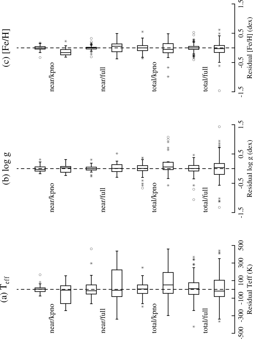
Figure 8: Boxplots illustrating comparisons between residuals obtained by the ANNs for the four data subsamples, in the sense $Q_{ANN}-Q_{CAT}$, where $Q$ represents the quantity $T_{\rm eff}$ (panel a), log ${\it g}$ (panel b), and [Fe/H] (panel c), respectively. The boxplots immediately above the subsample labels are those obtained from the training sets, while those immediately below the subsample labels are those obtained from the testing sets. The vertical line in each boxplot is the location of the median residual. The box extends to cover the central 50% of the data. The “whiskers” on each box extend to cover the last portion of the data not considered likely outliers. The asterisks and open circles indicate modest and large outliers, respectively.

Figure 8 is a graphical summary of the distribution of residuals for the three ANNs, grouped according to the training and testing data. In this figure, the training data is shown above the label for each subsample, and the testing data is shown below the label for each subsample. The vertical line in each boxplot is the location of the median residual. The box extends to cover the central 50% of the data (the inter-quartile range, $IQR$). The “whiskers” on each box extend to cover the last portion of the data not considered likely outliers (this range extends to cover the distance from the lower and upper ends of the $IQR$ + a factor of $1.5\;\times\;IQR$. The asterisks and open circles indicate modest and large outliers (lower and upper ends of the $IQR$ + a factor of $3.0\;\times\;IQR$), respectively. See Emerson & Strenio (1983) for a general discussion of boxplots.

The scales of the external errors in Table 4 provide our best estimates of the performance of the ANNs. The scale estimates obtained for the total/full subsample for each of the three ANNs, $S_{BI}(\mbox{$T_{\rm eff}$})=185$ K, $S_{BI}(\mbox{log ${\it g}$})=0.36$ dex, and $S_{BI}({\rm[Fe/H]})=0.21$ dex, are all acceptably low. Note that, in general, the scale estimates obtained for the nearby/kpno subsample are often somewhat smaller than those for the total/full subsample. We expect this result due to the more homogeneous nature and larger spectral coverage of the kpno data, relative to the full data. Furthermore, the spectra of the nearby stars typically have higher S/N than those included in the total/full subsample and, in the case of the log ${\it g}$ results, it should be kept in mind that the trigonometric gravities for the nearby stars are more accurate than those obtained for the more distant stars included in the total/full subsample.

Our external scale errors in the estimates of the atmospheric parameters include the errors in the determination of the parameters for the program stars, i.e., the catalog values. Given that the catalog values were drawn from a variety of sources, and no doubt incorporate a number of systematic offsets from star to star, we conservatively estimate that the errors of determination for the catalog values are of the order $\sigma(\mbox{$T_{\rm eff}$})\sim 100-125$ K, $\sigma(\mbox{log ${\it g}$})\sim 0.20-0.25$ dex, and $\sigma({\rm[Fe/H]})\sim 0.10-0.15$ dex, respectively. Subtracting these contributions to the external scale estimates obtained for the total/full subsample suggests that our likely errors in the physical quantities lie in the range $\sigma(\mbox{$T_{\rm eff}$})\sim 135-150$ K, $\sigma(\mbox{log ${\it g}$})\sim 0.25-0.30$ dex, and $\sigma({\rm[Fe/H]})\sim 0.15-0.20$ dex, respectively. The internal scale errors obtained from inspection of the training set for the total/full subsample are quite low, $S_{BI}(\mbox{$T_{\rm eff}$})=110$ K, $S_{BI}(\mbox{log ${\it g}$})=0.15$ dex, and $S_{BI}({\rm[Fe/H]})=0.09$ dex, suggesting that the intrinsic accuracy of our technique is limited by the accuracy of the training catalog values themselves, and not by any clear deficiency of the ANN approach.

Katz et al. (1998) have pursued a study of a least-squares matching technique, based on the comparison of high-resolution stellar spectra to a grid of stars with known atmospheric parameters, and obtained internal errors of estimation of $\sigma(\mbox{$T_{\rm eff}$})\sim 85-100$ K, $\sigma(\mbox{log ${\it g}$})\sim 0.28$ dex, and $\sigma({\rm[Fe/H]})\sim 0.17$ dex, respectively, for stellar spectra with S/N ratios in the range 10 to 100. These errors are completely in line with our own internal errors, suggesting that, when applying the ANN technique, one is not forced to employ high-resolution spectroscopy, at least for accurate determination of these stellar parameters.

5.3 Limitations of the ANN Approach, and Deviations from the General Trends

The scatter of points seen in Figure 8 is dominated by a small number of stars with large mismatches between input catalog parameters and output network predictions. Blame for these clashes must be assessed on a case-by-case basis, and is provided in Appendix A. Included in that list are stars with $\mid$ANN-CAT$\mid$ parameter deviations in excess of 350 K in $T_{\rm eff}$, 0.6 dex in log ${\it g}$, and 0.3 dex in [Fe/H]. Below we discuss some factors that may be responsible when good points go bad.

The reader is cautioned again that the ANNs of this study, in common with all automated pattern recognition algorithms, are far better interpolators than extrapolators. Our ANNs have trouble in those areas of the ($T_{\rm eff}$, log ${\it g}$, [Fe/H]) parameter space where the training spectra are few or absent. For example, from inspection of the middle panel of Figure 4 one expects difficulties for stars with [Fe/H] $\lesssim$ –3, especially over the temperature regime 5000 $<$ $T_{\rm eff}$ $<$ 6000 K, where we have no training or test spectra. Five of the deviant stars discussed in Appendix A have extremely low metallicities, and their spectra at moderate resolution have very few strong atomic features. The ANNs undoubtedly are losing some parameter sensitivity in this metallicity regime, a limitation that should be easily overcome by training on larger samples of lower metallicity stars.

Subgiants, those stars in the parameter space defined roughly by 5100 $<$ $T_{\rm eff}$ $<$ 5600 K and 3.2 $<$ log ${\it g}$ $<$ 3.8 (Figure 4, top panel), are apparently not well represented among our program stars. However, this gap may be, at least in part, tied to our adopted methods of setting catalog parameters for the program stars. One virtue of the approach outlined in §4 lies in its uniformity – every star is treated as identically as possible. But this demands that some more-or-less arbitrary choices be made. For example, the adopted temperature scale is that of Alonso et al. (1996, 1999), which is based upon application of the IRFM. The IRFM has very few input assumptions, but does rely on model atmospheres to predict monochromatic IR fluxes. On the other hand, the adopted gravities are derived from the absolute magnitudes of Beers et al. (1999), based on a visual spectral classification. Consider as one example the well-studied subgiant HD 140283. Our application of the Alonso temperature calibration yields $T_{\rm eff}$ _CAT = 5792 K, but a glimpse at several recent high-resolution analyses shows a wide range of values: 5640 K (Magain 1989 $\equiv$ M89), 5750 K (Ryan, Norris, & Beers 1996 $\equiv$ RNB96), 5755-5779 (Gratton, Carretta, & Castelli 1996 $\equiv$ GCC96), and 5843 K (Fuhrmann et al. 1997 $\equiv$ FPFRG97). This particular case exemplifies a general tendency: the temperature scales from the IRFM advocated by Alonso et al. are neither among the highest nor the lowest scales in the literature. We assigned log ${\it g}$ ${}_{\rm CAT}=3.75$ to this star, close to the highest values among the high-dispersion studies: 3.10 (M89), 3.40 (RNB6), 3.60-3.80 (GCC96), and 3.20 (FPFRG97). However, Allende Prieto et al. (1999) derived $\log g\sim$ 3.80 from the measured Hipparcos parallax. Finally, [Fe/H]${}_{\rm CAT}=-2.47$, which falls in the middle of the range spanned by the high-dispersion analyses: $-2.70$ (M89), $-2.54$ (RNR96), $-2.38$ to $-2.42$ (GCC96), and $-2.34$ (FPFRG97).

We want to emphasize that considerable care is required in the examination of the temperature, gravity, and metallicity scales adopted in this and in other studies. The same warning applies to individual cases of deviations between input catalog and output ANN parameters, as not all of our program stars have been treated with equal vigor in past studies. Indeed, a few of our program stars have not yet had the benefit of high-resolution spectroscopic analysis over wide wavelength ranges. The ANNs constructed here may fail for particular stars, but often they also bring to light stars that deserve further study.

5.4 Experiments on Spectra with Artificially Increased Noise

If ANNs are to be successfully employed in the analysis of extremely large spectroscopic data sets (which we anticipate will become available in the near future), they will need to work reliably on spectra with both high S/N, like the spectra employed here, as well as with spectra of much lower S/N. Our data are not ideally suited to explore the effects of variable S/N values on ANNs, but we have attempted a few experiments that may point the way toward more comprehensive efforts in the future.

From our original sample of program stars we randomly selected a subset of 52 stars having S/N $\sim$ 50 near 4000 Å, and artificially degraded their S/N at this wavelength to $\sim$ 26 and then to $\sim$ 13. The strong wavelength dependence of the S/N in the original spectra was preserved using the square root of the raw (unflattened) spectra to scale the extra poissonian noise introduced. In Figure 9 we display one example of the S/N degradation procedure. The pernicious effect of low S/N is clearly seen in this figure, as some prominent features (e.g., the CH G-band near 4300 Å, or Fe I at 4045 Å) in the original spectrum shown in the top panel become nearly undetectable in the low S/N spectrum shown in the bottom panel.

As a first experiment, we submitted these sets of spectra with different noise levels as new data into the final ANNs that we had trained as described above. In this manner, we sought to ascertain whether or not the ANNs built to recognize differences in high S/N spectra could produce reasonable estimates of the atmospheric parameters for stars with lower S/N spectra.

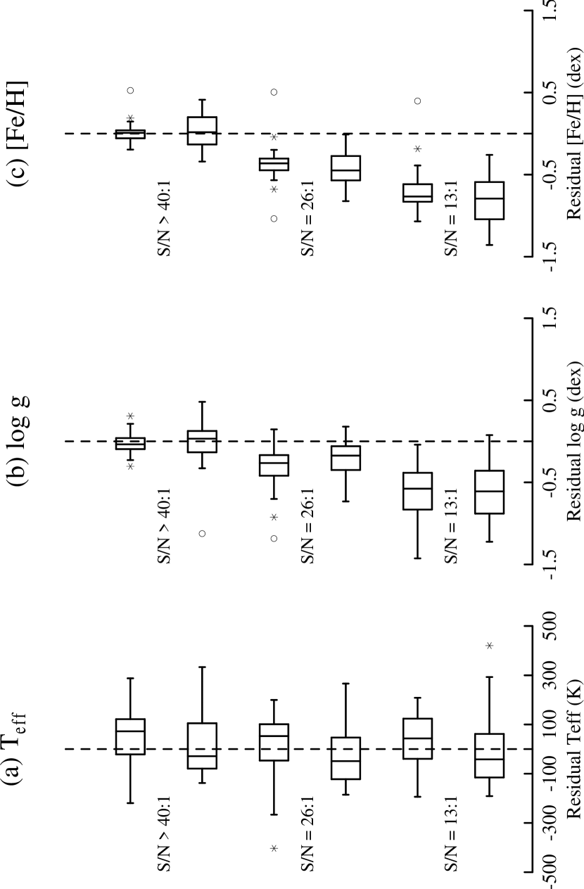
Figure 10: Boxplots illustrating comparisons between residuals obtained by the ANNs for the S/N exploration subsamples, in the sense $Q_{S/N}-Q_{S/N>40}$, where $Q$ represents the quantity $T_{\rm eff}$ (panel a), log ${\it g}$ (panel b), and [Fe/H] (panel c), respectively. The boxplots immediately above the subsample labels are those obtained from the training sets, while those immediately below the subsample labels are those obtained from the testing sets. Note the obvious systematic offsets in estimated log ${\it g}$ and [Fe/H] for the lower S/N subsamples.

In Table 5 we summarize the statistics of the ANN classifications of these data sets, organized in a similar manner to Table 4 above. Figure 10 is a graphical summary of the distribution of residuals for this experiment. Inspection of the table and figure reveal several features of note. As expected, there is a clear general trend toward increasing the zero point error ($C_{BI}$) and in the scatter ($S_{BI}$) for both the internal and external subsamples as one progresses to lower S/N ratios. The $T_{\rm eff}$ classification is the least affected, with the changes in location and scale of the residuals staying almost constant as one progresses from high to low S/N ratios. The log ${\it g}$ classification suffers rapid degradation with declining S/N, and exhibits a systematic shift in the zero point from near $0.0$ dex to on the order of $-0.6$ to $-0.7$ dex, and roughly a tripling of the scatter. Similarly, the [Fe/H] classification indicates a zero-point shift and increase in scatter with declining S/N.

The systematic errors in [Fe/H] are puzzling, and opposite those seen in the auto-correlation function approach described by Beers et al. (1999), where decreasing S/N leads to a positive systematic error in the metallicity scale. Furthermore, there also exists a trend in metallicity at a fixed S/N ratio, in the sense that metal-rich stars have their abundances more underestimated than the metal-deficient stars. At present, we cannot explain these systematic trends in log ${\it g}$ or [Fe/H] classification with decreasing S/N, and we leave this to future investigation.

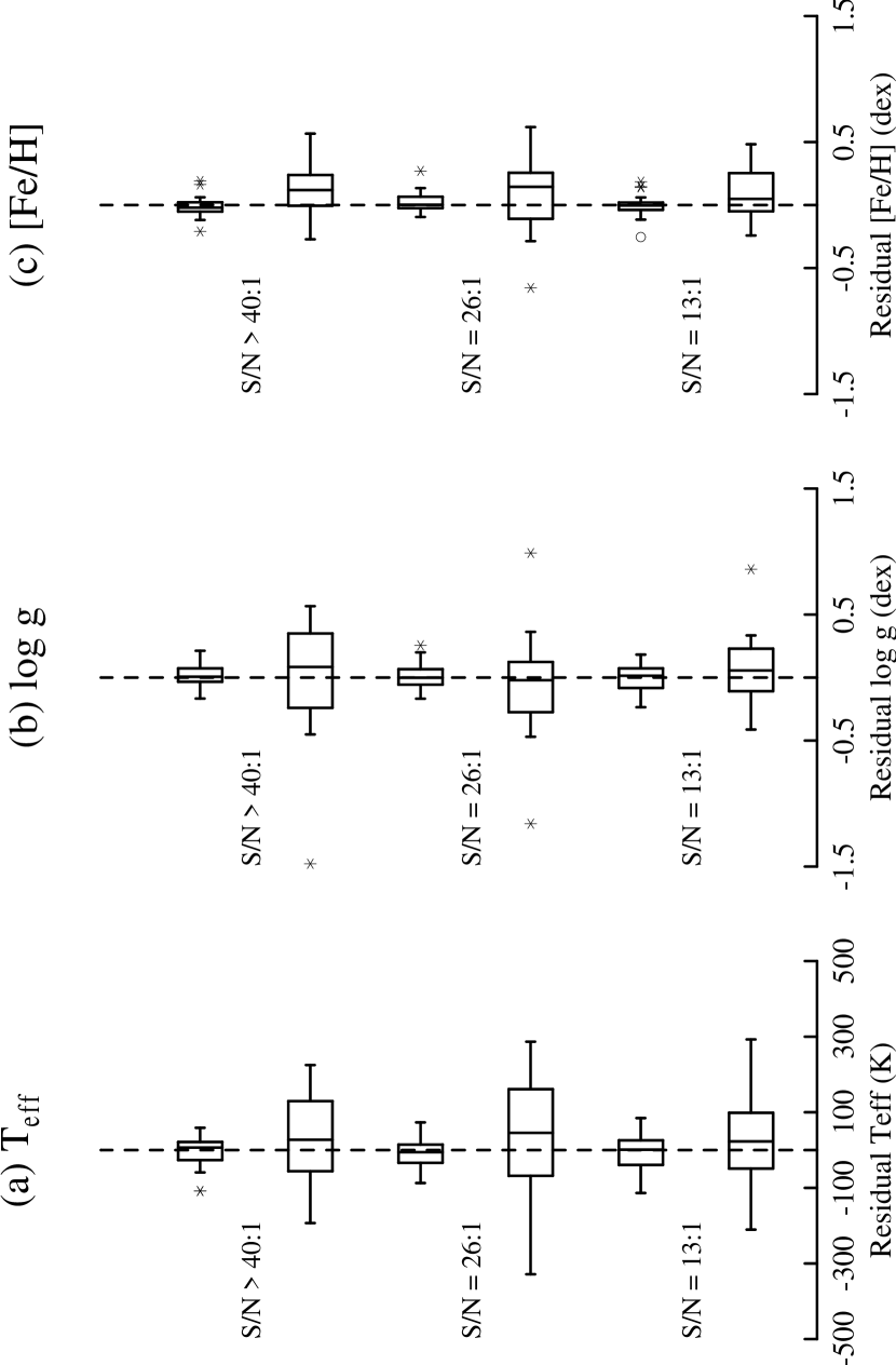
Figure 11: Boxplots illustrating comparisons between residuals obtained by the ANNs for the S/N exploration subsamples, for $T_{\rm eff}$(panel a), log ${\it g}$(panel b), and [Fe/H] (panel c), respectively. The boxplots immediately above the subsample labels are those obtained from the training sets, while those immediately below the subsample labels are those obtained from the testing sets. Note that in this case, where the ANNs are trained on spectra of similar S/N ratios as that of the spectra which are submitted to them for evaluation, the systematic offsets seen in Figure 10 disappear.

As a final experiment, we constructed new ANNs, trained on input spectra having similar S/N ratios to the spectra we test them with, i.e.  S/N $>40$, $26$, and $13$ respectively. Table 5 and Figure 11 show the results. It is immediately clear that the zero-point shifts previously encountered have now disappeared. Of even greater interest, the scatter obtained in the estimates of the internal and external errors are essentially identical for spectra of declining S/N ratios, and are roughly equivalent to those obtained previously when using ANNs trained and tested with only high S/N spectra, as can be noted by comparison of Figure 10 with Figure 8. We conclude that it is better to classify spectra of a given S/N with ANNs trained on spectra of similar S/N than with ANNs trained exclusively on higher S/N spectra. This result suggests two future approaches. One should either train ANNs on spectra with a variety of S/N ratios (and much larger training sets), or train ANNs for specific S/N ratios, and carry out an interpolation between the derived results for the observed S/N of the spectrum.

6 Conclusions

We have explored the use of artificial neural networks for three-dimensional classification of medium-resolution stellar spectra. We have constructed, trained, and tested ANNs specific to the individual estimation of the $T_{\rm eff}$, log ${\it g}$, and [Fe/H], and find that these parameter-specific networks are superior to the simultaneous estimation of multiple parameters from an omnibus ANN. The external accuracy of the physical parameter estimates, $\sigma(\mbox{$T_{\rm eff}$})=135-150$ K over the range $4250\leq\mbox{$T_{\rm eff}$}\leq 6500$ K, $\sigma(\mbox{log ${\it g}$})=0.25-0.30$ dex over the range $1.0\leq\mbox{log ${\it g}$}\leq 5.0$ dex, and $\sigma({\rm[Fe/H]})=0.15-0.20$ dex over the range $\-4.0\leq{\rm[Fe/H]}\leq+0.3$, strongly encourage further refinement of this approach for future work. Furthermore, we find that the derived accuracies of parameter estimates are not severely affected by the presence of modest spectral noise, at least when networks are trained with spectra with similar S/N ratios to those that will be analyzed. Further experimentation is necessary to identify the limiting S/N ratio for which useful parameter estimation is still possible; already, we find reasonably accurate estimates can be obtained with spectra of S/N as low as 13.

In the near future, we anticipate the construction of trained ANNs, covering a variety of S/N ratios and spectral resolutions, with which stellar spectra exhibiting a wide range of atmospheric parameters can be usefully analyzed. The recent study by Gray, Graham & Hoyt (2001), which makes use of stellar spectra very similar to those employed here, has revealed that micro-turbulence has to be taken into account as an independent parameter in order to recover properly the surface gravity. A second addition that will improve the results is to decouple the abundances of the alpha elements from the rest of the metals, modeling it as a new variable. So far, the simple tests carried out in this paper encourage the use and refinement of ANNs for on-going and soon-to-be-undertaken large-scale surveys of stellar spectra, both from ground-based and space-based observatories.

Appendix A Comments on Deviant Stars

In spite of the excellent general predictive capability of our ANNs, some stars obviously have poor matches between one or more of their CAT and ANN atmospheric parameters. In this appendix we draw attention to those cases with parameter clashes $\mid$CAT–ANN$\mid$ that are larger than 350 K in $T_{\rm eff}$, 0.6 dex in log ${\it g}$, and 0.3 dex in [Fe/H]. The discrepant cases are noted in Table 2 and Table 3 with a colon next to the relevant parameters. Since one expects (and we found) a larger overall agreement for the training set than for the testing set, these subsets will be considered separately. We refer the reader back to Figures 5–7 to visually locate these deviant stars in relation to the vast majority of conforming stars.

For each star only the deviating parameters will be quoted here; see Tables 2 and 3 for the remaining parameters. Comments given here will primarily address comparisons with previous papers that report extensive abundance analyses from high-resolution spectroscopy. Several useful papers discuss the derivation of atmospheric parameters for large stellar samples from medium-resolution ($R\equiv\lambda$/$\Delta\lambda\sim$ 5000) spectra (e.g., Beers et al. 1999; Ryan & Norris 1991), or from very low S/N, small wavelength-coverage spectra (e.g., Carney et al. 1994, and references therein). Such studies have formed the basis for compilation of our catalog parameters, so will not be re-examined in detail here. In citing literature sources to support catalog or ANN parameters, it should be understood that although the results of various studies are hopefully internally self-consistent, in our application they were normalized to a variety of $T_{\rm eff}$, log ${\it g}$, and [Fe/H] systems. Consequently, the reader is urged to view the following comments with indulgence.

First we consider the parameter mismatches in the ANN training set. Two stars of this set have not been studied extensively with high-spectral resolution data: G 66-49 ([Fe/H]_CAT = –0.57, [Fe/H]_ANN = –0.13), and G 236-11 ([Fe/H]_CAT = +0.31, [Fe/H]_ANN = –0.10). Note that the Beers et al. (1999) medium-resolution study obtained estimates of metallicity of [Fe/H]${}_{\rm AK2}=-0.32$ for G 66-49 and [Fe/H]${}_{\rm AK2}=-0.20$ for G 236-11, closer to the predictions of the ANN. These two stars will not be discussed further here. For the handful of other discrepant stars, we list below a few brief comparisons to the literature.

• BD $+$37 1458 (log ${\it g}$ _CAT = 4.71, log ${\it g}$ _ANN = 4.00): This star’s Hipparcos parallax (ESA 1997) is consistent with subgiant evolutionary status, and Gratton et al. (2000) derive log ${\it g}$ = 3.3, thus the ANN gravity value is clearly to be preferred over that of the catalog.

• CS 22949-037 ([Fe/H]_CAT = –3.99, [Fe/H]_ANN = –3.46): This extremely metal-poor star is warm enough to have little heavy-element line absorption at moderate spectral resolution. The ANN can recognize the star’s low metallicity, but cannot be expected to derive a very accurate abundance estimate due to the few training stars at such low metallicities and intermediate temperatures. Nevertheless, comparison with the recent high-resolution analysis of Norris, Ryan, & Beers (2001), who obtain [Fe/H] = –3.79, indicates that the correct abundance lies roughly halfway between the CAT and ANN values. Note that the Beers et al. (1999) abundance, [Fe/H]${}_{\rm AK2}=-3.46$, exactly matches the ANN determination.

• G 58-30 = HD 94835 ([Fe/H]_CAT = +0.30, [Fe/H]_ANN = –0.05): Feltzing & Gustafsson (1998) derive [Fe/H] = +0.13, splitting the difference between the catalog and ANN values. The Beers et al. (1999) abundance estimate for this star is [Fe/H]${}_{\rm AK2}=-0.32$, closer to the ANN value.

• HD 84937 ([Fe/H]_CAT = –2.06, [Fe/H]_ANN = –2.37): Carretta, Gratton, & Sneden (2000) derive [Fe/H] = –2.04 from a reanalysis of literature data; the approximate mean value of other recent literature sources (Cayrel de Strobel et al. 1997) suggests [Fe/H] = –2.2, so the catalog metallicity is probably to be preferred. The Beers et al. (1999) estimate for HD 84937 is [Fe/H]${}_{\rm AK2}=-2.14$, closer to the catalog abundance estimate.

• HD 105546 ($T_{\rm eff}$ _CAT = 4727 K, $T_{\rm eff}$ _ANN = 5095 K): The ANN temperature is in better agreement with high-resolution spectroscopic studies: $T_{\rm eff}$ = 5300 K (Pilachowski, Sneden, & Kraft 1996), and $T_{\rm eff}$ = 5147 K (Gratton et al. 2000).

• HD 136202 (log ${\it g}$ _CAT = 5.70, log ${\it g}$ _ANN = 4.64): The latest update of the Cayrel de Strobel et al. (1997) catalog lists literature studies deriving $<$log ${\it g}$$>$ = 4.0. The SIMBAD database lists a spectral type of F8 III-IV. Therefore the inferred extremely high catalog log ${\it g}$ is incorrect.

• HD 218857 ($T_{\rm eff}$ _CAT = 5165 K, $T_{\rm eff}$ _ANN = 4740 K): Previous high-resolution analyses (e.g., $T_{\rm eff}$ = 5125 K, Pilachowski et al. 1996) and $B-V$ = 0.65 from the SIMBAD database support the higher catalog temperature.

• LP 685-44 ($T_{\rm eff}$ _CAT = 5290 K, $T_{\rm eff}$ _ANN = 4726 K): No extensive analysis of this star using high spectral resolution data has been published. The SIMBAD database has $B-V$ = 0.63, consistent with the higher catalog $T_{\rm eff}$.

Next we consider parameter estimation problems in the testing set of stars. The discrepant stars of this set that apparently lack extensive high-resolution spectroscopic analyses are:

G 17-22 = HD 149162 ($T_{\rm eff}$ _CAT = 4765 K, $T_{\rm eff}$ _ANN = 5687 K); G 99-52 ([Fe/H]_CAT = –1.40, [Fe/H]_ANN = –2.01); G 106-53 ([Fe/H]_CAT = –0.21, [Fe/H]_ANN = –0.58); G 146-76 (log ${\it g}$ _CAT = 4.69, log ${\it g}$ _ANN = 3.57); and G 161-84 ($T_{\rm eff}$ _CAT = 4605 K, $T_{\rm eff}$ _ANN = 5013 K). The Beers et al. (1999) abundance determination for G 99-52 is [Fe/H]${}_{\rm AK2}=-0.87$, while that for G 106-53 is [Fe/H]${}_{\rm AK2}=-0.31$. These stars will not be discussed further here. Below we list comments based on comparisons with the literature for this somewhat larger list of discrepant stars.

• BD $+$01 2916 ($T_{\rm eff}$ _CAT = 4247 K, $T_{\rm eff}$ _ANN = 4782 K; log ${\it g}$ _CAT = 1.02, log ${\it g}$ _ANN = 1.83; [Fe/H]_CAT = –1.82, [Fe/H]_ANN = –2.37): High-resolution studies (Cayrel de Strobel et al. 1997, Shetrone 1996) favor the catalog values of all parameters. The Beers et al. (1999) abundance determination for this star, [Fe/H]${}_{\rm AK2}=-1.60$, seems to support the catalog value as well.

• BD $-$04 680 ($T_{\rm eff}$ _CAT = 5650 K, $T_{\rm eff}$ _ANN = 5902 K; [Fe/H]_CAT = –2.22, [Fe/H]_ANN = –1.81): Bonifacio & Molaro (1997) recommend $T_{\rm eff}$ = 5866 K, log ${\it g}$ =3.73, and [Fe/H] = –2.07, in rough agreement with the means of the CAT and ANN temperatures and metallicities, but their gravity value is much lower than either of our estimates, so further investigation of this star is warranted. The Beers et al. (1999) abundance determination for this star, [Fe/H]${}_{\rm AK2}=-2.17$, agrees well with the catalog estimate.

• BD $-$14 5890 (log ${\it g}$ _CAT = 2.27, log ${\it g}$ _ANN = 3.01): The analysis of Bonifacio, Centurion, & Molaro (1999), drawing on results of an earlier study by Cavallo, Pilachowski, & Rebolo (1997), yields gravity estimates of log ${\it g}$ = 2.34 from the star’s Hipparcos parallax, and log ${\it g}$  = 1.4 from a spectrum analysis; these appear to rule out the higher ANN gravity. Note also that Bonifacio et al. derived [Fe/H] = –2.52, substantially lower than either of our metallicity estimates. The Beers et al. (1999) abundance determination for this star is [Fe/H]${}_{\rm AK2}=-2.07$, midway between the CAT and ANN values, and again, rather different from the Bonifacio et al. estimate.

• CS 22873-128 (log ${\it g}$ _CAT = 2.50, log ${\it g}$ _ANN = 3.37): McWilliam et al. (1995) derive log ${\it g}$  = 2.1 for this extremely metal-poor giant, and our ANN probably does not have many good log ${\it g}$ indicators in this cool star’s very weak-lined spectrum.

• CS 22891-200 ($T_{\rm eff}$ _CAT = 4632 K, $T_{\rm eff}$ _ANN = 5053 K; log ${\it g}$ _CAT = 1.87, log ${\it g}$ _ANN = 4.02; [Fe/H]_CAT = –3.49, [Fe/H]_ANN = –2.88): The McWilliam et al. (1995) high-dispersion analysis provides a temperature estimate, $\mbox{$T_{\rm eff}$}=4700$ K, that matches the catalog value, but differs somewhat in its derived surface gravity estimate, $\mbox{log ${\it g}$}=1.0$. The ANN log ${\it g}$ is clearly incorrect.

• CS 22968-014 ($T_{\rm eff}$ _CAT = 4815 K, $T_{\rm eff}$ _ANN = 5335 K; log ${\it g}$ _CAT = 2.24, log ${\it g}$ _ANN = 2.96; [Fe/H]_CAT = –3.43, [Fe/H]_ANN = –2.94): The McWilliam et al. (1995) high-dispersion analysis completely supports the catalog values for this star – yet another example of our trained ANNs having trouble with a cool, very weak-lined spectrum. The Beers et al. (1999) abundance determination for this star, [Fe/H]${}_{\rm AK2}=-3.35$, is closer to the catalog value.

• G 21-22 ($T_{\rm eff}$ _CAT = 6167 K, $T_{\rm eff}$ _ANN = 5828 K; log ${\it g}$ _CAT = 3.70, log ${\it g}$ _ANN = 4.64; [Fe/H]_CAT = –0.88, [Fe/H]_ANN = –1.18): Bonifacio & Molaro (1997) derive $T_{\rm eff}$ = 5869 K, log ${\it g}$ = 3.93, and [Fe/H] = –1.63, thus agreeing with the ANN result for temperature, with the catalog input for gravity, and with neither for metallicity! The Beers et al. (1999) abundance determination for G 99-52 is [Fe/H]${}_{\rm AK2}=-0.87$, in agreement with the catalog estimate. This obviously is a case for further exploration on all fronts.

• HD 6755 ($T_{\rm eff}$ _CAT = 5230 K, $T_{\rm eff}$ _ANN = 4864 K; [Fe/H]_CAT = –1.49, [Fe/H]_ANN = –1.98): All of the literature (Cayrel de Strobel et al. 1997) studies support the catalog values for this star, as does the Beers et al. (1999) abundance determination, [Fe/H]${}_{\rm AK2}=-1.35$; the ANN result is clearly in error.

• HD 20038 (log ${\it g}$ _CAT = 2.41, log ${\it g}$ _ANN = 3.21): Gratton et al. (2000) derive log ${\it g}$ = 2.38, so the catalog value is to be preferred.

• HD 44007 (log ${\it g}$ _CAT = 2.71, log ${\it g}$ _ANN = 1.61): The mean of the entries in Cayrel de Strobel et al. (1997) suggest log ${\it g}$ $\simeq$ 2.1, nearly splitting the difference between the CAT and ANN values.

• HD 74462 (log ${\it g}$ _CAT = 2.91, log ${\it g}$ _ANN = 1.89): Most previous studies (Cayrel de Strobel et al. 1997) support the ANN value, and Gratton et al. (2000) derive log ${\it g}$ =1.56, thus the catalog entry appears incorrect.

• HD 111721 (log ${\it g}$ _CAT = 3.01, log ${\it g}$ _ANN = 1.46; [Fe/H]_CAT = –1.26, [Fe/H]_ANN = –2.72): The high-resolution analysis of Gratton et al. (2000) obtains log ${\it g}$ = 2.5 and [Fe/H] =–1.27, in support of the catalog values. The Beers et al. (1999) abundance determination for this star is [Fe/H]${}_{\rm AK2}=-0.88$, also in better agreement with the catalog value.

• HD 128279 (log ${\it g}$ _CAT = 3.11, log ${\it g}$ _ANN = 4.54): This star is clearly evolved from the main sequence, as Pilachowski et al. (1996) derive log ${\it g}$ =2.8, and Gratton et al. (2000) obtain a value of 3.0. The catalog gravity is correct.

• HD 187111 ($T_{\rm eff}$ _CAT = 4247 K, $T_{\rm eff}$ _ANN = 4688 K): Most literature sources (Cayrel de Strobel et al. 1997) agree with the lower catalog temperature, but Gratton et al. (2000) derive $T_{\rm eff}$ =4429, in the middle of the CAT / ANN range.

• HD 195636: Although the CAT and ANN parameters do not disagree enough to qualify as discrepant here, we note that this unique star has been described by Preston (1997) as a star near the transition region between the horizontal and asymptotic giant branches. It also is rapidly rotating for a highly evolved star: v$sini$ = 25 km s^-1. Its line spectrum will not fit easily into classification schemes based on more normal metal-poor stellar spectra.

• HD 196944 (log ${\it g}$ _CAT = 2.89, log ${\it g}$ _ANN = 1.57; [Fe/H]_CAT = –2.33, [Fe/H]_ANN = –1.95): This is a carbon-rich metal-poor star, and our ANNs have not been properly trained to deal with spectra of those objects. But the detailed analysis of Zacs, Nissen, & Schuster (1998) yields log ${\it g}$ =1.7 and [Fe/H] = –2.45, strongly supporting the ANN gravity while in closer agreement with the catalog [Fe/H] value.

• LP 815-43 ([Fe/H]_CAT = –3.20, [Fe/H]_ANN = –2.79) Ryan, Norris & Bessel (1991) obtain [Fe/H] = –3.20, and all agree that the star is a warm main-sequence star; its very weak-lined spectrum is clearly difficult for our ANN to treat properly for metallicity. However, the Beers et al. (1999) abundance determination for this star is [Fe/H]${}_{\rm AK2}=-2.92$, closer to the ANN value.

• Ross-740 = LTT 743 ($T_{\rm eff}$ _CAT = 5010 K, $T_{\rm eff}$ _ANN = 5968 K): Ryan, et al. (1991) derive $T_{\rm eff}$ =5500, log ${\it g}$ =3.2, [Fe/H] = –2.75, and Beers et al. (1999) obtain [Fe/H]${}_{\rm AK2}=-2.91$, so both of our metallicity estimates appear to be reasonable, but both the catalog and the ANN claim main-sequence gravity for a star that seems to be a subgiant from high-resolution analysis.

Table 1: The Spectroscopic Data Sets

Telescope	Detector	Coverage	Dispersion	Number
		(Å)	(Å/pix)
ESO 1.5m	Ford + Loral 2048$\times$2048	3750$-$4750	0.65 + 0.50	52
KPNO 2.1m	Tek 2048$\times$2048	3750$-$5000	0.65	115
LCO 2.5m	Reticon + 2D-Frutti	3700$-$4500	0.65	50
ORM INT 2.5m	Tek 1024$\times$1024	3750$-$4700	0.85	3
PAL 5m	Reticon + 2D-Frutti	3700$-$4500	0.65	3
SSO 2.3m	SITe 1752$\times$532	3750$-$4600	0.50	58

Note. — ESO $\equiv$ European Southern Observatory; KPNO $\equiv$ Kitt Peak National Observatory; LCO $\equiv$ Las Campanas Observatory; ORM $\equiv$ Observatorio del Roque de los Muchachos; PAL $\equiv$ Palomar Observatory; SSO $\equiv$ Siding Spring Observatory

Table 2: Catalog and ANN Parameters for the Training Sample

Star	Source	T${}_{\rm eff~{}CAT}$	T${}_{\rm eff~{}ANN}$	$\log g_{\rm CAT}$	$\log g_{\rm ANN}$	[Fe/H]CAT	[Fe/H]ANN
		(K)	(K)	(dex)	(dex)	(dex)	(dex)
BD +03 2782	K	4790	4770	2.32	2.29	$-$2.02	$-$2.05
BD +04 2621	K	4712	4795	1.71	1.83	$-$2.41	$-$2.43
BD +06 648	K	4455	4633	0.97	0.91	$-$2.09	$-$2.11
BD +09 2870	K	4672	4749	1.62	1.53	$-$2.39	$-$2.31
BD +09 352	E	6050	5987	4.14	4.25	$-$2.09	$-$2.09
BD +10 2495	K	4875	4884	2.81	3.05	$-$1.83	$-$2.12
BD +17 3248	K	4995	5042	2.94	2.73	$-$2.03	$-$2.13
BD +17 4708	O	6085	6092	4.50	4.25	$-$1.72	$-$1.79
BD +19 1185	K *	5435	5427	4.38	4.31	$-$1.33	$-$1.22
BD +30 2611	K	4362	4642	1.12	1.27	$-$1.32	$-$1.38
BD +37 1458	K	5422	5181	4.71:	4.00:	$-$1.95	$-$2.09
BD $-$01 2582	E	5145	5125	4.61	4.71	$-$2.23	$-$2.16
BD $-$13 3442	E	6160	6276	4.29	4.28	$-$3.14	$-$3.08
BD $-$18 5550	K	4785	4963	1.87	1.88	$-$2.89	$-$2.83
CD $-$31 622	L	5285	5224	4.75	4.68	$-$2.00	$-$2.04
CD $-$33 3337	L	5930	6069	4.11	4.09	$-$1.40	$-$1.32
CD $-$71 1234	E	6082	6297	4.29	4.40	$-$2.65	$-$2.57
CS 22873-055	L	4675	4700	1.53	1.54	$-$2.88	$-$2.94
CS 22873-166	L	4605	4600	1.30	1.16	$-$2.90	$-$2.95
CS 22878-101	E	4757	4947	2.14	1.94	$-$3.13	$-$3.10
CS 22892-052	E	4640	4632	1.91	1.96	$-$3.01	$-$2.99
CS 22896-154	L	5107	5032	2.94	2.84	$-$2.73	$-$2.72
CS 22947-187	E	5077	5251	2.80	2.69	$-$2.49	$-$2.50
CS 22949-037	P	4810:	5097:	2.16	2.05	$-$3.99:	$-$3.46:
CS 22952-015	P	4667	4666	1.95	1.85	$-$3.26	$-$3.32
G 5-19	K	5607	5606	4.45	4.54	$-$1.55	$-$1.50
G 8-16	K *	6020	6089	4.12	4.07	$-$1.59	$-$1.68
G 9-27	K	5440	5383	4.57	4.55	$-$1.78	$-$1.82
G 10-26	S *	5900	5915	4.25	4.35	$-$0.03	$-$0.13
G 11-36	S *	5682	5583	4.32	4.40	$-$0.68	$-$0.56
G 11-37	K *	5287	5228	4.85	4.77	$-$0.14	$-$0.19
G 11-44	K	6010	6082	4.18	4.18	$-$2.07	$-$2.05
G 11-45	K *	5490	5535	4.82	4.93	$-$0.01	$-$0.03
G 13-1	S *	5817	5792	4.67	4.58	$-$0.25	$-$0.22
G 13-9	K	6082	6270	4.24	4.22	$-$2.31	$-$2.26
G 13-38	S *	5220	5204	4.60	4.66	$-$0.96	$-$0.96
G 14-5	S *	5342	5507	4.65	4.63	$-$0.70	$-$0.57
G 14-24	K	4970	4815	4.76	4.85	$-$2.17	$-$2.22
G 14-26	S	5800	5772	4.40	4.66	$-$0.20	$-$0.20
G 14-38	S	5235	5180	4.75	4.76	$-$0.42	$-$0.24
G 14-54	S	5612	5490	4.57	4.73	$-$0.13	$-$0.14
G 16-9	E *	4892	4903	4.89	4.89	$-$0.77	$-$0.72
G 16-13	S	5562	5460	4.40	4.40	$-$1.03	$-$1.01
G 16-31	S *	4890	4753	4.82	4.84	$-$0.55	$-$0.63
G 17-16	E	5190	5216	4.61	4.50	$-$0.83	$-$0.76
G 17-21	L *	5835	5873	4.27	4.44	$-$0.66	$-$0.64
G 17-29	E *	5322	5311	4.95	5.23	$+$0.05	$+$0.02
G 17-30	S *	5600	5672	4.57	4.69	$-$0.48	$-$0.42
G 18-40	K	5800	5778	4.24	4.46	$-$1.76	$-$1.75
G 20-8	E	5957	6066	4.23	4.19	$-$2.30	$-$2.27
G 22-20	E	6060	5898	3.86	4.32	$-$0.82	$-$1.07
G 23-14	K	4922	5000	4.87	4.60	$-$2.05	$-$1.92
G 23-16	K *	4900	4773	4.97	5.01	$-$0.03	$-$0.02
G 24-15	L *	5912	5926	4.09	4.06	$-$1.10	$-$1.12
G 24-17	K *	4777	4639	4.78	4.60	$-$0.95	$-$0.94
G 24-18F	K *	4767	4602	4.91	4.74	$-$0.87	$-$0.84
G 28-31	L	5762	6009	4.39	4.34	$-$2.22	$-$2.16
G 29-25	K	5340	5372	4.46	4.54	$-$0.99	$-$0.86
G 29-71	K	5685	5585	4.48	4.26	$-$2.26	$-$2.34
G 31-26	K	5345	5389	4.51	4.84	$-$1.49	$-$1.51
G 37-26	L *	5940	5860	4.21	4.08	$-$1.93	$-$1.87
G 40-14	S	6257	6260	4.20	3.98	$-$2.54	$-$2.55
G 43-5	K	5310	5210	4.66	4.58	$-$2.12	$-$2.09
G 43-30	K *	5120	5108	5.05	4.92	$-$0.12	$+$0.02
G 43-33	L *	5925	5899	4.30	4.42	$-$0.37	$-$0.26
G 43-44	K *	5307	5114	4.90	5.07	$-$0.08	$-$0.06
G 44-6	S *	5617	5629	4.61	4.60	$-$0.54	$-$0.63
G 44-30	S	5425	5405	4.49	4.62	$-$0.89	$-$0.88
G 46-31	S	5772	5706	4.29	4.42	$-$0.89	$-$0.90
G 48-29	L	6257	6373	4.22	4.16	$-$2.50	$-$2.53
G 53-30	S	5450	5492	4.57	4.65	$-$0.43	$-$0.39
G 53-41	L	5967	5951	3.91	3.73	$-$1.21	$-$1.20
G 54-21	K *	5862	5788	4.48	4.64	$-$0.03	$-$0.17
G 56-48	K	4775	4673	4.78	4.85	$-$2.20	$-$2.20
G 58-23	K *	5540	5456	4.40	4.43	$-$0.97	$-$0.90
G 58-25	K *	5930	5908	4.01	4.07	$-$1.41	$-$1.37
G 58-30	K *	5855	5803	4.70	4.62	$+$0.30:	$-$0.05:
G 58-41	K *	5865	5869	4.39	4.33	$-$0.33	$-$0.46
G 59-1	K	5430	5353	4.56	4.43	$-$1.02	$-$0.74
G 59-27	K	6092	6136	4.09	4.16	$-$2.10	$-$2.08
G 60-46	S	5300	5160	4.59	4.59	$-$1.19	$-$1.28
G 60-48	L	5817	5835	4.28	4.15	$-$1.63	$-$1.62
G 62-44	S *	5102	5024	4.87	4.81	$-$0.58	$-$0.29
G 62-52	K *	5252	5224	4.59	4.62	$-$1.28	$-$1.36
G 62-61	S *	5830	5733	4.52	4.39	$-$0.32	$-$0.31
G 64-12	K	6272	6354	4.28	4.13	$-$3.31	$-$3.16
G 64-37	E	6377	6367	4.20	4.01	$-$3.00	$-$3.04
G 64-54	S *	5332	5361	4.89	4.91	$-$0.10	$-$0.28
G 65-47	S *	5607	5598	4.58	4.72	$-$0.35	$-$0.36
G 66-9	E	5685	5747	4.49	4.51	$-$2.23	$-$2.24
G 66-15	S *	5590	5375	4.53	4.61	$-$0.20	$-$0.46
G 66-49	S *	5345	5478	4.74	4.86	$-$0.57:	$-$0.13:
G 75-56	K	6040	6238	4.19	4.13	$-$2.33	$-$2.21
G 79-42	K	5635	5655	4.32	4.36	$-$1.10	$-$1.16
G 80-15	K *	5800	5823	4.23	4.35	$-$0.78	$-$0.81
G 82-42	K	5535	5453	4.23	4.08	$-$1.16	$-$1.14
G 82-47	E *	4837	4765	4.92	5.09	$-$0.45	$-$0.52
G 84-37	K *	5945	5896	4.17	4.14	$-$0.81	$-$0.80
G 89-14	K	5917	5962	4.19	4.09	$-$1.76	$-$1.57
G 90-25	K *	5392	5296	4.52	4.73	$-$1.62	$-$1.67
G 92-15	K *	5725	5684	4.55	4.57	$-$0.11	$-$0.25
G 92-6	S	6127	6192	4.23	4.15	$-$2.68	$-$2.66
G 99-40	K	5970	5856	4.08	4.30	$-$0.35	$-$0.41
G 99-48	K	5077	5044	4.70	4.46	$-$1.92	$-$1.96
G 106-46	S	5842	5864	4.29	4.47	$-$0.51	$-$0.49
G 108-33	K	6082	6222	4.33	4.27	$-$2.69	$-$2.81
G 108-53	S *	5645	5583	4.45	4.40	$-$0.57	$-$0.56
G 110-34	K	6105	6146	3.83	4.14	$-$1.58	$-$1.54
G 112-1	S	5425	5213	4.55	4.77	$-$2.57	$-$2.58
G 113-22	S	5525	5522	4.39	4.47	$-$1.21	$-$1.26
G 114-18	S *	5545	5528	4.73	4.64	$+$0.05	$-$0.16
G 114-26	S *	5837	5844	4.31	4.24	$-$1.78	$-$1.72
G 114-48	S	5555	5544	4.52	4.67	$-$0.41	$-$0.27
G 121-12	K	5955	5964	4.03	4.09	$-$0.92	$-$0.96
G 125-64	K *	5860	5697	4.28	4.27	$-$1.92	$-$2.11
G 126-36	K	5555	5582	4.54	4.50	$-$0.91	$-$0.91
G 126-52	E	6302	6302	4.05	4.06	$-$2.41	$-$2.47
G 137-87	S	5755	5890	4.45	4.64	$-$2.62	$-$2.68
G 139-49	E	5315	5336	4.59	4.51	$-$1.11	$-$0.99
G 141-19	E	5135	5212	4.85	4.54	$-$2.43	$-$2.42
G 143-27	K	5670	5708	4.37	4.23	$-$1.62	$-$1.61
G 151-59	S *	5167	4941	4.95	5.01	$+$0.03	$-$0.05
G 152-67	K	5227	5180	4.72	4.40	$-$2.47	$-$2.53
G 160-3	E *	5575	5657	4.76	4.89	$-$0.14	$-$0.14
G 161-14	S	5652	5690	4.26	4.53	$-$1.10	$-$0.89
G 161-73	S	5797	5821	4.23	4.26	$-$1.29	$-$1.10
G 162-16	S	5690	5658	4.34	4.56	$-$0.53	$-$0.33
G 162-51	S	5765	5724	4.16	4.48	$-$0.52	$-$0.62
G 162-68	S *	5385	5177	4.67	4.77	$-$0.54	$-$0.72
G 163-70	S	5805	5768	4.19	4.41	$-$1.25	$-$1.23
G 165-11	K *	5785	5817	4.32	4.38	$-$0.46	$-$0.66
G 166-45	E *	5997	6187	4.30	4.36	$-$2.35	$-$2.30
G 170-47	E	5225	5191	4.82	4.62	$-$2.59	$-$2.58
G 171-50	K	5320	5100	4.70	4.60	$-$1.97	$-$1.94
G 180-58	K *	5090	5013	4.76	4.71	$-$2.14	$-$2.15
G 186-26	E	6215	6336	4.22	4.23	$-$2.64	$-$2.74
G 195-52	K *	5332	5384	4.90	4.87	$-$0.10	$-$0.10
G 196-48	K	5690	5634	4.30	3.73	$-$1.74	$-$1.50
G 206-34	E	6170	6241	4.27	4.22	$-$2.62	$-$2.74
G 209-35	K *	5070	5069	4.88	4.85	$-$0.49	$-$0.33
G 229-34	K *	5527	5576	4.60	4.59	$-$0.50	$-$0.27
G 236-11	K *	5970	5821	4.51	4.56	$+$0.31:	$-$0.10:
G 271-34	L *	5647	5669	4.48	4.56	$-$0.68	$-$0.76
HD 693	E *	6120	6010	4.08	4.36	$-$0.38	$-$0.53
HD 3567	E	5990	6022	4.50	4.38	$-$1.29	$-$1.27
HD 4306	L	4815	4701	2.40	2.28	$-$2.71	$-$2.80
HD 6268	L	4695	4731	2.07	2.01	$-$2.48	$-$2.55
HD 6461	L	4810	5147	2.68	2.80	$-$0.93	$-$0.87
HD 6833	K	4707	4682	2.54	2.67	$-$0.93	$-$0.96
HD 8724	K	4680	4760	2.00	1.96	$-$1.64	$-$1.69
HD 16031	E	6005	6009	4.12	4.22	$-$1.71	$-$1.73
HD 59392	L	5892	5905	4.22	4.05	$-$1.65	$-$1.63
HD 74000	L	6075	6056	4.14	3.79	$-$1.82	$-$1.87
HD 76932	L *	5860	5840	4.02	4.17	$-$0.99	$-$0.91
HD 83212	K	4575	4738	1.98	2.08	$-$1.48	$-$1.45
HD 84937	K *	6180	6293	4.09	4.09	$-$2.06:	$-$2.37:
HD 85773	K	4470	4654	0.99	0.92	$-$2.27	$-$2.23
HD 87140	K	4822	4909	2.79	2.99	$-$1.71	$-$1.81
HD 89499	S	4780	4737	2.39	2.39	$-$2.15	$-$2.21
HD 92588	K *	4942	5010	4.65	5.03	$-$0.07	$-$0.12
HD 93529	K	4810	4777	2.32	2.34	$-$1.67	$-$1.71
HD 97320	L *	5935	5872	4.13	4.08	$-$1.18	$-$1.15
HD 97916	L	6132	6337	3.73	3.63	$-$1.20	$-$1.12
HD 101063	L	4865	4991	2.95	3.18	$-$1.15	$-$1.13
HD 102644	K	6157	6052	4.44	4.39	$-$1.83	$-$1.86
HD 103545	K	4835	4837	2.48	2.53	$-$2.14	$-$2.17
HD 105546	K	4727:	5095:	2.49	2.53	$-$1.40	$-$1.33
HD 107752	K	4710	4787	2.07	2.14	$-$2.74	$-$2.69
HD 108317	K	5310	5179	3.33	3.39	$-$2.27	$-$2.30
HD 108405	S *	5705	5676	4.48	4.48	$-$0.60	$-$0.87
HD 110184	L	4360	4582	0.80	0.84	$-$2.46	$-$2.38
HD 113083	E *	5737	5605	4.20	4.54	$-$1.04	$-$1.09
HD 115444	K	4757	4830	2.16	1.93	$-$2.73	$-$2.72
HD 115772	L	4930	5133	2.56	2.82	$-$0.70	$-$0.70
HD 116064	S *	5862	5957	4.37	4.26	$-$1.91	$-$2.01
HD 117220	L	4895	5238	2.68	2.53	$-$0.86	$-$0.85
HD 122196	L	5905	5913	4.30	4.15	$-$1.89	$-$1.87
HD 122563	L	4687	4746	1.61	1.54	$-$2.62	$-$2.57
HD 122956	L	4600	4630	1.81	1.93	$-$1.75	$-$1.74
HD 126778	K	4807	4897	2.60	2.63	$-$0.59	$-$0.44
HD 128188	K	4677	4752	2.04	2.13	$-$1.37	$-$1.38
HD 132475	L *	5550	5564	3.76	3.80	$-$1.70	$-$1.62
HD 134169	L *	5782	5844	4.26	4.24	$-$0.85	$-$0.77
HD 134439	E	4950	4862	4.66	4.52	$-$1.53	$-$1.54
HD 134440	K	4732	4675	4.73	4.52	$-$1.37	$-$1.42
HD 136202	E *	6300	6088	5.70:	4.64:	$-$0.13	$-$0.16
HD 140283	L *	5792	5875	3.75	3.70	$-$2.47	$-$2.58
HD 142948	L	4647	4697	1.86	2.20	$-$0.89	$-$0.89
HD 154417	E *	5880	6043	4.43	4.66	$-$0.18	$-$0.30
HD 161770	K *	5182	5335	4.78	4.45	$-$2.12	$-$2.01
HD 163810	E *	5570	5421	4.32	4.56	$-$1.34	$-$1.34
HD 166161	L	5125	5154	1.84	1.89	$-$1.22	$-$1.23
HD 184499	K *	5710	5801	4.38	4.41	$-$0.58	$-$0.46
HD 193901	E *	5655	5620	4.40	4.50	$-$1.08	$-$1.09
HD 200654	E	5105	5065	2.84	2.86	$-$2.93	$-$2.91
HD 201889	O *	5657	5621	4.24	4.50	$-$0.92	$-$0.82
HD 201891	L *	5830	5799	4.20	4.30	$-$1.13	$-$1.13
HD 210295	K	4725	4783	2.48	2.71	$-$1.36	$-$1.36
HD 211744	L	4865	4943	3.03	3.15	$-$1.03	$-$0.99
HD 216143	K	4622	4719	1.51	1.45	$-$2.16	$-$2.12
HD 218502	K *	5750	5673	3.72	3.63	$-$1.88	$-$1.99
HD 218857	L	5165:	4740:	2.51	2.53	$-$1.94	$-$1.91
HD 221170	K	4610	4686	1.57	1.54	$-$2.12	$-$2.11
LP 635-14	E	6045	6258	4.31	4.26	$-$2.80	$-$2.80
LP 685-44	E	5290:	4726:	4.69	4.44	$-$2.67	$-$2.62
LP 732-48	K	6122	6324	4.25	4.18	$-$2.46	$-$2.48
LP 831-70	E	6192	6312	4.33	4.26	$-$3.40	$-$3.25
LTT 2437	S	5677	5534	4.52	4.76	$-$2.56	$-$2.39
LTT 6194	S	5877	6029	4.43	4.30	$-$2.79	$-$2.86

Note. — * indicates that the star is a member of the nearby subsample

: indicates a large discrepancy between the catalog (CAT) and network (ANN) parameter estimates; see appendix

Table 3: Catalog and ANN Parameters for the Testing Sample

Star	Source	TeffCAT	TeffANN	$\log g_{\rm CAT}$	$\log g_{\rm ANN}$	[Fe/H]CAT	[Fe/H]ANN
		(K)	(K)	(dex)	(dex)	(dex)	(dex)
BD +01 2916	L	4247:	4782:	1.02:	1.83:	$-$1.82:	$-$2.37:
BD +29 2091	K *	5740	5660	4.36	4.39	$-$1.98	$-$1.77
BD $-$04 680	K	5650:	5902:	4.53	4.20	$-$2.22:	$-$1.81:
BD $-$09 5746	E	5960	5942	4.15	4.20	$-$1.73	$-$1.85
BD $-$14 5890	K	4767	4925	2.27:	3.01:	$-$2.07	$-$2.05
CS 22873-128	E	4882	4779	2.50:	3.37:	$-$2.88	$-$2.98
CS 22891-200	L	4632:	5053:	1.87:	4.02:	$-$3.49:	$-$2.88:
CS 22949-048	P	4665	4858	1.95	2.13	$-$3.17	$-$2.98
CS 22968-014	L	4815:	5335:	2.24	2.96	$-$3.43:	$-$2.94:
G 13-35	L *	6055	6145	4.08	3.85	$-$1.63	$-$1.82
G 14-41	S	5350	5410	4.74	4.82	$-$0.34	$-$0.16
G 15-6	S *	5295	5265	4.65	4.61	$-$0.65	$-$0.63
G 15-14	S	5102	4925	4.77	4.89	$-$0.37	$-$0.37
G 15-17	S *	5067	4954	4.88	4.91	$-$0.39	$-$0.31
G 17-22	S *	4765:	5687:	4.90	4.42	$-$0.77	$-$0.80
G 20-24	E	6052	5974	4.12	4.23	$-$2.07	$-$2.29
G 21-22	E	6167:	5828:	3.70:	4.64:	$-$0.88:	$-$1.18:
G 28-42	K	5397	5143	4.46	4.59	$-$1.57	$-$1.58
G 44-44	K *	5637	5726	4.66	4.57	$-$0.16	$-$0.13
G 54-7	K *	5887	5862	4.34	4.52	$-$0.16	$-$0.23
G 56-30	S	5842	5656	4.19	4.45	$-$0.91	$-$1.00
G 57-11	K *	5570	5664	4.84	4.71	$+$0.03	$-$0.08
G 59-24	S	5995	5828	4.26	4.07	$-$2.42	$-$2.50
G 60-66	S *	5437	5537	4.73	4.76	$-$0.26	$-$0.28
G 63-46	K	5625	5744	4.39	4.30	$-$0.91	$-$0.75
G 66-65	K *	5727	5596	4.21	4.32	$-$0.78	$-$0.78
G 84-29	E	6355	6326	4.14	4.20	$-$2.67	$-$2.79
G 84-39	E *	5055	5086	4.83	5.01	$-$0.66	$-$0.61
G 90-3	K	5842	5821	3.86	3.99	$-$2.18	$-$2.22
G 97-43	E	5215	5216	4.71	4.77	$-$0.49	$-$0.31
G 99-52	S	5082	5172	4.64	4.38	$-$1.40:	$-$2.01:
G 106-53	S *	4955	5135	4.88	4.81	$-$0.21:	$-$0.58:
G 113-24	S *	5737	5711	4.34	4.46	$-$0.49	$-$0.59
G 114-19	S *	5265	5553	4.80	4.42	$-$0.42	$-$0.58
G 122-43	K	5570	5689	4.58	4.34	$-$2.36	$-$2.25
G 139-8	E	5997	5894	4.31	4.34	$-$2.36	$-$2.60
G 141-15	S	5955	6181	4.32	4.50	$-$2.67	$-$2.57
G 146-76	K	5150	5046	4.69:	3.57:	$-$2.15	$-$2.06
G 154-32	E *	5765	5822	4.54	4.58	$-$0.19	$-$0.32
G 161-84	S	4605:	5013:	4.72	4.60	$-$1.57	$-$1.32
G 200-62	K *	5080	5086	4.84	4.86	$-$0.45	$-$0.44
Groom 1830	O	5010	4846	4.63	4.54	$-$1.31	$-$1.47
HD 3008	K	4370	4720	0.99	0.50	$-$1.90	$-$1.87
HD 6755	K	5230:	4864:	2.98	3.55	$-$1.49:	$-$1.98:
HD 13979	L	4925	5072	2.58	2.01	$-$2.61	$-$2.71
HD 20010	E *	6077	6020	4.72	4.38	$-$0.27	$-$0.41
HD 20038	L	4875	4979	2.41:	3.21:	$-$0.87	$-$1.14
HD 22484	K *	6080	5880	5.02	4.57	$-$0.16	$-$0.22
HD 34328	E *	5857	5809	4.15	4.47	$-$1.61	$-$1.59
HD 44007	L	4750	4733	2.71:	1.61:	$-$1.58	$-$1.85
HD 45282	K	4980	4990	3.53	3.96	$-$1.52:	$-$1.84:
HD 63791	K	4762	4760	2.21	2.00	$-$1.67	$-$2.00
HD 74462	K	4812	4777	2.91:	1.89:	$-$1.42	$-$1.61
HD 99383	L *	5892	6085	4.13	4.04	$-$1.65	$-$1.79
HD 111721	L	4750	4511	3.01:	1.46:	$-$1.26:	$-$2.72:
HD 111980	L *	5747	5679	4.26	4.43	$-$0.99	$-$1.15
HD 114762	K *	5860	5832	4.23	4.49	$-$0.70	$-$0.72
HD 128279	L	5130	5093	3.11:	4.54:	$-$2.20	$-$2.15
HD 149414	L *	5040	5001	4.64	4.61	$-$1.30	$-$1.29
HD 160617	E	5955	5817	4.15	4.12	$-$1.78	$-$1.88
HD 181743	L *	5915	6076	4.16	4.05	$-$1.79	$-$2.02
HD 186478	K	4712	4776	1.71	1.51	$-$2.58	$-$2.49
HD 187111	K	4247:	4688:	0.97	1.17	$-$1.78	$-$1.79
HD 188510	K *	5470	5388	4.39	4.51	$-$1.53	$-$1.47
HD 195636	K	5487:	5820:	3.27	3.75	$-$2.80	$-$2.58
HD 196944	K	5122	5045	2.89:	1.57:	$-$2.33:	$-$1.95:
HD 213657	E	6060	5986	4.10	4.13	$-$1.98	$-$2.13
HD 219617	E *	5907	5785	4.17	4.29	$-$1.31	$-$1.65
LP 815-43	E	6305	6299	4.24	4.20	$-$3.20:	$-$2.79:
Ross 740		5010:	5968:	4.75	4.39	$-$2.75	$-$2.66

Note. — * indicates that the star is a member of the nearby subsample

: indicates a large discrepancy between the catalog (CAT) and network (ANN) parameter estimates; see appendix

Table 4: Statistics of the ANN Results

Subsample	$C_{BI}$	$C_{BI}$	$S_{BI}$	$S_{BI}$	Number	Number
	training	testing	training	testing	training	testing
Teff
nearby/kpno	–4	–38	37	139	30	10
nearby/full	–12	+39	67	219	76	25
total/kpno	+4	+77	72	215	86	28
total/full	+7	+3	110	185	209	70
log g
nearby/kpno	–0.03	+0.00	0.10	0.17	30	10
nearby/full	0.00	+0.02	0.07	0.17	76	25
total/kpno	+0.02	+0.04	0.16	0.32	86	28
total/full	+0.01	0.00	0.15	0.36	209	70
[Fe/H]
nearby/kpno	0.00	–0.16	0.08	0.16	30	10
nearby/full	–0.01	+0.04	0.05	0.24	76	25
total/kpno	–0.01	+0.00	0.13	0.30	86	28
total/full	0.00	–0.05	0.09	0.21	209	70

Table 5: Statistics of the ANN Results – S/N Experiments

Subsample	$C_{BI}$	$C_{BI}$	$S_{BI}$	$S_{BI}$	Number	Number
	training	testing	training	testing	training	testing
Trained on High S/N Spectra
Teff
S/N$>$40	+59	–16	116	144	37	15
S/N = 26	+42	–47	123	142	37	15
S/N = 13	+46	–42	115	165	37	15
log g
S/N$>$40	–0.04	+0.04	0.12	0.23	37	15
S/N = 26	–0.25	–0.20	0.19	0.29	37	15
S/N = 13	–0.61	–0.66	0.36	0.50	37	15
[Fe/H]
S/N$>$40	0.00	+0.03	0.08	0.24	37	15
S/N = 26	–0.38	–0.41	0.12	0.26	37	15
S/N = 13	–0.75	–0.80	0.19	0.33	37	15
Trained on Similar S/N Spectra
Teff
S/N$>$40	+2	+32	38	121	38	14
S/N = 26	–8	+37	38	184	38	14
S/N = 13	–1	+18	40	131	38	14
log g
S/N$>$40	+0.01	+0.10	0.09	0.39	38	14
S/N = 26	0.00	–0.02	0.10	0.40	38	14
S/N = 13	0.00	+0.05	0.10	0.31	38	14
[Fe/H]
S/N$>$40	–0.02	+0.11	0.06	0.22	38	14
S/N = 26	+0.01	+0.13	0.07	0.31	38	14
S/N = 13	–0.01	+0.07	0.05	0.21	38	14

Figure 1: Examples of original raw spectra for four program stars covering a variety of $T_{\rm eff}$, log ${\it g}$, and [Fe/H].

Figure 2: Examples of the same program stars as appeared in Figure 1, but after preparation for the ANNs.

Figure 3: A comparison of the differences in estimated surface gravity for program stars based on values inferred from the Hipparcos distances, and based on the $M_{V}$ reported by Beers et al. (1999), and described in the text.

Figure 4: Distribution of the catalog atmospheric parameters for the training set (asterisk symbols) and testing set (open circles). Panel (a) displays the $T_{\rm eff}$ vs. log ${\it g}$ distribution, panel (b) displays the $T_{\rm eff}$ vs. [Fe/H] distribution, and panel (c) displays the log ${\it g}$ vs. [Fe/H] distribution. Note that the testing set data track similar regions of the physical parameter spaces as do the training set data.

Figure 5: Results obtained by the $T_{\rm eff}$ ANNs for the four data subsamples. See the text for the definition of the subsamples. The horizontal axes display the catalog (CAT) $T_{\rm eff}$ values, while the vertical axes display the network classification (ANN) $T_{\rm eff}$ values, both in Kelvins. The line drawn in each panel is the one-to-one correspondence line. The points plotted as asterisk symbols are for the training set, and the points plotted as the open circle symbols are for the testing set.

Figure 6: Results obtained by the log ${\it g}$ ANNs for the four data subsamples. Note that the axes of panels (a) and (b) display a much smaller range of log ${\it g}$ values than the axes of panels (c) and (d). Lines and symbols are as in Figure 5.

Figure 7: Results obtained by the [Fe/H] ANNs for the four data subsamples. Lines and symbols are as in Figure 5.

Figure 9: The spectrum of BD $+$01 2901, one of the program stars chosen to evaluate the effect of S/N ratio on the ANN approach. The top panel shows the original spectrum, as prepared for submission to the ANNs. The middle panel shows the spectrum degraded to a S/N = 26. The lower panel shows the spectrum degraded to a S/N = 13.