Stellar Collisions and the Interior Structure of Blue Stragglers

Abstract

Collisions of main sequence stars occur frequently in dense star clusters. In open and globular clusters, these collisions produce merger remnants that may be observed as blue stragglers. Detailed theoretical models of this process require lengthy hydrodynamic computations in three dimensions. However, a less computationally expensive approach, which we present here, is to approximate the merger process (including shock heating, hydrodynamic mixing, mass ejection, and angular momentum transfer) with simple algorithms based on conservation laws and a basic qualitative understanding of the hydrodynamics. These algorithms have been fine tuned through comparisons with the results of our previous hydrodynamic simulations. We find that the thermodynamic and chemical composition profiles of our simple models agree very well with those from recent SPH (smoothed particle hydrodynamics) calculations of stellar collisions, and the subsequent stellar evolution of our simple models also matches closely that of the more accurate hydrodynamic models. Our algorithms have been implemented in an easy to use software package, which we are making publicly available (see http://vassun.vassar.edu/$\sim$lombardi/mmas/). This software could be used in combination with realistic dynamical simulations of star clusters that must take into account stellar collisions.

1 Introduction and Motivation

Blue stragglers are stars that appear along an extension of the main sequence (MS), beyond the turnoff point in the color-magnitude diagram (CMD) of a cluster. All observations suggest that blue stragglers are indeed more massive than a turnoff star and are formed by the merger of two or more parent MS stars. In particular, Shara et al. (1997) and Sepinsky et al. (2000) have directly measured the masses of several blue stragglers in the cores of 47 Tuc and NGC 6397 and confirmed that they are well above the MS turnoff mass, some even with masses apparently above twice the turnoff mass. Furthermore, Gilliland et al. (1998) have demonstrated that the masses estimated from the pulsation frequencies of four oscillating blue stragglers in 47 Tuc are consistent with their positions in the CMD.

Stellar mergers can occur through either a direct collision or the coalescence of a binary system (Leonard, 1989; Livio, 1993; Stryker, 1993; Bailyn, 1995). Single-single star collisions occur with appreciable frequency only in the cores of the densest clusters (Hills & Day, 1976), but in lower-density clusters collisions can also happen indirectly, during resonant interactions involving binaries (Leonard, 1989; Leonard & Fahlman, 1991; Sigurdsson et al., 1994; Sigurdsson & Phinney, 1995; Davies & Benz, 1995; Bacon et al., 1996). Merger rates depend directly on cluster properties such as the local density, velocity dispersion, mass function, and binary fraction. When mergers do occur, all of these cluster properties are affected. The dynamics of a cluster, including mass segregation and the rate of core collapse, are consequently influenced, leading to an intricate relation between individual stellar interactions and cluster evolution (Hut et al., 1992; Rasio, Fregeau & Joshi, 2001). By studying stellar mergers, we are therefore able to probe the dynamics of globular clusters. Results from ongoing Hubble Space Telescope surveys of nearby globular clusters continue to expand the statistics of blue straggler populations, making it timely for a detailed comparison between observations and theory.

The final structure and chemical composition profiles of merger remnants are of central importance, since they determine the subsequent observable properties and evolutionary tracks of merger products in a CMD (Sills & Bailyn, 1999). Three-dimensional hydrodynamic simulations is one means by which we can focus on fluid mixing during stellar mergers and determine the structure of a remnant. Many such simulations of stellar mergers have been presented in the literature (Lombardi et al., 1996; Sandquist et al., 1997; Sills & Lombardi, 1997; Sills et al., 2001). The problem with these simulations, if they were to be coupled with calculations of the cluster as a whole, is the prohibitive computing time: high resolution hydrodynamic simulations can typically take hundreds or even thousands of hours to complete.

In this paper, we develop a method for computing the structure and composition profiles of zero-age blue stragglers without running hydrodynamic simulations. Since our method takes considerably less than a minute to generate a model on a typical workstation, we are able to explore the results of collisions in a drastically shorter amount of time. Our approach can be generalized to work for more than two parent stars, simply by colliding two stars first and then colliding the remnant with a third parent star. Most importantly, such algorithms will make it possible to incorporate the effects of collisions in simulations of globular clusters as a whole.

2 Procedure

We begin with two (non-rotating) parent star models, specifying initial profiles for the stellar density $\rho$, pressure $P$, and abundance of chemicals as a function of mass fraction. The profile for the entropic variable $A\equiv P/\rho^{\Gamma}$, a quantity closely related (but not equal) to thermodynamic entropy, can also be calculated easily and is of central importance. Here $\Gamma$ is the adiabatic index of the gas. Since the quantity $A$ depends directly upon the chemical composition and the entropy, it remains constant for each fluid element in the absence of shocks.

Fluid elements with low values of $A$ sink to the bottom of a gravitational potential well, and the $A$ profile of a star in stable dynamical equilibrium increases radially outwards. Indeed, it is straightforward to show that the condition ${\rm d}A/{\rm d}r>0$ is equivalent to the usual Ledoux criterion for convective stability of a nonrotating star (Lombardi et al., 1996). The basic idea here can be seen by considering a small fluid element inside a non-rotating star in dynamical equilibrium. If this element is perturbed outward adiabatically (that is, with constant $A$), then it it will sink back toward equilibrium only if its new density is larger than that of its new environment. If instead the element is less dense than its surroundings, it will continue to float away from the equilibrium, an unstable situation. Likewise, if an element is perturbed inward, its density needs to be less than the environment’s in order to return toward equilibrium. Since pressure equilibrium between the element and its immediate environment is established nearly instantaneously, the ratio of densities satisfies $\rho_{\rm element}/\rho_{\rm environment}=(A_{\rm element}/A_{\rm environment})^{-1/\Gamma}$, by the definition of $A$. Therefore if the perturbed element has a larger $A$ than its new environment, then it has a lower density and buoyancy will push the element outwards. Similarly, a fluid element with a lower $A$ then its surroundings will sink. As a result, a stable stratification of fluid requires that the entropic variable $A$ increase outward: ${\rm d}A/{\rm d}r>0$. In such a star, a perturbed element will experience restoring forces that cause it to oscillate about its equilibrium position. For a detailed discussion of the stability conditions within rotating stars, see §7.3 of Tassoul (1978) or Tassoul (2000). In practice, even in rapidly rotating stars, fluid distributes itself in such a way that the entropic variable $A$ increases outwards.

During a collision, the entropic variable $A$ of a fluid element can increase due to shock heating (see §2.2). However, the relative impact speed of two MS stars in a globular cluster is comparable to the speed of sound in these parents: both of these speeds are of order $(GM/R)^{1/2}$, where $G$ is Newton’s gravitational constant, and $M$ and $R$ are respectively the mass and length scales of a parent star. Consequently, the resulting shocks have Mach numbers of order unity and shock heating is relatively weak. Therefore, to a reasonable approximation, a fluid element maintains a constant $A$ throughout a collision.

The underlying principle behind our method exploits the two special properties of $A$ that were just discussed. Namely, the entropic variable $A$ will (1) increase outward in a stable star and (2) be nearly conserved during a collision. Therefore, to a good approximation, the distribution of fluid in a collisional remnant can be determined simply by sorting the fluid from both parent stars in order of increasing $A$: the lowest $A$ fluid from the parent stars is placed at the core of the remnant and is surrounded by shells with increasingly higher $A$. In this paper, we will further improve upon this approximation by also modeling mass loss, shock heating, fluid mixing, and the angular momentum distribution.

Our algorithms are calibrated from the results of smoothed particle hydrodynamic (SPH) calculations presented in Lombardi et al. (1996) (for collisions of polytropic stars) as well as in Sills & Lombardi (1997) and Sills et al. (2001) (for collisions of more realistically modeled stars). For details and tests of our SPH code, see Lombardi et al. (1999). For reviews of SPH, see Monaghan (1992) or Rasio & Lombardi (1999). Characteristics of the various parent stars used in our calculations are summarized in Table 1, with thermodynamic profiles shown in Figure 1. The various collision scenarios we have considered are listed, along with mass loss information, in Table 2.

The realistically modeled parent stars are based on calculations done with the Yale Rotating Evolution Code (YREC), as discussed in Sills & Lombardi (1997). In particular, we evolved non-rotating MS stars with a primordial helium abundance $Y=0.25$ and metallicity $Z=0.001$ for 15 Gyr, the amount of time needed to exhaust the hydrogen in the center of the $0.8M_{\odot}$ star. We note that $P/\rho^{5/3}$ decreases slightly in the outermost layers of the $0.4M_{\odot}$ and $0.6M_{\odot}$ stars modeled by YREC (see Fig. 1). The adiabatic index $\Gamma$ is actually less than the ideal gas value of $5/3$ in these regions, due to the relative importance of ionization and radiation pressure. In this paper, however, we neglect these effects and instead simply force the $A$ profile to increase by some negligibly small amount in these regions. Figure 2 displays chemical abundance profiles of these parent stars.

2.1 Mass Loss

The velocity dispersion of globular cluster stars is typically only $\sim 10$ km s^-1, which is much smaller than the escape velocity from the surface of a MS star; for example, a star of mass $M=0.8M_{\odot}$ and radius $R=R_{\odot}$ has an escape velocity $(2GM/R)^{1/2}=552$ km s^-1. For this reason, collisional trajectories are well approximated as parabolic, and the mergers are relatively gentle: the mass lost is never more than about 8% of the total mass in the system [mass loss with hyperbolic trajectories is treated by Lai, Rasio & Shapiro (1994)]. Furthermore, most MS stars in globular clusters are not rapidly rotating, and it is a good approximation to treat the initial parent stars as non-rotating.

Given models for the parent stars (see Table 1), we first determine the mass lost during a collision. Inspection of hydrodynamic results for collisions between realistically modeled stars, as well as for collisions between polytropes, suggests that the fraction of mass ejected can be estimated approximately by

$$f_{L}=c_{1}{\mu\over M_{1}+M_{2}}{R_{1,0.86}+R_{2,0.86}\over R_{1,0.5}+R_{2,0.5}+c_{2}r_{p}},$$ (1)

where $c_{1}$ and $c_{2}$ are dimensionless constants that we take to be $c_{1}=0.157$ and $c_{2}=1.8$, $\mu\equiv M_{1}M_{2}/(M_{1}+M_{2})$ is the reduced mass of the parent stars, $R_{i,0.5}$ and $R_{i,0.86}$ are the radii in parent star $i$ enclosing a mass fraction $m/M_{i}=0.5$ and 0.86, respectively, and $r_{p}$ is the periastron separation for the initial parabolic orbit. While developing equation (1) we searched for a relation that accounted for the mass distribution (not just the total masses and radii) of the parent stars in some simple way. The more diffuse the outer layers of the parents, the longer the stellar cores are able to accelerate toward each other after the initial impact: the sum of half-mass radii, $R_{1,0.5}+R_{2,0.5}$, in the denominator of equation (1) accounts for this increased effective collision speed for parents whose mass distributions are more centrally concentrated. The dependence on $\mu$ in equation (1) arises from the expectation that the mass loss will be roughly proportional to the kinetic energy at impact, and from the fact that a simple rescaling of the stellar masses ($M_{i}\rightarrow kM_{i}$) in a hydrodynamic simulation leaves $f_{L}$ unchanged.

The final (post-shock) value of a fluid element’s entropic variable will be larger than its initial value, as discussed in §2.2. The mass loss must be distributed between the two parent stars such that the outermost fluid layers retained from each parent has the same final entropic variable $A$, so that the layers can merge together into a stable equilibrium. We solve for this maximum value of $A$ in the remnant by requiring that the mass of the fluid with larger final $A$ be the desired ejecta mass. This constraint determines what fraction of the ejecta comes from each of the parent stars.

2.2 Shock Heating

Shocks increase the value of a fluid element’s entropic variable $A=P/\rho^{\Gamma}$. The distribution and timing of shock heating during a collision involve numerous complicated processes: each impact generates a recoil shock at the interface between the stars, the oscillating merger remnant sends out waves of shock rings, and finally the outer layers of the remnant are shocked as gravitationally bound ejecta fall back to the remnant surface. For off-axis collisions this may be repeated several times. Our goal is not to derive approximations describing the shock heating during each of these stages, but rather empirically to determine physically reasonable relations that fit the available SPH data.

Let $A$ and $A_{init}$ be, respectively, the final and initial values of the entropic variable for some particular fluid element. We used the results of hydrodynamic calculations to examine how the change $A-A_{init}$, as well as the ratio $A/A_{init}$, depended on a variety of functions of $P_{init}$ (the initial pressure) and $A_{init}$. Our search for a simple means of modeling this dependence was guided by a handful of features evident from hydrodynamic simulations: (1) fluid deep within the parents are shielded from the brunt of the shocks, (2) in head-on collisions, fluid from the less massive parent experiences less shock heating than fluid with the same initial pressure from the more massive parent, (3) in off-axis collisions with multiple periastron passages before merger, fluid from the less massive parent experiences more shock heating than fluid with the same initial pressure from the more massive parent, and (4) the shock heating within each parent clearly must be the same if the two parent stars are identical. In all of the hydrodynamic calculations considered we model the fluid in our system using an adiabatic index $\Gamma=5/3$, corresponding to an ideal gas equation of state.

We find that when $\log_{10}(A-A_{init})$ is plotted versus $\log_{10}P_{init}$, the resulting curve for each parent star is fairly linear (see Fig. 3) with a slope of approximately $c_{3}=-1.1$ throughout most of the remnant in the $\sim 25$ simulations we examined:

$$\log_{10}(A-A_{init})=b_{i}(r_{p})+c_{3}\log_{10}P_{init},~{}~{}~{}i=1,2.$$ (2)

Here the intercept $b_{i}(r_{p})$ is a function of the periastron separation $r_{p}$ for the initial parabolic trajectory as well as the masses $M_{1}$ and $M_{2}$ of the parent stars. Larger values of $b_{i}$ correspond to larger amounts of shock heating in star $i$, where the index $i=1$ for the more massive parent and $i=2$ for the less massive parent ($M_{2}<M_{1}$). For simplicity of notation, we have suppressed the index $i$ on the $A$, $A_{init}$ and $P_{init}$ in equation (2).

The SPH data suggest that the intercepts $b_{i}(r_{p})$ can be fit according to the relations

$$b_{1}(r_{p}) = b_{1}(0)-c_{4}{r_{p}\over R_{1}+R_{2}}\log_{10}(M_{1}/M_{2})$$ (3)

$$b_{2}(r_{p}) = b_{1}(0)+\left(c_{5}{r_{p}\over R_{1}+R_{2}}-c_{6}\right)\log_{10}(M_{1}/M_{2}),$$ (4)

where $c_{4}=0.5$, $c_{5}=5$, $c_{6}=2.5$, and $b_{1}(0)$ is the intercept for a head-on collision ($r_{p}=0$) between the two parent stars under consideration.

Although equations (2), (3) and (4) describe how to distribute the shock heating, the overall strength of the shock heating hinges on the value chosen for $b_{1}(0)$. To determine $b_{1}(0)$, we consider the head-on collision between the parent stars under consideration and exploit conservation of energy: more specifically, we choose the value of $b_{1}(0)$ that ensures that the initial energy of the system equals the final energy during a head-on collision. Since we are considering parabolic collisions, the orbital energy is zero and the initial energy is simply $E_{tot}=E_{1}+E_{2}$, the sum of the energies for each of the parent stars. The final energy of the system includes energy associated with the ejecta and the center of mass motion of the remnant, in addition to the energy $E_{r}$ of the remnant in its own center of mass frame. In this paper we consider non-rotating parent stars, and so the remnant of a head-on collision also is non-rotating and its structure quickly approaches spherical symmetry. The values of $E_{1}$, $E_{2}$ and $E_{r}$ are therefore simply the sum of the internal and self-gravitational energies calculated while integrating the equation of hydrostatic equilibrium. Since the energy $E_{r}$ depends on the thermodynamic profiles of the remnant, it is therefore a function of a shock heating parameter $b_{1}(0)$ (see §2.3 for the details of how the remnant’s structure is determined).

The energy $E_{r}$ of the remnant is nearly equal to the initial energy $E_{tot}$ of the system. However, the ejecta do carry away a portion of the total energy, suggesting that the energy conservation equation be written as

$$E_{tot}=E_{r}-c_{7}f_{L}E_{tot},$$ (5)

where the coefficient $c_{7}$ is order unity and $f_{L}$ is the fraction of mass lost during the collision (see §2.1). We use a value of $c_{7}=2.5$, which is consistent with the available SPH data (see Table 3). In equation (5), the left hand side is the initial energy of the system, and the right hand side is its final energy. The second term on the right hand side accounts for the energy associated with the ejecta and with any center of mass motion of the remnant (note that this term is positive since $E_{tot}<0$). In practice, we iterate over $b_{1}(0)$ until equation (5) is solved. Equation (5) needs to be solved only once for each pair of parent star masses $M_{1}$ and $M_{2}$: once $b_{1}(0)$ is known, we can model shock heating in a collision with any periastron separation $r_{p}$ by first calculating $b_{1}(r_{p})$ and $b_{2}(r_{p})$ from equations (3) and (4) and by then using these values in equation (2).

2.3 Merging and Fluid Mixing

As with any star in stable dynamical equilibrium, the remnant will have an $A$ profile that increases outward. In our model, fluid elements with a particular post-shock $A$ value in both parent stars will merge to become the fluid in the remnant with the same value of the entropic variable. Furthermore, if the fluid in the core of one parent star has a lower $A$ value than any of the fluid in the other parent star, the former’s core must become the core of the remnant, since the latter cannot contribute at such low entropies. When merging the fluid in the two parent stars to form the remnant, we use the post shock entropic variable $A$, as determined from equation (2).

Within the merger remnant, the mass $m_{r}$ enclosed within a surface of constant $A$ must equal the sum of the corresponding enclosed masses in the parents:

$$\left.m_{r}\right|_{A_{r}=A}=\left.m_{1}\right|_{A_{1}=A}+\left.m_{2}\right|_{A_{2}=A}.$$ (6)

It immediately follows that the derivative of the mass in the remnant with respect to $A$ equals the sum of the corresponding derivatives in the parents: d$m_{r}/$d$A_{r}=$d$m_{1}/$d$A_{1}+$d$m_{2}/$d$A_{2}$, or $dA_{r}/dm_{r}=[(dA_{1}/dm_{1})^{-1}+(dA_{2}/dm_{2})^{-1}]^{-1}$. In practice, we calculate these derivatives using simple finite differencing. If we partition the parent stars and merger remnant into mass shells, then two adjacent shells in the remnant that have enclosed masses that differ by $\Delta m_{r}$ will have entropic variables that differ by

$$\Delta A_{r}={\Delta m_{r}\over\left({dA_{1}\over dm_{1}}\right)^{-1}+\left({dA_{2}\over dm_{2}}\right)^{-1}}.$$ (7)

The value of $A$ at a particular mass shell in the remnant is then determined by adding $\Delta A_{r}$ to the value of $A$ in the previous mass shell.

In the case of the (non-rotating) remnants formed in head-on collisions, knowledge of the $A$ profile is sufficient to determine uniquely the pressure $P$, density $\rho$, and radius $r$ profiles. While forcing the $A$ profile to remain as was determined from sorting the shocked fluid, we integrate numerically the equation of hydrostatic equilibrium with d$m=4\pi r^{2}\rho$d$r$ to determine the $\rho$ and $P$ profiles [which are related through $\rho=(A/P)^{3/5}$]. This integration is an iterative process, as we must initially guess at the central pressure. Our boundary condition is that the pressure must be zero when the enclosed mass equals the desired remnant mass $M_{r}=(1-f_{L})(M_{1}+M_{2})$. During this numerical integration we also determine the remnant’s total energy $E_{r}$ and check that the virial theorem is satisfied to high accuracy. The total remnant energy $E_{r}$ appears in equation (5), and if this equation is not satisfied to the desired level of accuracy, we adjust our value of $b_{1}(0)$ accordingly and redo the shocking and merging process.

As done in Sills et al. (2001), the structure of a rotating remnant can be determined by integrating modified equations of equilibrium [see eq. (9) of Endal & Sofia (1976)], once the entropic variable $A$ and specific angular momentum $j$ distribution are known (see §2.4). To do so, one can implement an iterative procedure in which initial guesses at the central pressure and angular velocity are refined until a self-consistent model is converged upon. Even for the case of off-axis collisions and rotating remnants, the chemical composition profiles can still be determined, even without solving for the pressure and density profiles, as we will now discuss.

Once the $A$ profile of the remnant has been determined, we focus our attention on its chemical abundance profiles. Not all fluid with the same initial value of $A_{init}$ is shock heated by the same amount during a collision, since, for example, fluid on the leading edge of a parent star is typically heated more violently than fluid on the trailing edge of the parent. Consequently, fluid from a range of initial shells in the parents can contribute to a single shell in the remnant. To model this effect, we first mix each parent star by spreading out its chemicals over neighboring mass shells, using a Gaussian-like distribution that depends on the difference in enclosed mass between shells. Let $X_{i}$ be the chemical mass fraction of some species $X$ in a particular shell $i$, and let the superscripts “pre” and “post” indicate pre- and post-mixing values, respectively. Then

$$X_{k}^{post} = \sum_{i}{X_{i}^{pre}g_{ik}\Delta m_{i}\over\sum_{j}g_{ji}\Delta m_{j}},$$ (8)

$$g_{ik} = \exp\left[-{\alpha\over M^{2}}(m_{i}-m_{k})^{2}\right]+\exp\left[-{\alpha\over M^{2}}(m_{i}+m_{k})^{2}\right]+\exp\left[-{\alpha\over M^{2}}(m_{i}+m_{k}-2M)^{2}\right],$$ (9)

$$\alpha = c_{8}\left[\ln\left(A_{max}/A_{min}\right)\right]^{2},$$ (10)

where $\Delta m_{i}$ is the mass of shell $i$, $m_{i}$ is the mass enclosed by shell $i$, $M$ is the total mass of the parent star, $c_{8}$ is a dimensionless coefficient that we choose to be $c_{8}=5$, and $A_{max}$ and $A_{min}$ are the maximum and minimum post-shock entropic variables of fluid that will be gravitationally bound to the remnant. We have suppressed an additional index in equations (8) through (10) that would label the parent star. The summand in equation (8) is the contribution from shell $i$ to shell $k$. The second term in the distribution function, equation (9), is important only for mass shells near the center of the parent, while the third term becomes important only for mass shells near the surface; these two correction terms guarantee that an initially chemically homogeneous star remains chemically homogeneous during this mixing process ($X_{k}^{post}=X_{k}^{pre}=$constant, for any shell $k$). The dependence of $\alpha$ on $A_{max}/A_{min}$ ensures that stars with steep entropy gradients are more difficult to mix [see Table 4 of Lombardi et al. (1996)].

Consider a fluid layer of mass $dm_{r}$ in the merger remnant with a post-shock entropic variable $A$ that ranges from $A_{r}$ to $A_{r}+dA_{r}$. The fraction of that fluid $dm_{i}/dm_{r}$ that originated in parent star $i$ can be calculated as $(dA_{r}/dm_{r})/(dA_{i}/dm_{i})$. Therefore, the composition of this fluid element can be determined by the weighted average

$$X_{r}=X^{post,1}{dA_{r}/dm_{r}\over dA_{1}/dm_{1}}+X^{post,2}{dA_{r}/dm_{r}\over dA_{2}/dm_{2}},$$ (11)

where all derivatives are evaluated at $A_{r}$, the post-shock value of the entropic variable under consideration. With the post-shock $A$ profiles given by equation (2) and the smoothed composition profiles given by equation (8), equation (11) allows us to merge the parent stars and determine the final composition profile of the remnant.

2.4 Angular Momentum Distribution

To estimate the total angular momentum $J_{r}$ of the remnant in its center of mass frame, we use angular momentum conservation in the same way that energy conservation was used in §2.2. In particular, since the parent stars are non-rotating, the total angular momentum in the system is just the orbital angular momentum,

$$J_{tot}=M_{1}M_{2}\left({2Gr_{p}\over M_{1}+M_{2}}\right)^{1/2},$$ (12)

which we set equal to $J_{r}$ plus a contribution due to mass loss [cf. eq. (5)]:

$$J_{tot}=J_{r}+c_{9}f_{L}J_{tot}.$$ (13)

The SPH simulations demonstrate that $J_{tot}$ is always slightly larger than $J_{r}$, and the choice $c_{9}=2$ leads to good agreement with the SPH results. Equation (13) can be solved for $J_{r}$, and the results are compared with those of SPH simulations in Table 4. The agreement (between the numbers in the last two columns) is excellent for all cases with $M_{1}/M_{2}\leq 2$. For Cases V and W, which have a relatively large mass ratio ($M_{1}/M_{2}=5$), the approximation begins to falter, although the predicted $J_{r}$ value still agrees with SPH results to within 10%.

The structure of the rotating remnants formed in off-axis collisions depends on the distribution of the specific angular momentum within the remnant. Even though the collisional remnants are axisymmetric around the rotation axis with angular velocities $\Omega$ that are constant on isodensity surfaces, the specific angular momentum distribution can nevertheless be quite complicated [see Fig. 12 of Lombardi et al. (1996) or Fig. 3 of Sills et al. (2001)]. The goal here is to simplify this complicated distribution into an average one-dimensional profile. The specific angular momentum $j$ for the SPH remnants increases outward and is typically concave upward throughout most of the remnant when averaged over isodensity surfaces and plotted against enclosed mass.

Once an approximate analytic form for the average $j$ profile is specified, the profile can be constrained to satisfy

$$J_{r}=\int_{0}^{M_{r}}j(m)dm,$$ (14)

where $m$ corresponds to the mass enclosed within a constant density surface and $J_{r}$ is determined from equation (13). We find that the relation

$$j(m)=\left\{\begin{array}[]{r@{\quad\rm{if}\quad}l}c_{10}c_{s}r(m/M_{r})^{1/3}&m<k_{1}M_{r},\\ k_{2}\left(Gmr\right)^{1/2}(m/M_{r})^{1/3}+k_{3}&m\geq k_{1}M_{r},\end{array}\right.$$ (15)

with $c_{10}=0.6$, is able to reproduce the important features of the specific angular momentum profile. Here, $M_{r}$ is the remnant mass, $c_{s}=(\Gamma P/\rho)^{1/2}$ is the local sound speed, $r$ is the local radius, and $G$ is Newton’s gravitational constant. Other forms for $j(m)$ could also be used, and normalized through equation (14). One advantage of equation (15) is that for $m$ near 0 the specific angular momentum $j(m)$ scales like $m^{2/3}$, in agreement with both simple analytic treatments and SPH results. Equation (15) is chosen because the rotation in the innermost regions ($m<k_{1}M_{r}$) of remnants is not strongly affected by $r_{p}$ and because of the equation’s loose resemblance to the $j$ profile of a Keplerian disk for $m$ close to $M_{r}$. The $c_{s}$ and $r$ profiles used in equation (15) are evaluated for a non-rotating equilibrium star with the same $A$ profile as the star under consideration, a simplification that both eases and quickens the necessary computations. The coefficients $k_{1}$, $k_{2}$ and $k_{3}$ are not free parameters, but instead are determined by equation (14) and by the two additional constraints that $j(m)$ and its derivative be continuous at $m=k_{1}M_{r}$. We always choose the smallest positive value of $k_{1}$ that meets these constraints. If no solution with $k_{1}>0$ exists, we set $k_{1}=k_{3}=0$ and solve for $k_{2}$. For a non-rotating star clearly $k_{1}=k_{2}=k_{3}=0$.

3 Results

3.1 Comparison with Three-Dimensional Hydrodynamic Calculations

To test further the accuracy of our simple models, we compare their structure and composition against models generated directly from the results of SPH calculations. These SPH calculations include both collisions between polytropic parent models (referred to with a capital letter as the case name) and collisions between realistically modeled parent stars (referred to with a lower case letter).

3.1.1 Shock Heating

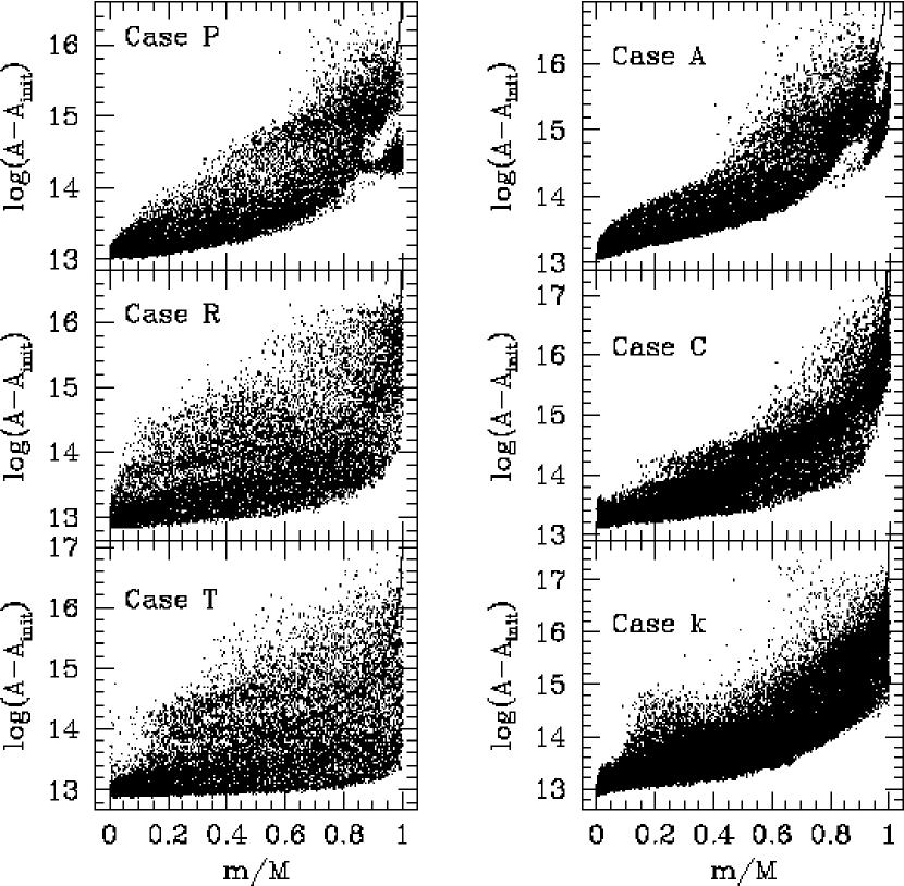
Figure 4: Change in the entropic variable $A$ plotted against the initial enclosed mass fraction $m/M$ for collisions involving identical parent stars. Each point represents an individual SPH particle, and the solid curve gives the typical increase in $A$ predicted by equation (2). Logarithms are base 10 and units are cgs.

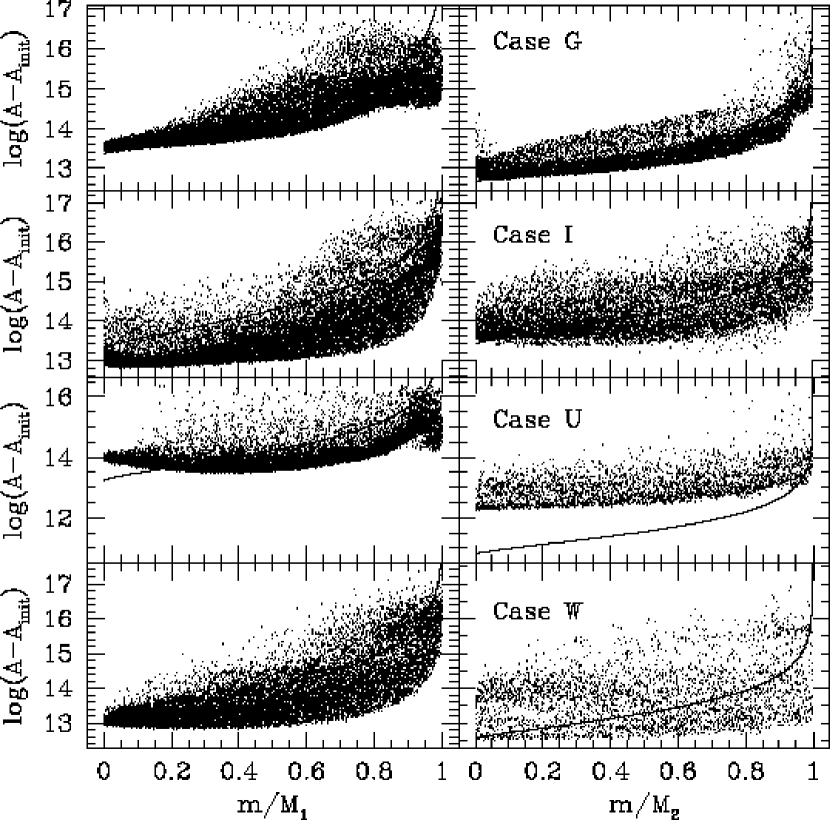
Figure 5: Change in the entropic variable $A$ plotted against the initial enclosed mass fraction $m/M$ for collisions involving parent stars of unequal mass. For each collision scenario, the left and right column displays data for the larger and the smaller star, respectively. Each point represents an individual SPH particle, and the solid curve gives the typical increase in $A$ predicted by equation (2). Logarithms are base 10 and units are cgs.

Clearly, expressions for describing shock heating such as equations (2), (3) and (4) are rather crude approximations that lump together complicated effects from the various stages of the fluid dynamics. However, these expressions do work quite well for parent stars of similar mass. To demonstrate this point, Figure 4 compares the shock heating of this method against the heating experienced by the individual SPH particles in six different collisions of identical parent stars, while Figure 5 presents similar data for four collisions between unequal mass parents. The agreement between prediction and simulation is excellent for mass ratios $M_{1}/M_{2}$ from 1 to approximately 2, regardless of the periastron separation $r_{p}$. Even for a mass ratio as large as 5, the prescription continues to work well, at least for intermediate values of the periastron separation $r_{p}$ (see Case W in Fig. 5). For head-on collisions with large mass ratios, the predicted shock heating is an underestimate in the smaller star and in the center of the larger star (see Case U in Fig. 5). It is worth noting that in collisions between two MS stars, a remnant must be relatively far past the turnoff on a CMD if it is to be identified as a blue straggler. It is therefore unlikely that collisions involving parent stars with a mass ratio more than 5 will produce a true blue straggler, simply because the remnant mass could not be considerably more than the turnoff mass.

The SPH data in Figures 4 and 5 clearly shows that fluid from the same initial enclosed mass fraction $m/M$ can be shock heated different amounts. This effect can be easily understood since, for example, fluid on the impact side of a star will be heated more than fluid with the same $m/M$ on the back side. The treatment of mixing in §2.3 does allow us to model this spread in shock heating, by redistributing fluid to positions with slightly higher or lower final $A$ values than what is given by equation (2). The extent of the redistribution is set by the smoothing parameter $\alpha$ [see eq. (10)], taken to be constant over each parent star. Larger values of $\alpha$ correspond to a smaller width of mass fractions over which the fluid is distributed. The parameter $\alpha=248$, for example, for the parents in Case a, while for Case g, $\alpha_{1}=229$ for the $0.8M_{\odot}$ parent and $\alpha_{2}=143$ for the $0.4M_{\odot}$ parent. This approach does well at mimicking the overall effects of the spread in shock heating. However, mixing of fluid is somewhat overestimated in the core and underestimated in the outer layers, affecting predictions for the central concentration of helium (see §3.1.3) and for the surface concentration of trace elements such as lithium (see §3.1.2). Future treatments could perhaps improve results by implementing a position dependent $\alpha$.

Note that our shock heating prescription does necessarily imply the desirable qualitative features that are discussed in §2.2 and evident in the SPH data of Figures 4 and 5: (1) fluid with large initial pressure $P_{init}$ (the fluid shielded by the outer layers of the star) is generally shock heated less, (2) $b_{2}(0)\leq b_{1}(0)$, so that a less massive star is shock heated less in head-on collisions, (3) $b_{1}(r_{p})$ decreases with $r_{p}$ while $b_{2}(r_{p})$ increases with $r_{p}$, so that for sufficiently large $r_{p}$ we have $b_{2}(r_{p})>b_{1}(r_{p})$ and the less massive star is shock heated more, and (4) $b_{1}(r_{p})=b_{2}(r_{p})$ whenever $M_{1}=M_{2}$, so that identical parent stars always experience the same level of shock heating.

3.1.2 Mass Loss

Although mass loss is very small in a parabolic collision, it is nevertheless important to understand well if one is interested in tracking trace elements that may only be found in outermost layers of the parent stars. The method of §2.1 yields remnant masses that are seldom more than $\sim 0.01M_{\odot}$ different than what is given by a hydrodynamic simulation (see the last two columns of Table 2); this is clearly a significant improvement over neglecting mass loss completely, which sometimes can overestimate the remnant mass by more than $\sim 0.1M_{\odot}$. Table 2 also lists the fraction $f_{2}$ of the ejecta that originated in star 2 for each collision scenario, both as calculated from our simple method and as calculated from an SPH simulation. Our simple method allows for the determination of $f_{2}$ simply by requiring that the outermost fluid retained from each of the parent stars has the same post-shock entropy. Again, the agreement between prediction and simulation is excellent, especially for cases with mass ratios $M_{1}/M_{2}\lesssim 2$.

The mass loss and merging procedures implemented in this paper allow one to identify not only how much of the ejecta originated in each parent star, but also the original location of the fluid within each parent. The expression $g_{ik}\Delta m_{i}\Delta m_{k}/(\sum_{j}g_{ji}\Delta m_{j})$ gives the amount of mass in shell $i$ that is transported to shell $k$ [cf. eq. (8)]. Therefore the fraction of the mass from shell $i$ that ultimately becomes ejecta is given by

$$f_{ejecta,i}={\sum_{k>k_{max}}g_{ik}\Delta m_{k}\over\sum_{j}g_{ji}\Delta m_{j}},$$ (16)

where $k_{max}$ corresponds to the shell with the highest entropy fluid still gravitationally bound to the remnant. In equation (16), the sum over shells $k$ includes only those shells with larger post-shock entropies than this maximum, that is, only those shells associated with ejecta. Figure 6 displays the $f_{ejecta}$ curves for the parent stars in a variety of different collision scenarios, both as determined by this method and as determined by an SPH calculation.

Lithium is a particularly interesting element to follow during a collision. Lithium is burned during stellar evolution except at low temperatures, and therefore can be used as an indicator of mixing. If a star has a deep enough surface convective layer, there will be essentially no lithium, because the convection mixes any lithium from the outer layers into the hot interior where it is burned. A small amount of lithium does exist in the outer few percent of, for example, a $0.8M_{\odot}$ turnoff star (see Fig. 2) and would consequently become part of the ejecta during a collision, resulting in a remnant with very little lithium.

3.1.3 Structure and Composition

Thermodynamic (Fig. 7) and chemical composition (Figs. 8, 9, 10 and 11) profiles show that our remnant models are quite accurate. In Case g, our remnant displays the kink in the $A$ profile near $m/M=0.1$ (see Fig. 7), inside of which the fluid originates solely from the $0.8M_{\odot}$ star. Our models also reproduce the chemical profiles of the SPH remnant very well: the peak values in the chemical abundances are often accurate to within 20%, and the shapes of these profiles, though sometimes peculiar, are followed closely. Helium distribution is particularly important to model well since it will help determine the MS lifetime of the remnant. As mentioned in §3.1.1, the core of the remnant is usually somewhat overmixed, flattening out the helium profile in that region. Nevertheless, the central value of the fractional helium abundance $Y$ given by our models typically underestimates the SPH result by only about 5%.

Although near the remnant’s surface our method sometimes yields a large fractional error in lithium abundance (see Figs. 8 and 9), this is simply because the overall abundance is so close to zero. For example, the predicted surface fractional Li⁶ abundance of $6.9\times 10^{-10}$ for our Case a remnant is an overestimate, but is nearly 20 times smaller than the surface fractional abundance in the $0.8M_{\odot}$ parent. Except for in the extreme case of grazing collisions (when mass loss is exceedingly small), collisional blue stragglers should be severely depleted in lithium, a prediction that can be tested with appropriate observations [see Shetrone & Sandquist (2000) and Ryan et al. (2001)].

3.1.4 Angular Momentum Distribution

Our previous hydrodynamic simulations involving polytropic stars (Lombardi et al., 1996) implemented the classical form of the artificial viscosity (AV), which introduces a significant amount of spurious shear in our differentially rotating remnants. The effects of shear are discussed in §4.2 of Lombardi et al. (1996) and studied in detail in Lombardi et al. (1999). Shear tends to weaken differential rotation, transporting angular momentum outward. This angular momentum transport acts on the viscous timescale, which is comparable to the total time of a typical simulation in our collisions between polytropic stars. We therefore avoid comparisons involving the angular momentum profiles of remnants from our polytropic SPH calculations.

Our collisions between realistically modeled stars implemented the Balsara AV (Balsara, 1995), with a viscous timescale that is significantly larger. In particular, Lombardi et al. (1999) show that the viscous timescale scales approximately with $N_{N}^{1/2}$ for the classical AV (where $N_{N}$ is the neighbor number) and $N_{N}$ for Balsara AV. Since we used $N_{N}=64$ in our polytropic simulations and $N_{N}=100$ in our realistic simulations, the viscous timescale is larger in our collisions involving realistic parent stars by a factor of approximately $100/64^{1/2}\sim 10$. Consequently, in our SPH calculations done with the Balsara AV, only a relatively small amount of specific angular momentum is spuriously transported out from the core.

Specific angular momentum profiles, averaged over surfaces of constant density, are compared in Figure 12 for the three realistically modeled cases with rotating remnants: Cases e, f and k. We find excellent agreement between our simple models and their corresponding SPH counterparts. Our procedure for determining the angular momentum distribution, as described in §2.4, yields values of $k_{1}$, $k_{2}$ and $k_{3}$ of, respectively, 0.161, 0.427 and $3.16\times 10^{16}$ cm²/s for Case e, of 0.023, 0.570 and $5.93\times 10^{15}$ cm²/s for Case f, and of 0.146, 0.415 and $4.56\times 10^{16}$ cm²/s for Case k. Note that the hump in the SPH $j$ profile in the outer few percent of the remnant results from the need to terminate the simulation before all of the gravitationally bound fluid has fallen back to the merger remnant: this artifact is gradually diminishing during the final stages of the SPH calculation.

3.2 Stellar Evolution of Remnant Models

A rigorous test of the validity of the simple models, which we have performed using YREC, is to compare their subsequent stellar evolution against that of SPH-generated models. YREC evolves a star through a sequence of models of increasing age, solving the stellar evolution equations for interior profiles such as chemical composition, pressure, temperature, density and luminosity. All relevant nuclear reactions (including pp-chains, the CNO cycle, triple-$\alpha$ reactions and light element reactions) are treated. Recent opacity tables are used (ensuring that the remnant’s position in a CMD can be accurately determined) and mixing mechanisms are incorporated. For blue stragglers, the various mixing processes can potentially carry fresh hydrogen fuel into the stellar core and thereby extend the MS lifetime of the remnant. Furthermore, any helium mixed into the outer layers affects the opacity and hence the remnant’s position in a CMD. The free parameters in YREC (e.g., the mixing length) are set by calibrating a solar mass and solar metallicity model to the Sun.

Using the method described in Sills et al. (1997), we used two of our simple models (Cases a and g) as starting models in YREC and evolved the collision products from the end of the collision to the giant branch. Figure 13 shows the evolutionary tracks for these simple models (solid lines) and the SPH-generated models (dotted lines). The tracks of the SPH-generated models are discussed in Sills & Lombardi (1997).

The agreement between the two sets of models is very good. Although there are some differences on the ’pre-MS’ portion of the tracks, this stage only lasts for approximately a Kelvin-Helmholtz timescale, a very small fraction of the total lifetime of the cluster. Indeed, for Case a, the SPH and simple models reach the MS after 0.4 Myr and 0.8 Myr, respectively, and the corresponding contraction times for the Case g models are only 4 Myr and 2 Myr. Since the stars contract to the MS so quickly, the exact pre-MS track may not be directly important for generating synthetic CMDs. Nevertheless a reasonable model of a pre-MS star can be of interest: the radius of a newly born remnant, and hence its collisional cross-section in a multi-star interaction, is strongly dependent on how the fluid has been shocked, and furthermore the surface abundances are strongly dependent on how it has been mixed.

Once the collision product reaches the MS, the two methods show very good agreement, and the subgiant and giant branch evolution of these stars is virtually identical. The MS lifetimes for the two different methods agree reasonably well. For Case g, the SPH results give a lifetime of 850 Myr, while the simple models give 650 Myr. For Case a, the SPH results give a lifetime of 80 Myr, compared to 180 Myr from the simple models. It should be noted that the Case a remnant has central helium abundance near 100%, accounting for its short MS lifetime. For such remnants, even a slight inaccuracy in the core’s helium profile has a large relative effect on how long the star remains on the MS. While the MS lifetime resulting from our method can be off by more than a factor of two for remnants with intact helium cores, the lifetime of such remnants is nevertheless a very small fraction of the lifetime of globular clusters, and therefore the simple models can still be useful for incorporating stellar collisions into dynamical models of globular cluster evolution.

4 Concluding Remarks

An important question in the study of globular clusters is what are the necessary features of stellar collisions that must be modeled in order to synthesize reliable theoretical CMDs. While detailed studies of the tracks and evolutionary timescales of rapidly rotating collision remnants will be necessary to answer this question fully, we do feel that the features modeled in this paper (mass loss, shock heating, hydrodynamic mixing, angular momentum distribution) are all essential components to consider. Our treatment of ejecta allows for an accurate estimate of the total mass of the remnant, upon which the subsequent stellar evolution and MS lifetime depend sensitively. Furthermore, shock heating during a collision not only influences the structure of the remnant, but also helps determine if convective regions can develop during the future evolution: the entropy gradients implied by SPH results and by the shock heating method of this paper tend to stabilize a contracting pre-MS star against convection. Previous stellar evolution studies of remnants have found that the tracks are sensitive to the assumptions made about how the fluid is mixed during a merger (Bailyn & Pinsonneault, 1995; Sills & Bailyn, 1999); our simple fluid mixing algorithms give a compromise between previously used approximations that tend to bracket the actual amount of mixing during a collision. Finally, although the treatment of rotation in stellar evolution is a challenging problem, it is clear that rotational support and induced mixing must be considered as they have profound consequences on stellar evolution (Sills, Pinsonneault, & Terndrup, 2000; Sills et al., 2001); the form for the angular momentum distribution presented in this paper provides a simple means of generating very reasonable initial profiles for future studies of collisional remnants.

The algorithms we have developed are implemented in a publicly available FORTRAN software package named “Make Me A Star.” For the forseeable future, this package can be downloaded from http://vassun.vassar.edu/$\sim$lombardi/mmas/. Researchers should be aware of the limitations of this method in terms of the structure, rotational properties and evolutionary timescales of the models created, as outlined in this paper. This software does produce accurate models for a variety of collision scenarios, and we hope that it will be used in combination with realistic dynamical simulations of star clusters that must take into account stellar collisions.

Figure 1: Thermodynamic profiles of $A(=P/\rho^{5/3})$, pressure $P$, and density $\rho$ as a function of enclosed mass $m$. Our three realistically modeled parent stars are displayed in the left column, and the four polytropic models are displayed on the right. The dotted, short-dashed, long-dashed and solid curves refer to $0.8M_{\odot}$, $0.6M_{\odot}$, $0.4M_{\odot}$ and $0.16M_{\odot}$ parent stars, respectively. Logarithms are base 10 and units are cgs.

Figure 2: Fractional chemical abundance (by mass) as a function of enclosed mass $m$ for various chemical elements in our three realistically modelled parent stars. Line types are as in Fig. 1.

Figure 3: The change in entropic variable $A$ as a function of initial pressure $P_{init}$ on a log plot for the SPH remnant of Case e and Case g (see Table 2 for data describing these cases). Pentagons refer to fluid from parent star 1 that has reached dynamical equilibrium by the end of the simulation and that has been binned by enclosed mass fraction; triangles refer to the corresponding fluid from star 2. Logarithms are base 10 and units are cgs.

Figure 6: Local fraction of mass that is ejected by the collision, as a function of the initial enclosed mass $m$ inside each parent star. The dotted curves represent the results of a 3D SPH simulation, while the dashed curves represent the method of this paper. For Cases a, k and A, only a single curve is necessary for each line type, since the parent stars are identical and experience the same mass loss distribution.

Figure 7: Thermodynamic profiles of $A$, pressure $P$, and density $\rho$ as a function of enclosed mass fraction $m/M_{r}$ for the remnants of Cases a and g, where $M_{r}$ is the total bound mass of the remnant. The dotted line refers to the remnant resulting from a 3D SPH simulation, and the dashed line refers to the remnant generated by the method of this paper. Logarithms are base 10 and units are cgs.

Figure 8: Fractional chemical abundance (by mass) as a function of enclosed mass fraction $m/M_{r}$ for the Case a remnant. Line types are as in Fig. 7.

Figure 9: Fractional chemical abundance (by mass) as a function of enclosed mass fraction $m/M_{r}$ for the Case g remnant. Line types are as in Fig. 7.

Figure 10: Fractional chemical abundance (by mass) as a function of enclosed mass fraction $m/M_{r}$ for the Case e remnant. Line types are as in Fig. 7.

Figure 11: Fractional chemical abundance (by mass) as a function of enclosed mass fraction $m/M_{r}$ for the Case k remnant. Line types are as in Fig. 7.

Figure 12: SPH specific angular momentum profiles (dotted curves) compared with the approximate profiles (long dashed curves) generated from equation (15). Logarithms are base 10 and units are cgs.

Figure 13: Evolutionary tracks for Case a and Case g. The solid lines correspond to the tracks of the simple models described in this paper, while the dotted lines show tracks for models generated directly from the output of SPH calculations. The symbols mark identifiable evolutionary phases in the evolution of the collision products: diamonds show the position of the star immediately following the collision. Circles mark the “zero age” MS, squares mark the MS turnoff, and triangles show the base of the giant branch.

Table 1: Parent Star Characteristics

Structure type	$M[M_{\odot}]$	$R[R_{\odot}]$	$R_{0.5}[R_{\odot}]$	$R_{0.86}[R_{\odot}]$
$n=3$ polytrope	0.8	0.955	0.270	0.443
Composite polytrope	0.6	0.535	0.253	0.382
$n=1.5$ polytrope	0.4	0.353	0.184	0.261
$n=1.5$ polytrope	0.16	0.153	0.080	0.113
YREC	0.8	0.955	0.198	0.395
YREC	0.6	0.517	0.203	0.332
YREC	0.4	0.357	0.182	0.272

Table 2: Mass loss

Case	${M_{1}\over M_{\odot}}$	${M_{2}\over M_{\odot}}$	${r_{p}\over R_{1}+R_{2}}$	$f_{2,SPH}$	$f_{2}$	$f_{L,SPH}$	$f_{L}$	${M_{SPH}\over M_{\odot}}$	${M_{r}\over M_{\odot}}$
A	0.8	0.8	0.00	0.50	0.50	0.064	0.064	1.50	1.497
B	0.8	0.8	0.25	0.51	0.50	0.023	0.025	1.56	1.560
C	0.8	0.8	0.50	0.50	0.50	0.012	0.015	1.58	1.577
D	0.8	0.6	0.00	0.24	0.24	0.057	0.061	1.32	1.315
E	0.8	0.6	0.25	0.19	0.26	0.024	0.027	1.37	1.363
F	0.8	0.6	0.50	0.26	0.30	0.008	0.017	1.39	1.376
G	0.8	0.4	0.00	0.049	0.042	0.056	0.054	1.13	1.135
H	0.8	0.4	0.25	0.059	0.065	0.028	0.024	1.17	1.172
I	0.8	0.4	0.50	0.11	0.12	0.008	0.015	1.19	1.182
J	0.6	0.6	0.00	0.50	0.50	0.049	0.059	1.14	1.129
K	0.6	0.6	0.25	0.50	0.50	0.028	0.030	1.17	1.164
L	0.6	0.6	0.50	0.51	0.50	0.022	0.020	1.17	1.175
M	0.6	0.4	0.00	0.11	0.13	0.054	0.055	0.95	0.945
N	0.6	0.4	0.25	0.14	0.18	0.029	0.029	0.97	0.971
O	0.6	0.4	0.50	0.16	0.26	0.010	0.020	0.99	0.980
P	0.4	0.4	0.00	0.50	0.50	0.037	0.056	0.77	0.756
Q	0.4	0.4	0.25	0.51	0.50	0.029	0.030	0.78	0.776
R	0.4	0.4	0.50	0.54	0.50	0.010	0.020	0.79	0.784
S	0.4	0.4	0.75	0.47	0.50	0.008	0.015	0.79	0.788
T	0.4	0.4	0.95	0.51	0.50	0.011	0.013	0.79	0.790
U	0.8	0.16	0.00	0.015	0.001	0.027	0.035	0.93	0.927
V	0.8	0.16	0.25	0.016	0.003	0.025	0.014	0.94	0.946
W	0.8	0.16	0.50	0.024	0.014	0.021	0.009	0.94	0.951
a	0.8	0.8	0.00	0.50	0.50	0.079	0.078	1.47	1.475
e	0.8	0.6	0.25	0.19	0.20	0.029	0.026	1.36	1.363
f	0.8	0.6	0.50	0.21	0.21	0.014	0.016	1.38	1.377
g	0.8	0.4	0.00	0.098	0.039	0.062	0.061	1.13	1.127
k	0.6	0.6	0.25	0.50	0.50	0.032	0.030	1.16	1.164

Table 3: Total Energy

Case	$E_{tot}$	$E_{r,SPH}$	$E_{r}$
	[$10^{48}$g cm2/s2]	[$10^{48}$g cm2/s2]	[$10^{48}$g cm2/s2]
A	-3.81	-4.5	-4.43
D	-3.09	-3.6	-3.56
G	-2.64	-3.1	-3.00
J	-2.37	-2.6	-2.72
M	-1.92	-2.2	-2.19
P	-1.47	-1.6	-1.68
U	-2.18	-2.3	-2.37
a	-5.23	-6.3	-6.25
g	-3.35	-3.9	-3.86

Table 4: Total Angular Momentum

Case	$J_{tot}$	$J_{r,SPH}$	$J_{r}$
	[$10^{51}$g cm2/s]	[$10^{51}$g cm2/s]	[$10^{51}$g cm2/s]
B	2.99	2.84	2.84
C	4.23	4.13	4.10
E	2.12	2.04	2.00
F	2.99	2.93	2.89
H	1.43	1.34	1.36
I	2.02	1.97	1.96
N	0.97	0.91	0.91
O	1.37	1.33	1.31
Q	0.64	0.61	0.60
R	0.91	0.90	0.87
S	1.11	1.10	1.08
T	1.25	1.21	1.22
V	0.59	0.54	0.57
W	0.83	0.75	0.82
e	2.10	1.99	1.99
f	2.97	2.85	2.87
k	1.43	1.36	1.34

References

- Bacon et al. (1996) Bacon, D., Sigurdsson, S., & Davies, M. B. 1996, MNRAS, 281, 830
- Balsara (1995) Balsara, D. 1995, J. Comput. Phys., 121, 357
- Bailyn (1995) Bailyn, C. D. 1995, Ann. Rev. Ast. Astrop., 33, 133
- Bailyn & Pinsonneault (1995) Bailyn, C. D. & Pinsonneault, M. H. 1995, ApJ, 439, 705
- Davies & Benz (1995) Davies, M. B., & Benz, W. 1995, MNRAS, 276, 876
- Endal & Sofia (1976) Endal, A. S., & Sofia, S. 1976, ApJ, 210, 184
- Gilliland et al. (1998) Gilliland, R. L. 1998, ApJ, 507, 818
- Hills & Day (1976) Hills, J. G., & Day, C. A. 1976, Ap. Letters, 17, 87
- Hut et al. (1992) Hut, P., McMillan, S., Goodman, J., Mateo, M., Phinney, E. S., Pryor, C., Richer, H. B., Verbunt, F. & Weinberg, M. 1992, PASP, 104, 981
- Lai, Rasio & Shapiro (1994) Lai, D. Rasio, F. A. & Shapiro, S. L. 1994, ApJ, 423, 344.
- Leonard (1989) Leonard, P. J. T. 1989, AJ, 98, 217
- Leonard & Fahlman (1991) Leonard, P. J. T., & Fahlman, G. G. 1991, AJ, 102, 994
- Livio (1993) Livio, M. 1993, in Blue Stragglers, ASP Conf. Ser. 53, ed. R. A. Saffer (San Francisco: ASP)
- Lombardi et al. (1996) Lombardi, J. C., Rasio, F. A., & Shapiro, S. L. 1996, ApJ, 468, 797
- Lombardi et al. (1999) Lombardi, J. C., Sills, A., Rasio, F. A., & Shapiro, S. L. 1999, J. Comp. Phys., 152, 687
- Monaghan (1992) Monaghan, J. J. 1992, ARA&A, 30, 543
- Rasio & Lombardi (1999) Rasio, F. A., & Lombardi, J. C. 1999, J. Comp. App. Math., 109, 213
- Rasio, Fregeau & Joshi (2001) Rasio, F. A., Fregeau, J. M., & Joshi, K. J. 2001, to appear in The Influence of Binaries on Stellar Population Studies, ed. D. Vanbeveren (Dordrecht: Kluwer). [astro-ph/0103001]
- Ryan et al. (2001) Ryan, S., Beers, T., Kajino, T. & Rosolankova, K. 2001, ApJ, 547, 231
- Sandquist et al. (1997) Sandquist, E. L., Bolte, M. & Hernquist, L. 1997, ApJ, 477, 335
- Sepinsky et al. (2000) Sepinsky, J. F., Saffer, R. A., Pilman, C. S., DeMarchi,G., & Paresce, F. 2000, AAS Meeting 196, #41.06
- Shara et al. (1997) Shara, M. M., Saffer, R. A., & Livio, N. 1997, ApJ, 489, L59
- Shetrone & Sandquist (2000) Shetrone, M. D., & Sandquist, E. L. 2000, AJ, 120, 1913
- Sigurdsson et al. (1994) Sigurdsson, S., Davies, M. B., & Bolte, M. 1994, ApJ, 431, L115
- Sigurdsson & Phinney (1995) Sigurdsson, S., & Phinney, E. S. 1995, ApJS, 99, 609
- Sills & Bailyn (1999) Sills, A., & Bailyn, C. D. 1999, ApJ, 513, 428
- Sills & Lombardi (1997) Sills, A. & Lombardi, J. C. 1997, ApJ, 484, L51
- Sills et al. (1997) Sills, A., Lombardi, J. C., Jr., Demarque, P. D., Bailyn, C. D., Rasio, F. A., & Shapiro, S. L. 1997, ApJ, 487, 290
- Sills et al. (2000) Sills, A., Bailyn, C. D., Edmonds, P. D., & Gilliland, R. L. 2000, ApJ, 535, 298
- Sills et al. (2001) Sills, A., Faber, J. A., Lombardi, J. C., Rasio, F. A., & Warren, A. R. 2001, ApJ, 548, 323
- Sills, Pinsonneault, & Terndrup (2000) Sills, A., Pinsonneault, M. H., & Terndrup, D. M. 2000, ApJ, 534, 335
- Stryker (1993) Stryker, L. L. 1993, PASP, 105, 1081
- Tassoul (1978) Tassoul, J. 1978, Theory of Rotating Stars (Princeton: Princeton Univ. Press)
- Tassoul (2000) Tassoul, J. 2000, Stellar Rotation (Cambridge: Cambridge Univ. Press)